Simulation of the Single- and Double-Slit Experiments with Quantum Walkers

Abstract

We employ the broken-link model to create a barrier with slits in a two-dimensional lattice. The diffraction and interference patterns of the probability distribution of quantum walkers passing through the slits are analyzed. Simulations were performed using the main types of coins, and display diffraction and interference patterns that depend on the choice of coins.

I Introduction

The main models of quantum walks, known as discrete-time and continuous-time, were introduced by Aharanov, Davidovich, and Zagury Aharonov and Farhi and Gutmann Farhi , respectively. Both of those models present radically new features when compared to the classical random walk, one of the most remarkable is that quantum walks spread in a ballistic way, in contrast with the diffusive behavior of classical random walkers. This property motivated many studies pursuing to introduce quantum algorithms much faster than their classical counterparts Farhi ; Shenvi ; Ambainis .

Many papers in the recent literature address the theory of one-dimensional quantum walks in order to understand both its physical properties and possible applications Aharonov ; Nayak . However, in the general case, there are some properties that appear only in two or higher dimensions. In our previous work on decoherence in two-dimensional quantum walks Oliveira , we have shown that, when increasing the decoherence rate in an appropriate way, there is a transition from a decoherent two-dimensional to a coherent one-dimensional quantum walk. To obtain this result, we have employed the broken-link decoherence method introduced by Romanelli et al. for the one-dimensional case Romanelli . In order to extend the broken-link method to higher dimensional walks, in Oliveira we have generalized the evolution equation to generic broken-link topologies and lattices of any dimension.

As shown in the present work, that generalized evolution equation can also be used to study quantum walks with rather arbitrary boundary conditions. The freedom to choose the boundary conditions allows to study random walks on a large variety of topologies. In order to illustrate the method, we study here the behavior of quantum walkers passing through one and two slits. The standard double-slit experiment using light waves (Young’s experiment) proved conclusively the wave nature of light Born and has notedly been employed by Feynman to illustrate the differences between the classical and quantum worlds Feynman . We found interesting to ascertain, in the case of quantum walkers, which as noted possess ballistic properties, but are not characterized by a single wavelength, whether they would display diffraction and interference patterns, or would behave more as classical particles.

Our analysis is based on the simulation of different kinds of quantum walkers moving on a region of the two-dimensional lattice illustrated on Fig. 1. Notice that, as in Ref. Oliveira , the lattice links are parallel to the main or secondary diagonals of the grid. The walker starts at one point on the lattice, indicated by an open circle, and moves due to the successive application of the (unitary) evolution operator, as is usual in the theory of quantum walk. At some point not very close to the origin of the evolution, there is a barrier perpendicular to the horizontal axis with either one or two slits. The barrier consists of a succession of sites with broken links between them, while the slits correspond to sites with working links. At some distance from the barrier there is a screen, also perpendicular to the horizontal axis, which accumulates the value of the probability as the walker passes. The general setup is similar to the standard Young’s double-slit interference experiment.

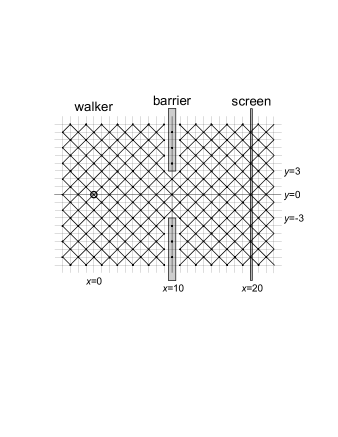
Figure 1: General setup of the simulation at $t=0$. The walker is in the node $x=y=0$. At $x=10$ there is a barrier with one slit of 3 units wide. The barrier is made of a line of sites with the links broken. At $x=20$ there is a screen.

Nowadays, double-slit experiments are performed such that only one particle passes at a time, proving that quantum mechanics describes correctly the one-particle interference pattern. The same strategy is used in the present simulations. We analyze the interference pattern in the screen by considering the equation for the evolution of a single quantum walker. From the analysis of the probability distribution we predict what would happen in actual experiments.

We have organized the paper as follows. In Sec. II we review the equations that govern the evolution of a quantum walker in 2-D lattices with broken links. The diffraction and interference patterns of walkers passing through one slit is analyzed Sec. III and the double-slit case in Sec. IV. A general discussion with conclusions and suggestions for further studies is presented in the last section of this work.

II Quantum Walks with Boundary Conditions

We review here the main elements needed to study the evolution of a quantum walker moving on a 2-D lattice with broken links. Full details of this treatment may be found in Ref. Oliveira .

A coined quantum walk on an infinite two-dimensional lattice takes place on a Hilbert space $\mathcal{H}_{4}\otimes\mathcal{H}_{\infty}$, where $\mathcal{H}_{4}$ is the coin space and $\mathcal{H}_{\infty}$ is the lattice space. The coin consists of two qubits with basis $\{{\left|j,k\right\rangle},j,k\in\{0,1\}\}$. As mentioned above, we consider that the links are along either the main or the secondary diagonals of the lattice. Thus, the basis for $\mathcal{H}_{\infty}$ is $\{{\left|m,n\right\rangle},m,n\,{\rm integers}\}$ such that $m+n$ is even.

The generic state of the quantum walker is given by the wavefunction

$${\left|\psi(t)\right\rangle}=\sum_{j,k=0}^{1}\sum_{m,n=-\infty}^{\infty}A_{j,k;\,m,n}(t){\left|{j,k}\right\rangle}{\left|m,n\right\rangle}.$$ (1)

The evolution operator for a single step of the walk is $U=S\circ(C\otimes I)$, where

$$C{\left|j^{\prime},k^{\prime}\right\rangle}=\sum_{j,k=0}^{1}C_{j,k;\,j^{\prime},k^{\prime}}{\left|j,k\right\rangle}$$ (2)

is the coin operator, $I$ is the identity matrix, and $S$ is the shift operator given by

$$S{\left|j^{\prime},k^{\prime}\right\rangle}{\left|m,n\right\rangle}=\sum_{j,k=0}^{1} \left[1-\delta_{j,j^{\prime}}-(-1)^{j^{\prime}}\right.\left.{\mathcal{L}_{1}}(1-j,1-k;\,m+(-1)^{j}\delta_{j,j^{\prime}},n+(-1)^{k}\delta_{k,k^{\prime}})\right]\times$$

$$\left[1-\delta_{k,k^{\prime}}-(-1)^{k^{\prime}}\right.\left.{\mathcal{L}_{2}}(1-j,1-k;\,m+(-1)^{j}\delta_{j,j^{\prime}},n+(-1)^{k}\delta_{k,k^{\prime}})\right]\times$$

$$|j,k\rangle|m+(-1)^{j}\delta_{j,j^{\prime}},n+(-1)^{k}\delta_{k,k^{\prime}}\rangle,$$

where $\mathcal{L}_{1}$ and $\mathcal{L}_{2}$ are two auxiliary functions required to specify the broken links, one for each direction. These functions are described by

$$\mathcal{L}_{1}(j,k;\,m,n)=\begin{cases}(-1)^{j},&\mbox{if {\rm link} to site $m+(-1)^{j}$,}\mbox{$n+(-1)^{k}$ is closed,}\\ 0,&\mbox{if {\rm the link} is open,}\end{cases}$$ (4)

and

$$\mathcal{L}_{2}(j,k;\,m,n)=\begin{cases}(-1)^{k},&\mbox{if {\rm link} to site $m+(-1)^{j}$,}\mbox{$n+(-1)^{k}$ is closed,}\\ 0,&\mbox{if {\rm the link} is open,}\end{cases}$$ (5)

where $j,k\in\{0,1\}$.

When the links are unbroken, the walker moves along the main diagonal, if the value of the coin is ${\left|0,0\right\rangle}$ or ${\left|1,1\right\rangle}$, or along the secondary diagonal if the value of the coin is ${\left|0,1\right\rangle}$ or ${\left|1,0\right\rangle}$. If some links are broken, the walker moves, or stands still, in such a way that the probability flux is conserved and the evolution is unitary. This is assured by the evolution equations Oliveira :

$$A_{1-j,1-k;\,m,n}(t+1)=\sum_{{j^{\prime},\,k^{\prime}}=0}^{1}C_{j+\mathcal{L}_{1}\left(j,k;\,m,n\right),k+\mathcal{L}_{2}\left(j,k;\,m,n\right);\,{j^{\prime}},{k^{\prime}}}\,A_{{j^{\prime}},{k^{\prime}};m+\mathcal{L}_{1}\left(j,k;\,m,n\right),n+\mathcal{L}_{2}\left(j,k;\,m,n\right)}(t).$$ (6)

In the next sections, we analyze the diffraction and interference patterns produced by quantum walkers passing through one and two slits. We use the Hadamard, Fourier, and Grover coins in the simulations. The initial conditions are the same used in Ref. Oliveira , except for the Hadamard walker, which is

$${\left|\psi(0)\right\rangle}=\frac{1}{2}({\left|0\right\rangle}+i{\left|1\right\rangle})({\left|0\right\rangle}+i{\left|1\right\rangle}){\left|0,0\right\rangle}.$$

The analysis is based on the probability distribution, which is given by

$$P_{m,n}(t)=\sum_{j,k=0}^{1}{\left|A_{j,k;\,m,n}(t)\right|}^{2}.$$ (7)

As in the one-dimensional case, there is a parity pattern in the probability distribution in the 2-dimensional case, when there are no broken links. If the probability at one site of the lattice is not zero, the probability at the neighboring sites should be zero. When there are broken links, as in the slitted barrier, the reflections on the incidence side will destroy this parity pattern. However, the wave that passes through the slit(s) conserves the parity pattern. To clarify the description we shall plot only the non-zero probabilities.

III The single-slit case

The simulation of a quantum walker passing through one slit displays many interesting physical properties. Some of those are similar to the ones that appear in the standard diffraction of waves passing through one slit. In Fig. 2, one can see diffraction patterns after the Hadamard walker has passed through one slit five units wide . Around $x=56$ there is a dominant wavefront, which has a smooth central peak surrounded by two secondary small peaks. The central peak is produced by constructive interference and has a nature different from the usual pattern of the Hadamard walker, which has the highest peaks at the corners, not at the center of the side Oliveira . The peaks at $x=-56$ are similar to those appearing for in the free Hadamard walker, as it could be expected. The peaks between $x=-20$ and $x=20$ are produced by the walkers reflected at the barrier. As discussed below, besides these similarities in the diffraction and interference patterns of quantum walkers and the standard single-slit interference experiment, there are also some noticeable differences.

Figure 2: Probability distribution of the Hadamard walker after 80 iterations. The slit has a width of 5 units, and the barrier is placed at $x=20$.

Fig. 3 shows the probability distribution accumulated at the screen ($I$) from $t=0$ until $t=100$ for the Hadamard walker. We use the term accumulated in the following sense: For each value of $y$ at the screen, we add up the values of the probability from $t=0$ until $t=100$. At $t=100$, the dominant contribution of the wave has already passed through the screen. Note that in the previous figure, at $t=80$ the wavefront has just arrived at the screen, which is located at $x=60$. In Fig. 3, each curve corresponds to a slit width (listed at the top). One can clearly see diffraction and interference patterns. For each slit width, there is a central peak produced by constructive interference and one local minimum at each side produced by destructive interference. There are also secondary maxima and minima. We found interesting to obtain these patterns, as it is well known that the quantum walker Fourier spectrum contains many different wavelengths Nayak . The similarities with the standard single-slit diffraction pattern are due to the dominance of particular wavelengths in the quantum walker spectrum, and the differences to the multiplicity of those wavelengths. The value of the intensity of the central peak increases when the width increases until 9, but for larger widths, the central peak decreases, gradually changing the pattern into the usual Hadamard peaks at the extrema without intermediate diffraction effects.

Figure 3: The probability distribution accumulated at the screen of the Hadamard walker. The number of iterations is 100 and the slit widths are 5, 9, and 13. The barrier is placed at $x=20$ and the screen is positioned at $x=60$.

IV The Double-Slit Case

In the Young’s double-slit experiment, the intensity pattern at the screen displays fringes produced by the interference of the waves coming from each slit. The fringes are modulated by the diffraction and interference due to the finite size of the slits. If the slit width is small compared to the wavelength of the light, the fringes are modulated by one large central peak. A similar kind of pattern can be seen in Fig. 4 for the Hadamard walker. We have amplified the probability distribution of the wave that has passed through the slits by a factor of 5. The figure shows diffraction and interference patterns. There are five peaks produced by constructive interference interlaced by four valleys produced by destructive interference. The wavefront is spread, as we have said before, due to the small size of the slits compared to the order of the smallest wavelengths present in the Fourier spectra of the quantum walker. Note that the wavefront is flat and located around $x=70$. In Young’s experiment, the wavefront is a semi-circle. This flatness is a characteristic of the Hadamard walker, produced by quantum interference effects. Simulations with Grover and Fourier coins yield a curved wavefront. Another difference from Young’s experiment is that the wavefront width is limited by the extrema $y=100$ and $y=-100$. Outside this boundary, the wave function is exactly zero.

Figure 4: The probability distribution of the Hadamard walker after 100 iterations after having passed through a barrier positioned at $x=20$ with two slits of width 1 centered at $y=6$ and $y=-6$. The probability distribution of the diffracted wave ($x>20$) is amplified by a factor of 5.

Fig. 5 shows the distribution of probability accumulated at the screen from $t=0$ until $t=100$ for the Hadamard walker in the same settings of Fig. 4. It is possible to see in details the sequence of alternating maxima and minima inside a large envelope. The figure also depicts the probability distributions accumulated at the screen when one slit is closed and the other is open (dotted and dashed lines). Note that if one adds up these curves, the result does not yield the pattern of interference fringes. This result shows the wavelike behavior of the walker. Note that the intensity at the first minimum is close to zero, showing that the waves that come from the slits have high coherence.

Figure 5: The probability distribution accumulated at the screen of the Hadamard walker in the same settings of the previous figure. The screen is positioned at $x=60$. The dashed curve is the probability distribution when the lower slit is closed and upper slit is open. The dotted curve is the inverse case.

Figure 6: The probability distribution accumulated at the screen of the Grover walker after 120 iterations after having passed through two slits at $x=30$ and screen at $x=70$. The positions of the slit centers are $y=6$ and $y=-6$. The slit width is 1.

It is interesting to analyze the physical behaviour for the Grover and Fourier coins. Fig. 6 shows the probability distribution accumulated at the screen of the Grover walker after having passed through two slits. The figure also shows the distributions of probability when one slit is closed and the other is open. Note that these isolated curves do not display interference fringes. They consist of one peak. When both slits are open, the interference pattern is characterized by a sharp central peak surrounded by two smaller peaks, one at each side. Note that the intensity at the minimum points is high. One can understand this fact by analyzing the oscillating pattern (many wavelengths) of the Grover wavefront at the $x$-axis, for example in Ref. Oliveira . The oscillations are smoother along the main diagonal, where one finds a single characteristic wavelength. In fact, by putting the slits on a barrier perpendicular to the main diagonal, one gets minimum points with low intensity similar to the Hadamard walker. On the other hand, in all simulations with the Grover walker we found three peaks, while for the Hadamard walker we have obtained up to 9 peaks. Our simulations show that the Fourier walker behaves in a way similar to the Grover walker.

V Conclusions

We have analyzed the diffraction and interference patterns of the probability distribution of quantum walkers passing through one and two slits. We have used the evolution equation of quantum walkers in two-dimensional lattices with broken links. The barrier with the slits are generated by breaking permanently the appropriate links. The general setup is similar to the one in the Young’s double-slit interference experiment. We have performed simulations using the Hadamard, Grover, and Fourier coins. The initial condition for the position is the lattice center and for the coin is the one with maximum spreading rate.

In all simulations, diffraction and interference patterns were generated at the screen. As expected, there are similarities and differences between the quantum walker diffraction and interference patterns and the Young-experiment patterns. The similarities between these physical phenomenon displays the wavelike behavior of quantum walkers. The differences can be explained by the following facts. (1) It is known that the Fourier spectrum of the one-dimensional Hadamard walker contains a plethora of wavelengths Nayak . The same is possibly true for Grover and Fourier coins. In contrast, in Young’s interference experiment, the photons have a single wavelength. (2) The quantum walker evolution operator is different from the one used for free-moving fotons.

In future works, we are interested to introduce partial measurements to analyze the complementarity relation between the appearance of interference fringes and the knowledge of which slit the walker has passed. This analysis goes in the direction of Brukner and Zeiliger’s work Brukner on the finiteness of information in Young’s experiment. Besides, the possibility of arbitrarily selecting the shape of the region where the quantum walkers propagate, allows to verify the properties of these systems in a variety of relevant configurations, e.g. chaotic billiards or moving walls.

References

- (1) Y. Aharonov, L. Davidovich, and N. Zagury, Phys. Rev. A 48, 1687-1690 (1993).
- (2) E. Farhi and S. Gutmann, Phys. Rev. A 58, 915-928 (1998).
- (3) N. Shenvi, J. Kempe, and K. BirgittaWhaley, Phys. Rev. A 67, 052307 (2003).
- (4) A. Ambainis, Proc. 45th Symp. Found. Comp. Sc., IEEE Computer Society Press, pp. 22-31, New York, 2004.
- (5) A. Nayak and A. Vishwanath, arXiv:quant-ph/0010117 (2000).
- (6) A.C. Oliveira, R. Portugal, and R. Donangelo, Phys. Rev. A 74, 012312 (2006).
- (7) A. Romanelli, R. Siri, G. Abal, A. Auyuanet, and R. Donangelo, Physica A, 347C, 137-152 (20056), also in arXiv:quant-ph/0403192.
- (8) M. Born and E. Wolf, Principles of Optics, Pergamon Press, Oxford, 1980.
- (9) R.P. Feynman, R.B. Leighton, and M. Sands, The Feynman Lectures on Physics, Vol. 3, Addison-Wesley, Boston, 1965.
- (10) Č. Brukner and A. Zeilinger, Phil. Trans. R. Soc. Lond. A 360, 1061 (2002), e-print arXiv:quant-ph/0201026.