The Stellar-Disk Electric (Short) Circuit: Observational Predictions for a YSO Jet Flow

Abstract

We discuss the star-disk electric circuit for a young stellar object (YSO) and calculate the expected torques on the star and the disk. We obtain the same disk magnetic field and star-disk torques as given by standard magnetohydrodynamic (MHD) analysis. We show how a short circuit in the star-disk electric circuit may produce a magnetically-driven jet flow from the inner edge of a disk surrounding a young star.

An unsteady bipolar jet flow is produced that flows perpendicular to the disk plane. Jet speeds of order hundreds of kilometres per second are possible, while the outflow mass loss rate is proportional to the mass accretion rate and is a function of the disk inner radius relative to the disk co-rotation radius.

Keywords Accretion disks $\cdot$ Stellar magnetospheres $\cdot$ Outflows

1 Star-Disk Magnetic Interaction

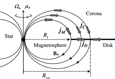
Figure 1: Current flows in the inner section of a star/disk circuit. $j_{D}$ - disk current, $j_{M}$ - field aligned stellar magnetosphere current, $j_{C}$ - field aligned coronal currents $R_{t}$ - inner disk truncation radius, $R_{co}$ - co-rotation radius. If the stellar magnetic field pointed in the opposite direction, to that shown in the figure, then the direction of the current flows would reverse.

Most studies of the electro-magnetic interaction between young stars and their nascent discs undertake their analysis using the standard magnetohydrodynamic (MHD) approximations (Uzdensky 2004). This approach has the advantage of describing the Lorentz force in terms of magnetic fields and allows an analysis that can ignore electric fields and currents. In this paper, we examine the star-disk electric circuit to see if we not only obtain the same answers as standard MHD analysis, but also if we can gain new insight into how accretion disks and bipolar jets may be related in young stellar systems.

It is assumed that a star is rotating with an angular frequency $\Omega_{*}$, it has a dipole magnetic field $B_{*}$, and that the magnetic moment $\mu_{*}$ is aligned with the rotational axis ($\hat{\mbox{\boldmath$\mu$}}_{*}=\hat{\mbox{\boldmath$\Omega$}}_{*}$), which is perpendicular to the plane of the disk (Fig. 1). The direction of $B_{*}$ is such that the $z$ component is negative as it passes through the accretion disk.

The stellar magnetic field truncates the disk at a radial distance $R_{t}$ from the centre of the star, where

$$R_{t}\approx\left(\frac{4\pi}{\mu_{0}}\frac{B_{*}^{2}R_{*}^{6}}{\dot{M}_{a}\sqrt{GM_{*}}}\right)^{2/7}\ =0.067\times$$ (1)

$$\left(\frac{\left(B_{*}(R_{*})/0.1\ {\rm T}\right)^{2}\left(R_{*}/2{\rm R}_{\odot}\right)^{6}}{\left(\dot{M}_{a}/10^{-8}\ {\rm M}_{\odot}\ {\rm year}^{-1}\right)\left(M_{*}/{\rm M}_{\odot}\right)^{1/2}}\right)^{2/7}\ {\rm AU},$$

with $\mu_{0}$ the permeability of free space, $\dot{M}_{a}$ the disk mass accretion rate, $B_{*}(R_{*})$ is the magnetic field strength at the surface of the star, $R_{*}$ is the radius of the star, $M_{*}$ the stellar mass and $G$ the universal gravitational constant.

The co-rotation distance, $R_{co}$, is the radial distance from the star where the angular frequency of the stellar magnetic field ($\approx\Omega_{*}$) equals the Keplerian angular frequency of the disk $\Omega_{K}(r)$:

$$R_{co}=\left(\frac{GM_{*}}{\Omega_{*}^{2}}\right)^{1/3}$$ (2)

$$=0.078\ \left(\left(\frac{M_{*}}{{\rm M}_{\odot}}\right)\left(\frac{P_{*}}{8\ {\rm days}}\right)^{2}\right)^{1/3}\ {\rm AU}\ ,$$

with $P_{*}$ the rotational period of the star. $\Omega_{K}(r)$ is given by the equation

$$\Omega_{K}(r)=\sqrt{\frac{GM_{*}}{r^{3}}}\ .$$ (3)

The relative difference in angular velocity between the disk and the co-rotating stellar magnetic field generates a current within the disk. In Fig. 1, we show a section of the stellar/disk circuit. Here the current density generated within the disk, $j_{D}$, travels along the inner stellar magnetic field lines, $j_{M}$, and then returns to the disk via the outer stellar magnetic field lines in the corona above the disk, $j_{C}$. Only the current flow between $R_{t}$ and $R_{co}$ is shown. The full star-disk circuit is shown in Bardou & Heyvaerts (1996).

2 The Star-Disk Electric Circuit

In Fig. 2, we schematically depict the current flows in and around the inner region of the disk. The electric field in the disk, $\mbox{\boldmath$E_{D}$}(r)$, is given by (Liffman and Bardou 1999)

$$\mbox{\boldmath$E_{D}$}(r)=r\left(\Omega_{K}(r)-\Omega_{*}\right)B_{*z}(r)\hat{\mbox{\boldmath$r$}},$$ (4)

$${\rm with}\ |B_{*z}|(r)\approx B_{*}(R_{*})\left(\frac{R_{*}}{r}\right)^{3}\ ,$$ (5)

where, from Fig. 1, $B_{*z}(r)=-|B_{*z}(r)|$.

For a disk with finite conductivity, $\sigma_{D}$, the induced electric field drives a radial current in the disk with a current density of the form

$$\mbox{\boldmath$j$}_{D}(r)=-\sigma_{D}(r)r\Omega_{K}(r)\left[\left(\frac{r}{R_{co}}\right)^{3/2}-1\right]B_{*z}(r)\ \hat{\mbox{\boldmath$r$}}.$$ (6)

This radial disk current generates a toroidal magnetic field in the disk. The equation for which is (Campbell 1992):

$$B_{\phi}=\mu_{0}\sigma rz(\Omega_{*}-\Omega_{K}(r))B_{z}(r)\ .$$ (7)

Campbell used standard MHD to derive Eqn (7), but the same result is also obtained from the current flow model of Fig. 2 (Liffman & Bardou 1999).

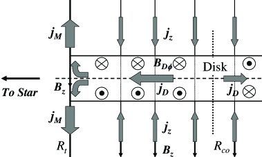
Figure 2: Current flows and magnetic fields near or in the disk. The poloidal field, $B_{z}$, is the section of the stellar magnetosphere that interacts with the disk. The toroidal disk field, $B_{D\phi}$, and the current flows are generated by the relative motion between the disk and $B_{z}$. In this case, $j_{D}$ is the disk current density, $j_{M}$ is the magnetospheric current density that travels between the inner edge of the disk and the star, while $j_{z}$ is the $z$ component of $j_{C}$: the current between the star and the disk.

To compute the field aligned current, $j_{z}$ $i.e.$, the $z$ component of $j_{C}$ that enters the disk (Fig. 2), we apply the steady state form of conservation of electric charge ($\nabla\!\cdot\mbox{\boldmath$j$}=0$), which implies

$$j_{z}=\frac{-1}{\beta\mu_{0}r}\left[\left(\frac{r}{R_{co}}\right)^{3/2}-\frac{5}{2}\right]B_{*z}(r)\ ,$$ (8)

where $\beta$ is a non-dimensional parameter with the definition (Matt and Pudritz 2005)

$$\beta^{-1}=\mu_{0}\sigma_{D}rh\Omega_{K}(r)=2.8\times$$

$$\left(\frac{\sigma_{D}}{10^{-7}\ {\rm Sm^{-1}}}\right)\left(\frac{r}{0.1\ {\rm AU}}\right)\left(\frac{h}{10^{-3}{\rm AU}}\right)\left(\frac{\Omega_{K}}{10^{-5}\ {\rm s}}\right)\ ,$$

with $h$ being the scale height of the disk.

We denote by $I_{M}$ the total current from the top or bottom half of the inner disk ($i.e.$, the inner edge located at the truncation radius, $R_{t}$) that travels along the stellar field lines to the star (the corresponding current density, $j_{M}$ is shown in Fig. 1). the magnitude of $I_{M}$ is given by (using Eqn (6))

$$I_{M}=\frac{2\pi R_{t}}{\mu_{0}\beta}\left|\left(\frac{R_{t}}{R_{co}}\right)^{3/2}-1\right||B_{*z}(R_{t})|\ .$$ (10)

A representative value for the magnitude of $I_{M}$ is given by

$$I_{M} = 8.6\times 10^{12}\left(\frac{0.05\ {\rm AU}}{R_{t}}\right)^{2}\left(\frac{B_{*}(R_{*})}{0.1\ {\rm T}}\right)\times$$ (11)

$$\left(\frac{2.8}{\beta}\right)\left(\frac{R_{*}}{2{\rm R}_{\odot}}\right)^{3}\left|\left(\frac{R_{t}}{R_{co}}\right)^{3/2}-1\right|\ {\rm A}.$$

3 Disk-Star Torque

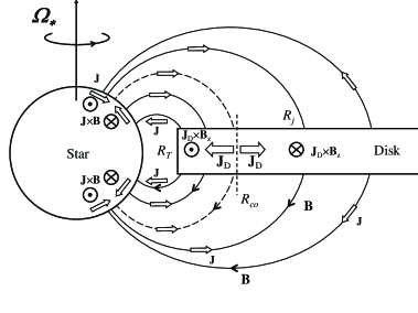
Figure 3: The interaction of an assumed bipolar stellar magnetic field, $B$ and the disk produces current flows, $J$, (denoted by fat arrows) that, in turn, create $\mbox{\boldmath$J$}\times\mbox{\boldmath$B$}$ forces which act upon the star and the disk. For the system shown, the general rotation is anticlockwise when viewed from above. The $\bigodot$ and $\bigotimes$ symbols represent the Lorentz force pointing in the direction towards and away from the observer, respectively.

To determine the torque(s) on the disk, we consider an annulus of the disk, which has a radius of $r$, thickness $\Delta r$ and height $2h$. The volume, $\Delta V$, of the annulus is $4\pi rh\Delta r$ and it feels a torque

$$\Delta\tau=\left|\mbox{\boldmath$r$}\times\left(\mbox{\boldmath$j_{D}$}\times\mbox{\boldmath$B$}_{*z}\right)\right|\Delta V=4\pi r^{2}hj_{D}B_{*z}\Delta r$$ (12)

Substituting Eqns (6) and (2) into Eqn (12) gives the gradient of the torque exerted by the stellar magnetic field onto the disk:

$$\frac{\Delta\mbox{\boldmath$\tau$}}{\Delta r}=\frac{4\pi}{\mu_{0}}r^{2}\beta^{-1}\left[\left(\frac{r}{R_{co}}\right)^{3/2}-1\right]B_{z}(r)^{2}\ \hat{\mbox{\boldmath$z$}}\ .$$ (13)

Substituting Eqns (6) and (7) into Eqn (12) gives

$$\left|\frac{\Delta\tau}{\Delta r}\right|=\frac{4\pi r^{2}B_{\phi}B_{*z}}{\mu_{0}}$$ (14)

The same equation has been derived via standard MHD analysis (Clarke $et\ al.$ 1995). This suggests that the equations for the currents and magnetic fields, as given here, have the correct form.

4 The Short Circuit Model

We now assume that a portion of the inner field-aligned current, $j_{M}$, (Fig. 2) short circuits and produces a radial current. A quantitative discussion of such transfield current flows is given in Chapters 4 and 7 of Brekke (1997), where it is shown that transfield currents, such as gravitational drift currents, regularly occur in the Earth’s ionosphere and magnetosphere.

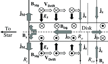
Figure 4: The $z$ component of the stellar gravitational field, $g_{z}$, interacts with the toroidal magnetic field above the disk to produce a radial drift current with a velocity $\mbox{\boldmath$V$}_{\rm Drift}$.

To illustrate how, for example, a radial, gravitational drift current could arise from the field configuration shown in Fig. 2, we note, from Brekke (1997), that the drift velocity, $V_{D}$, of a charge, $q$, subject to a force, $F_{\perp}$, perpendicular to a magnetic field, $B$, is given by

$$\mbox{\boldmath$V_{D}$}=\frac{\mbox{\boldmath$F_{\perp}$}\times\mbox{\boldmath$B$}}{qB^{2}}\ .$$ (15)

Using Eqn (15) we schematically show, in Fig. 4, how the cross product of the "wound up" toroidal field ($i.e.$, $B_{M\phi}$, produced by the disk/star current flow, $I_{M}$) and the $z$ component of the stellar gravitational force can produce a radial, gravitational drift of positively charged particles (and hence a current) above and below the disk. Other particle drifts are also possible, the gravitational drift case is shown for purposes of illustration.

It is presumed that this hypothetical ‘short-circuit’ region has an inner radius of $r=R_{t}$ and an outer radius, $R_{o}$, where $R_{o}<R_{co}$. The radial transfield current, ($j_{r}$), can interact with the toroidal field, $B_{M\phi}$. The subsequent $\mbox{\boldmath$j_{r}$}\times\mbox{\boldmath$B_{M\phi}$}$ Lorentz force is in the correct direction to power a flow away from the disk.

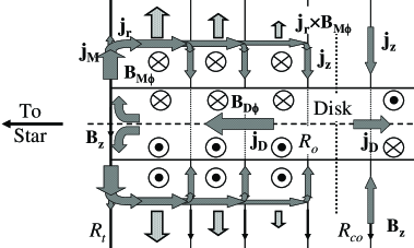
Figure 5: Even in a highly-conductive plasma, transfield currents can flow between the stellar magnetic field lines above and below the accretion disk between $R_{t}$ and $R_{o}$. The interaction between the transfield currents and the toroidal fields give rise to the $\mbox{\boldmath$j$}\times\mbox{\boldmath$B$}$ Lorentz forces, which drive the outflow

For the jet flow shown in Fig. 5, the flow can only escape the stellar magnetosphere when:

$$\frac{1}{2}\rho v^{2}\geq\frac{B(R_{t})^{2}}{2\mu_{0}}\sim\frac{B_{*}(R_{*})^{2}}{2\mu_{0}}\left(\frac{R_{*}}{R_{t}}\right)^{6}\ ,$$ (16)

where, $\rho$ is the gas mass density, $v$ the wind speed and it is assumed that the main part of the flow occurs at the inner edge of the disk ($r=R_{t}$). To find the required values of $\rho$ and $v$, we note that the velocity of the flow has to be of order the escape speed:

$$v\sim\sqrt{\frac{GM_{*}}{r}}=133\ \sqrt{\frac{\left(M_{*}/{\rm M}_{\odot}\right)}{\left(r/0.05{\rm AU}\right)}}\ {\rm km\ s}^{-1}\ .$$ (17)

Combining Eqns (16) and (17) gives

$$\rho\sim\frac{B_{*}(r)^{2}r}{\mu_{0}GM_{*}}=1.86\times 10^{-13}\times$$ (18)

$$\frac{\left(B_{*}(R_{*})/0.01{\rm T}\right)^{2}\left(R_{*}/2{\rm R}_{\odot}\right)^{6}}{\left(M_{*}/{\rm M}_{\odot}\right)\left(r/0.05{\rm AU}\right)^{5}}\ {\rm kg}\ {\rm m}^{-3}.$$

The existence of such a ‘break-out’ energy suggests the possibility of a pulsatile jet flow.

4.1 Jet Exhaust Speed

Applying Amperes Law to a thin slice (thickness $dz$) of a region above the disk gives

$$\frac{\partial B_{\phi}}{\partial z}(r,z)=-\mu_{0}j_{r}(r,z)\ .$$ (19)

As an illustrative example, we will assume a constant radial current in $z$ for $z\in[z_{0},z_{T}]$, where $z_{0}$ and $z_{T}$ are the bottom and top, respectively, of the outflow acceleration region. We denote this constant, $z$ independent, radial current density by $J_{r}$. By also assuming that $B_{\phi}(r,z_{T})=0$, we can solve Eqn (19) to obtain

$$B_{\phi}(r,z)=\mu_{0}(z_{T}-z_{0})J_{r}(r)\left(1-\frac{z-z_{0}}{z_{T}-z_{0}}\right)\ .$$ (20)

The total radial current, $I_{r}(r)$, is given by

$$I_{r}(r)=2\pi r(z_{T}-z_{0})J_{r}(r)\ .$$ (21)

Combining Eqns (20) and (21) gives

$$B_{\phi}(r,z)=\frac{\mu_{0}I_{r}(r)}{2\pi r}\left(1-\frac{z-z_{0}}{z_{T}-z_{0}}\right),\ z\in[z_{0},z_{T}]\ .$$ (22)

Liffman & Siora (1997) obtained a Bernoulli equation for the flow:

$${v^{2}\over 2}+\left(\frac{\gamma}{\gamma-1}\right)\frac{p}{\rho}+\frac{B^{2}}{\mu_{0}\rho}-\frac{GM_{*}}{\sqrt{r^{2}+z^{2}}}+\frac{GM_{*}r_{0}}{2r^{2}}=\cal{E},$$ (23)

with $\cal{E}$ the constant specific energy of the streamline flow, $\gamma$ - the ratio of specific heats, $B$ is the toroidal magnetic field, $p$ - pressure, $r_{0}$ - the initial value of $r$, and $v=\sqrt{v_{r}^{2}+v_{z}^{2}}$.

Using Eqns (22) and (23) one can obtain an expression for the exhaust speed of the jet flow, $v_{e}$:

$$v_{e}\approx\sqrt{\frac{\mu_{0}}{2\rho_{0}}}\ \frac{I_{r}(r_{0})}{\pi r_{0}}=337.3\times$$ (24)

$$\sqrt{\frac{10^{-12}\ {\rm kg}\ {\rm m}^{-3}}{\rho_{0}}}\left(\frac{I_{r}}{10^{13}\ {\rm A}}\right)\left(\frac{0.05\ {\rm AU}}{r_{0}}\right)\ {\rm km}\ {\rm s}^{-1}\ .$$

where $\rho_{0}$ is the gas density at the base of the flow. The representative values for $\rho_{0}$, $I_{r}$ and $r_{0}$, as given in Eqn (24), are obtained from Eqns (18), (11), and (1), respectively.

4.2 Radial Size of the Outflow Region

We denote by $R_{o}$ the distance from the star, where the integrated current density entering the top half of the disk ($j_{z}$ - as depicted in Fig. 5) is equal to the integrated current density returning to the disk via the stellar magnetosphere ($j_{M}$ and $j_{r}$ as in Fig. 5).

Let $I_{z}(r)$ denote the total vertical current entering the top half of the disk from the inner edge of the accretion disk, $R_{t}$, to a distance $r$ from the star:

$$I_{z}(r)=\int^{r}_{R_{t}}j_{z}(r)2\pi rdr\ .$$ (25)

Substituting Eqns (8) and (5) into Eqn (25) implies

$$I_{z}(r)=-\frac{2\pi R_{t}B_{*}(R_{t})}{\mu_{0}\beta}\times$$ (26)

$$\left(2\left(\frac{R_{t}}{R_{co}}\right)^{3/2}\left[1-\left(\frac{R_{t}}{r}\right)^{1/2}\right]-\frac{5}{4}\left[1-\left(\frac{R_{t}}{r}\right)^{2}\right]\right).$$

If we consider the case where all of the $I_{M}$ (Eqn (10)) current short circuits via the radial transfield current $j_{r}$ and then back to the disk via the field-aligned current $j_{z}$ then, for this case, $R_{o}$ is determined by equating $I_{M}$ and $I_{z}(r)$, and specifying that $r=R_{o}$. This condition implies that

$$\left(\frac{R_{t}}{R_{co}}\right)^{3/2} - 1=2\left(\frac{R_{t}}{R_{co}}\right)^{3/2}\times$$

$$\left[1-\left(\frac{R_{t}}{R_{o}}\right)^{1/2}\right]-\frac{5}{4}\left[1-\left(\frac{R_{t}}{R_{o}}\right)^{2}\right]\ .$$

We can numerically solve for $R_{o}$ in the above equation and obtain values for $(R_{o}-R_{t})/R_{co}$, which is the normalized length of the outflow region in the inner accretion disk. These results are shown in Fig. 6, where it can be seen that as the inner disk approaches the star ($R_{t}\rightarrow R_{*}$) the width of the outflow acceleration region decreases ($R_{o}\rightarrow R_{t}$). Similarly, as the inner disk approaches the co-rotation radius the width of the outflow acceleration region decreases to zero. The maximum width of the acceleration region occurs when the inner disk radius is approximately half that of the co-rotation radius. This behaviour is represented schematically in Fig. 8, , where we note that the outer radius of the outflow acceleration region is always less than the co-rotation radius ($R_{o}<R_{co}$).

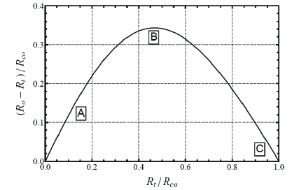
Figure 6: The length of the outflow active region of the inner disk ($R_{o}-R_{t}$) as a function of the inner truncation radius, $R_{t}$, of the disk, where both quantities are normalized to the co-rotation radius, $R_{co}$. The widths of the outflow at points A, B and C are depicted schematically in Fig. 8

4.3 Mass Ejection Rate

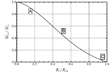
Figure 7: The ratio of outflow mass rate, $\dot{M}_{w}$, to the mass accretion rate onto a star, $\dot{M}_{a}$, versus the ratio of the inner disk truncation radius to the co-rotation radius ($R_{t}/R_{co}$). The mass flow rates of the outflow at points A, B and C are depicted schematically by the length of the arrows in Fig. 8

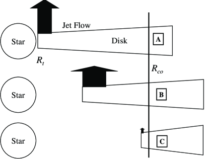
Figure 8: A schematic depiction of the mass outflow rate and the radial size of the outflow acceleration region as a function of the inner disk truncation radius, $R_{t}$, and the co-rotation radius, $R_{co}$ - indicated by the line. The length of the arrow represents the outflow mass rate, $\dot{M}_{w}$, while the width of the arrow indicates the actual, relative size of the outflow acceleration region. Case A: $R_{t}$ is small relative to $R_{co}$ and $\dot{M}_{w}\sim\dot{M}_{a}$. B: $R_{t}\sim R_{co}/2$, the outflow acceleration region is at its broadest and $\dot{M}_{w}\sim\dot{M}_{a}/2$. C: $R_{t}\sim R_{co}$ and $\dot{M}_{w}\rightarrow 0$.

From the conservation of mass, the mass ejection rate of an outflow, $\dot{M}_{w}$, is

$$\dot{M}_{w}=\rho vA\ ,$$ (28)

where $\rho$, $v$ and $A$ are, respectively, the density, speed and cross-sectional area of the outflow. Noting that

$$A=\pi(R_{o}^{2}-R_{t}^{2})$$ (29)

and using Eqns (17), (18) and (1), Eqn (28) has the form

$$\dot{M}_{w}=\frac{\dot{M}_{a}}{4}\left[\left(\frac{R_{o}}{R_{t}}\right)^{2}-1\right]$$ (30)

Using Eqns (30) and (4.2), we can compute the ratio $\dot{M}_{w}/\dot{M}_{a}$ as a function of $R_{t}/R_{co}$. These results are shown in Fig. 7, where it can be seen that when $R_{t}=R_{co}$ the high-speed outflow shuts down. On the other hand, for a fixed co-rotation radius, the mass outflow rate increases and approaches the mass accretion rate as the inner disk radius approaches the surface of the star. This behaviour is represented schematically in Fig. 8.

The observed values for the mass outflow and accretion rates are only known to order-of-magnitude values: $\dot{M}_{w}/\dot{M}_{a}\sim 0.1$ (Calvet 1997), while the modeling of T Tauri observational data gives: $R_{t}/R_{co}\approx 0.6\ {\rm to}\ 0.8\$ (Kenyon $et\ al.$ 1996). From Fig. 7, the corresponding range of values for $\dot{M}_{w}/\dot{M}_{a}$ is $\dot{M}_{w}/\dot{M}_{a}\approx 0.33\ {\rm to}\ 0.13\$. These values are consistent with the observational values.

5 Conclusions

The star-disk electric circuit arises due to the interaction of the stellar magnetosphere and the accretion disk. We have shown that the electric circuit model and standard MHD analysis give the same expressions for the disk magnetic field and the torque between the disk and the star.

We examined the hypothetical case where there is a short circuit in the star-disk circuit. This radial short circuit may be due to a gravitational drift current, which might be of sufficient magnitude to generate a non-constant bipolar outflow at the inner edge of the disk that flows in a direction roughly perpendicular to the disk.

In this model, the irregularity in the outflow arises because the outflow has to disrupt the stellar magnetic field for it to escape the stellar-disk system. The model predicts that the mass outflow rate is proportional to the total mass accretion rate in the disk. The mass outflow rate is also dependent on the position of the inner edge of the disk relative to the disk co-rotation radius. If the position of the inner edge of the disk is equal to the disk co-rotation radius, then there is little or no outflow. As the inner edge of the disk approaches the star (assuming a constant co-rotation radius) then the proportion of material going into the outflow increases, while the proportion of material accreting onto the star decreases.

References

(1) Bardou A., Heyvaerts J.: A&A 307, 1009 (1996)
(2) Brekke A. : Physics of the Upper Polar Atmosphere, Wiley (1997)
(3) Calvet N.: In Reipurth B., Bertout C. (eds) IAU Symp. 182,
Herbig-Haro Flows and the Birth of Low Mass Stars, p. 417. Kluwer, Dordrecht (1997)