How To Kill a Penguin

Abstract

Within constrained minimal-flavor-violation the large destructive flavor-changing $Z$-penguin managed to survive eradication so far. We give a incisive description of how to kill it using the precision measurements of the $Z\to b\bar{b}$ pseudo observables. The derived stringent range for the non-standard contribution to the universal Inami-Lim function $C$ leads to tight two-sided limits for the branching ratios of all $Z$-penguin dominated flavor-changing $K$- and $B$-decays.

I Introduction

The effects of new heavy particles appearing in extensions of the standard model (SM) can be accounted for at low energies in terms of effective operators. The unprecedented accuracy reached by the electroweak (EW) precision measurements performed at the high-energy colliders LEP and SLC impose stringent constraints on the coefficients of the operators entering the EW sector. Other severe constraints came in recent years from the BaBar, Belle, CDF, and DØ experiments and concern extra sources of flavor and $CP$ violation that represent a generic problem in many scenarios of new physics (NP). The most pessimistic but experimentally well supported solution to the flavor puzzle is to assume that all flavor and $CP$ violation is governed by the known structure of the SM Yukawa interactions. In these minimal-flavor-violating (MFV) Chivukula:1987py ; MFV ; D'Ambrosio:2002ex models correlations between certain flavor diagonal high-energy and flavor off-diagonal low-energy observables exist since, by construction, NP couples dominantly to the third generation. In order to simplify matters, we restrict ourselves in the following to the class of constrained MFV (CMFV) Blanke:2006ig models, i.e., scenarios that involve only SM operators, and thus consider just left-handed currents.

II General considerations

That new interactions unique to the third generation can lead to an intimate relation between the non-universal $Zb_{\scalebox{0.6}{$L$}}\bar{b}_{\scalebox{0.6}{$L$}}$ and the flavor non-diagonal $Zd^{j}_{\scalebox{0.6}{$L$}}\bar{d^{i}_{\scalebox{0.6}{$L$}}}$ vertices has been shown recently in Haisch:2007ia . Whereas the former structure is probed by the ratio of the $Z$-boson decay width into bottom quarks and the total hadronic width, $R_{b}^{0}$, the bottom quark asymmetry parameter, ${\cal A}_{b}$, and the forward-backward asymmetry for bottom quarks, $A_{\rm FB}^{0,b}$, the latter ones appear in many $K$- and $B$-decays.

In the effective field theory framework of MFV D'Ambrosio:2002ex , one can easily see how the $Zb_{\scalebox{0.6}{$L$}}\bar{b}_{\scalebox{0.6}{$L$}}$ and $Zd^{j}_{\scalebox{0.6}{$L$}}\bar{d^{i}_{\scalebox{0.6}{$L$}}}$ operators are linked together. The only relevant dimension-six contributions compatible with the flavor group of MFV stem from the $SU(2)\times U(1)$ invariant operators

$${\cal O}_{1} =i\left({\bar{Q}}_{L}Y_{U}Y_{U}^{\dagger}\gamma_{\mu}Q_{L}\right)\phi^{\dagger}D^{\mu}\phi\,,$$ (1)

$${\cal O}_{2} =i\left({\bar{Q}}_{L}Y_{U}Y_{U}^{\dagger}\tau^{a}\gamma_{\mu}Q_{L}\right)\phi^{\dagger}\tau^{a}D^{\mu}\phi\,,$$

that are built out of the quark doublets $Q_{L}$, the Higgs field $\phi$, the up-type Yukawa matrices $Y_{U}$, and the $SU(2)$ generators $\tau^{a}$. After EW symmetry breaking, ${\cal O}_{1,2}$ are responsible for both the effective $Zb_{\scalebox{0.6}{$L$}}\bar{b}_{\scalebox{0.6}{$L$}}$ and $Zd^{j}_{\scalebox{0.6}{$L$}}\bar{d^{i}_{\scalebox{0.6}{$L$}}}$ vertex. Since all up-type quark Yukawa couplings except the one of the top, $y_{t}$, are small, one has $(Y_{U}Y_{U}^{\dagger})_{ji}\sim y_{t}^{2}V_{tj}^{\ast}V_{ti}$ and only this contribution matters in Eq. (1).

Within the SM the Feynman diagrams responsible for the enhanced top correction to the $Zb_{\scalebox{0.6}{$L$}}\bar{b}_{\scalebox{0.6}{$L$}}$ coupling also generate the $Zd^{j}_{\scalebox{0.6}{$L$}}\bar{d^{i}_{\scalebox{0.6}{$L$}}}$ operators. In fact, in the limit of infinite top quark mass the corresponding amplitudes are up to Cabibbo-Kobayashi-Maskawa (CKM) factors identical. Yet there is a important difference between them. While for the physical $Z\to b\bar{b}$ decay the diagrams are evaluated on-shell, in the case of the low-energy $Z\to d^{j}\bar{d}^{i}$ transitions the amplitudes are Taylor-expanded up to zeroth order in the external momenta. As far as the momentum of the $Z$-boson is concerned the two cases correspond to $q^{2}=M_{\scriptscriptstyle Z}^{2}$ and $q^{2}=0$.

Figure 1: Relative deviations $\delta_{n}$ as a function of $M$. The solid, dashed, and dotted curve correspond to $n=1,2,$ and $3$, respectively. See text for details.

The general features of the small momentum expansion of the one-loop $Z\to b\bar{b}$ vertex can be nicely illustrated with the following simple but educated example. Consider the scalar integral

$$C_{0}=\frac{m_{3}^{2}}{i\pi^{2}}\int\!\frac{d^{4}l}{D_{1}D_{2}D_{3}}\,,\hskip 14.22636ptD_{i}=(l+p_{i})^{2}-m_{i}^{2}\,,$$ (2)

with $p_{3}=0$. Note that we have set the space-time dimension to four since the integral is finite and assumed without loss of generality $m_{3}\neq 0$.

In the limit of vanishing bottom quark mass one has for the corresponding momenta $p^{2}_{1}=p^{2}_{2}=0$. The small momentum expansion of the scalar integral $C_{0}$ then takes the form

$$C_{0}=\sum_{n=0}^{\infty}a_{n}\left(\frac{q^{2}}{m_{3}^{2}}\right)^{n}\,,$$ (3)

with $q^{2}=(p_{1}-p_{2})^{2}=-2\hskip 0.56905ptp_{1}\!\cdot\!p_{2}$. The expansion coefficients $a_{n}$ are given by Fleischer:1994ef

$$a_{n}=\frac{(-1)^{n}}{(n+1)!}\sum_{l=0}^{n}\begin{pmatrix}n\\ l\end{pmatrix}\frac{x_{1}^{l}}{l!}\frac{\partial^{l}}{\partial x_{1}^{l}}\frac{\partial^{n}}{\partial x_{2}^{n}}g(x_{1},x_{2})\,,$$ (4)

where

$$g(x_{1},x_{2})=\frac{1}{x_{1}-x_{2}}\left(\frac{x_{1}\ln x_{1}}{1-x_{1}}-\frac{x_{2}\ln x_{2}}{1-x_{2}}\right)\,,$$ (5)

and $x_{i}=m_{i}^{2}/m_{3}^{2}$. Notice that in order to properly generate the expansion coefficients $a_{n}$ one has to keep $x_{1}$ and $x_{2}$ different even in the zero or equal mass case. The corresponding limits can only be taken at the end.

To illustrate the convergence behavior of the small momentum expansion of the scalar integral in Eq. (3) for on-shell kinematics, we confine ourselves to the simplified case $m_{1}=m_{2}=M$ and $m_{3}=m_{t}$. We define

$$\delta_{n}=a_{n}\left(\frac{M_{\scriptscriptstyle Z}^{2}}{m_{t}^{2}}\right)^{n}\left(\sum_{l=0}^{n-1}a_{l}\left(\frac{M_{\scriptscriptstyle Z}^{2}}{m_{t}^{2}}\right)^{l}\right)^{-1}\,,$$ (6)

for $n=1,2,\ldots\,$. The $M$-dependence of the relative deviations $\delta_{n}$ is displayed in Fig. 1. We see that while for $M\lesssim 50\,{\rm GeV}$ higher order terms in the small momentum expansion have to be included in order to approximate the exact on-shell result accurately, in the case of $M\gtrsim 150\,{\rm GeV}$ the first correction is small and higher order terms are negligible. For the two reference scales $M=\{80,250\}\,{\rm GeV}$ one finds for the first three relative deviations $\delta_{n}$ numerically $+9.3\%$, $+1.4\%$, and $+0.3\%$, and $+1.1\%$, $+0.02\%$, $+0.00004\%$, respectively.

Of course the two reference points $M=\{80,250\}\,{\rm GeV}$ have been picked for a reason. While the former describes the situation in the SM, i.e., the exchange of two pseudo Goldstone bosons and a top quark, the latter presents a possible NP contribution involving besides the top, two heavy scalars. The above example indicates that the differences between the $Zb_{\scalebox{0.6}{$L$}}\bar{b}_{\scalebox{0.6}{$L$}}$ form factor evaluated on-shell and at zero external momenta are in general much less pronounced in models with new heavy degrees of freedom than in the SM. Given that this difference amounts to around $-30\%$ in the SM zbb , it is suggestive to assume that the scaling of NP contributions to the non-universal $Zb_{\scalebox{0.6}{$L$}}\bar{b}_{\scalebox{0.6}{$L$}}$ vertex is in general under $\pm 10\%$. This model-independent conclusion is well supported by the results of the calculations of the one-loop $Zb_{\scalebox{0.6}{$L$}}\bar{b}_{\scalebox{0.6}{$L$}}$ vertices in popular CMFV models presented in Haisch:2007ia .

III Model calculations

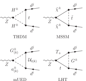
Figure 2: Examples of one-loop vertex diagrams that result in a non-universal correction to the $Z\to d^{j}\bar{d}^{i}$ transition in assorted NP scenarios with CMFV. See text for details.

The above considerations can be corroborated in another, yet model-dependent way by calculating explicitly the difference between the value of the $Zd^{j}_{\scalebox{0.6}{$L$}}\bar{d^{i}_{\scalebox{0.6}{$L$}}}$ vertex form factor evaluated on-shell and at zero external momenta. In Haisch:2007ia this has been done in four of the most popular, consistent, and phenomenologically viable scenarios of CMFV, i.e., the two-Higgs-doublet model (THDM) type I and II, the minimal-supersymmetric SM (MSSM) with MFV MFV , all for small $\tan\beta$, the minimal universal extra dimension (mUED) model Appelquist:2000nn , and the littlest Higgs model Arkani-Hamed:2002qy with $T$-parity (LHT) tparity and degenerate mirror fermions Low:2004xc . Examples of diagrams that contribute to the $Z\to d^{j}\bar{d}^{i}$ transition in these models can be seen in Fig. 2. In the following we will briefly summarize the most important findings of Haisch:2007ia .

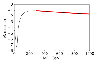
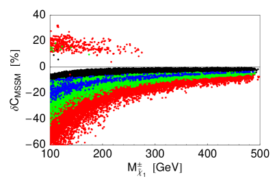
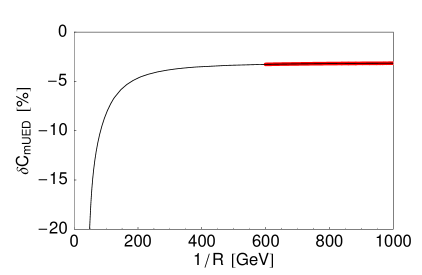
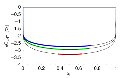
Figure 3: Relative difference $\delta C_{\rm NP}$ in the THDMs, the MSSM, the mUED, and the LHT model as a function of $M^{\pm}_{H}$, $M^{\pm}_{{\tilde{\chi}_{1}}}$, $1/R$, and $x_{L}$. Regions in the $M^{\pm}_{{\tilde{\chi}_{1}}}$–$\,\delta C_{\rm MSSM}$ plane where $|{\rm Re}\,C_{\rm MSSM}(q^{2}=0)|$ amounts to at least $2\%$, $4\%$, and $6\%$ of $|{\rm Re}\,C_{\rm SM}(q^{2}=0)|$ are indicated by the red (gray), green (light gray), and blue (dark gray) points, respectively. In the case of the LHT model the shown curves correspond, from bottom to top, to the values $f=1,1.5$, and $2\,{\rm TeV}$ of the symmetry breaking scale. See text for details.

In the limit of vanishing bottom quark mass, possible non-universal NP contributions to the renormalized off-shell $Zd^{j}_{\scalebox{0.6}{$L$}}\bar{d^{i}_{\scalebox{0.6}{$L$}}}$ vertex can be written as

$$\Gamma_{ji}^{\rm NP}=\frac{G_{F}}{\sqrt{2}}\frac{e}{\pi^{2}}M_{\scriptscriptstyle Z}^{2}\frac{c_{\scriptscriptstyle W}}{s_{\scriptscriptstyle W}}V_{tj}^{\ast}V_{ti}C_{\rm NP}(q^{2})\bar{d^{j}}_{\scalebox{0.6}{$L$}}\gamma_{\mu}{d^{i}}_{\scalebox{0.6}{$L$}}Z^{\mu}\,,$$ (7)

where $i=j=b$ and $i\neq j$ in the flavor diagonal and off-diagonal case. $G_{F}$, $e$, $s_{\scriptscriptstyle W}$, and $c_{\scriptscriptstyle W}$ denote the Fermi constant, the electromagnetic coupling constant, the sine and cosine of the weak mixing angle, respectively, while $V_{ij}$ are the corresponding CKM matrix elements.

As a measure of the relative difference between the complex valued form factor $C_{\rm NP}(q^{2})$ evaluated on-shell and at zero momentum we introduce

$$\delta C_{\rm NP}=1-\frac{{\rm Re}\,C_{\rm NP}(q^{2}=0)}{{\rm Re}\,C_{\rm NP}(q^{2}=M_{\scriptscriptstyle Z}^{2})}\,.$$ (8)

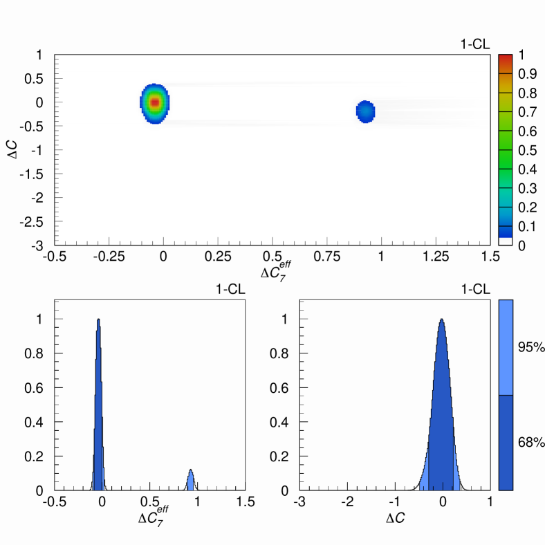
Figure 4: Constraints on $\Delta C_{7}^{\rm eff}$ and $\Delta C$ within CMFV that follow from a combination of the $Z\to b\bar{b}$ POs with the measurements of $\bar{B}\to X_{s}\gamma$ and $\bar{B}\to X_{s}l^{+}l^{-}$. The colors encode the frequentist $1-{\rm CL}$ level and the corresponding $68\%$ and $95\%$ probability regions as indicated by the bars on the right side of the panels. See text for details.

The dependence of $\delta C_{\rm NP}$ on the charged Higgs mass $M^{\pm}_{H}$, the lighter chargino mass $M^{\pm}_{{\tilde{\chi}_{1}}}$, the compactification scale $1/R$, and $x_{L}$ which parameterizes the mass of the heavy top $T_{+}$ is illustrated in Fig. 3. The allowed parameter regions after applying experimental and theoretical constraints are indicated by the colored (grayish) bands and points.

In the THDMs, the mUED, and the CMFV version of the LHT model the maximal allowed suppressions of ${\rm Re}\,C_{\rm NP}(q^{2}=M_{\scriptscriptstyle Z}^{2})$ with respect to ${\rm Re}\,C_{\rm NP}(q^{2}=0)$ amounts to less than $2\%$, $5\%$, and $4\%$, respectively. This feature confirms the general argument presented in the last section. The situation is less favorable in the case of the CMFV MSSM, since $\delta C_{\rm MSSM}$ frequently turns out to be larger than one would expected on the basis of the model-independent considerations if the masses of the lighter chargino and stop both lie in the hundred ${\rm GeV}$ range. However, the large deviation $\delta C_{\rm MSSM}$ are ultimately no cause of concern, because $|{\rm Re}\,C_{\rm MSSM}(q^{2}=0)/{\rm Re}\,C_{\rm SM}(q^{2}=0)|$ itself is always below $10\%$. In consequence, the model-independent bounds on the NP contribution to the universal $Z$-penguin function that will be derived in the next section do hold in the case of the CMFV MSSM. More details on the phenomenological analysis of $\delta C_{\rm NP}$ in the THDMs, the CMFV MSSM, the mUED, and the LHT model including the analytic expressions for the form factors $C_{\rm NP}(q^{2})$ can be found in the recent article Haisch:2007ia .

Table 1: Bounds for various rare decays in CMFV models at $95\%$ probability, the corresponding values in the SM at $68\%$ and $95\%\,{\rm CL}$, and the available experimental information. See text for details.

Observable	CMFV ($95\%\,{\rm CL}$)	SM ($68\%\,{\rm CL}$)	SM ($95\%\,{\rm CL}$)	Experiment
${\cal B}(K^{+}\to\pi^{+}\nu\bar{\nu})\times 10^{11}$	$[4.29,10.72]$	$7.15\pm 1.28$	$[5.40,9.11]$	$\left(14.7^{+13.0}_{-8.9}\right)$ kp
${\cal B}(K_{L}\to\pi^{0}\nu\bar{\nu})\times 10^{11}$	$[1.55,4.38]$	$2.79\pm 0.31$	$[2.21,3.45]$	$<2.1\times 10^{4}\;\;(90\%\,\text{CL})$ Ahn:2006uf
${\cal B}(K_{L}\to\mu^{+}\mu^{-})_{\rm SD}\times 10^{9}$	$[0.30,1.22]$	$0.70\pm 0.11$	$[0.54,0.88]$	–
${\cal B}(\bar{B}\to X_{d}\nu\bar{\nu})\times 10^{6}$	$[0.77,2.00]$	$1.34\pm 0.05$	$[1.24,1.45]$	–
${\cal B}(\bar{B}\to X_{s}\nu\bar{\nu})\times 10^{5}$	$[1.88,4.86]$	$3.27\pm 0.11$	$[3.06,3.48]$	$<64\;\;(90\%\,\text{CL})$ Barate:2000rc
${\cal B}(B_{d}\to\mu^{+}\mu^{-})\times 10^{10}$	$[0.36,2.03]$	$1.06\pm 0.16$	$[0.87,1.27]$	$<3.0\times 10^{2}\;\;(95\%\,\text{CL})$ Bernhard:2006fa
${\cal B}(B_{s}\to\mu^{+}\mu^{-})\times 10^{9}$	$[1.17,6.67]$	$3.51\pm 0.50$	$[2.92,4.13]$	$<9.3\times 10^{1}\;\;(95\%\,\text{CL})$ Sanchez:2007ew

IV Numerical analysis

Using the technique of epsilon parameters a model-independent numerical analysis of $\Delta C={\rm Re}\,C(q^{2}=0)-{\rm Re}\,C_{\rm SM}(q^{2}=0)$ is a back-on-the-envelope calculation. The variation $\epsilon_{b}^{\rm NP}=\epsilon_{b}-\epsilon_{b}^{\rm SM}$ arising from NP contributions to $Zb_{\scalebox{0.6}{$L$}}\bar{b}_{\scalebox{0.6}{$L$}}$ can be defined through the inclusive partial width of $Z\to b\bar{b}$ as follows epsilonb

$$\Gamma^{\rm NP}_{bb}=(\sqrt{2}G_{F}M_{\scriptscriptstyle Z}^{2})^{\frac{1}{2}}\,\Big{(}g_{V}^{b}(\bar{b}\gamma_{\mu}b)-g_{A}^{b}(\bar{b}\gamma_{\mu}\gamma_{5}b)\Big{)}Z^{\mu}\,,$$ (9)

where

$$\frac{g_{V}^{b}}{g_{A}^{b}}=\left(1+\frac{4s^{2}_{\scriptscriptstyle W}}{3}+\epsilon_{b}^{\rm NP}\right)\frac{g_{A}^{d}}{g_{A}^{b}}\,,\hskip 7.11317ptg_{A}^{b}=(1+\epsilon_{b}^{\rm NP})\,g_{A}^{d}\,.~{}$$ (10)

From Eqs. (7), (8), and (9) one obtains

$$\Delta C=-\frac{\pi^{2}}{\sqrt{2}G_{F}M_{\scriptscriptstyle Z}^{2}c^{2}_{\scriptscriptstyle W}}(1+\delta C_{\rm NP})\,\epsilon_{b}^{\rm NP}\,.$$ (11)

By combining experimental ewpm and theoretical uncertainties zfitter in $\epsilon_{b}$ and $\epsilon_{b}^{\rm SM}$ linearly one finds

$$\epsilon_{b}^{\rm NP}=(0.4\pm 2.5)\times 10^{-3}\,.$$ (12)

Assuming $\delta C_{\rm NP}=\pm 0.1$ one then arrives at

$$\Delta C=-0.04\pm 0.26\,,$$ (13)

which implies that large negative contributions that would reverse the sign of the SM $Z$-penguin amplitude are highly disfavored in CMFV scenarios due to the strong constraint from $R_{b}^{0}$ Haisch:2007ia . Interestingly, such a conclusion cannot be drawn by considering only flavor constraints Bobeth:2005ck , since a combination of ${\cal B}(\bar{B}\to X_{s}\gamma)$, ${\cal B}(\bar{B}\to X_{s}l^{+}l^{-})$, and ${\cal B}(K^{+}\to\pi^{+}\nu\bar{\nu})$ does not allow to distinguish the SM solution $\Delta C=0$ from the wrong-sign case $\Delta C\approx-2$ at present.

The result in Eq. (13) agrees amazingly well with the numbers of a thorough global fit to the POs $R_{b}^{0}$, ${\cal A}_{b}$, and $A_{\rm FB}^{0,b}$ ewpm and the measured $\bar{B}\to X_{s}\gamma$ bsgamma and $\bar{B}\to X_{s}l^{+}l^{-}$ bxsll BRs obtained by employing customized versions of the ZFITTER zfitter and the CKMfitter package Charles:2004jd . Neglecting contributions from EW boxes these bounds read Haisch:2007ia

$$\Delta C =-0.026\pm 0.264 \!\!(68\%\,{\rm CL})\,,$$ (14)

$$\Delta C =[-0.483,0.368] \!\!(95\%\,{\rm CL})\,.$$

The constraint on $\Delta C$ within CMFV following from the simultaneous use of $R_{b}^{0}$, ${\cal A}_{b}$, $A_{\rm FB}^{0,b}$, ${\cal B}(\bar{B}\to X_{s}\gamma)$, and ${\cal B}(\bar{B}\to X_{s}l^{+}l^{-})$ can be seen in Fig. 4.

One can also infer from this figure that two regions, resembling the two possible signs of the amplitude ${\cal A}(b\to s\gamma)\propto C_{7}^{\rm eff}(m_{b})$, satisfy all existing experimental bounds. The best fit value for $\Delta C_{7}^{\rm eff}=C_{7}^{\rm eff}(m_{b})-C_{7\,{\rm SM}}^{\rm eff}(m_{b})$ is very close to the SM point residing in the origin, while the wrong-sign solution located on the right is highly disfavored, as it corresponds to a ${\cal B}(\bar{B}\to X_{s}l^{+}l^{-})$ value considerably higher than the measurements Gambino:2004mv . The corresponding limits are Haisch:2007ia

$$\begin{gathered}\Delta C_{7}^{\rm eff}=-0.039\pm 0.043\;\;(68\%\,{\rm CL})\,,\hskip 5.69054pt\\ \Delta C_{7}^{\rm eff}=[-0.104,0.026]\,\cup\,[0.890,0.968]\;\;(95\%\,{\rm CL})\,.\hskip 5.69054pt\end{gathered}$$ (17)

Similar bounds have been presented previously in Bobeth:2005ck . Notice that since the SM prediction of ${\cal B}(\bar{B}\to X_{s}\gamma)$ bsg is now lower than the experimental world average by $1.2\hskip 1.13809pt\sigma$, extensions of the SM that predict a suppression of the $b\to s\gamma$ amplitude are strongly constrained. In particular, even the SM point $\Delta C_{7}^{\rm eff}=0$ is almost disfavored at $68\%\,{\rm CL}$ by the global fit.

The stringent bound on the NP contribution $\Delta C$ given in Eq. (14) translates into tight two-sided limits for the BRs of all $Z$-penguin dominated flavor-changing $K$- and $B$-decays as shown in Tab. 1. A strong violation of any of the bounds by future measurements will imply a failure of the CMFV assumption, signaling either the presence of new effective operators and/or new flavor and $CP$ violation. A way to evade the given limits is the presence of sizable corrections $\delta C_{\rm NP}$ and/or box contributions. While these possibilities cannot be fully excluded, general arguments and explicit calculations indicate that they are both difficult to realize in the CMFV framework.

V Conclusions

R.I.P. large destructive CMFV $Z$-penguin!

- (1) R. S. Chivukula and H. Georgi, Phys. Lett. B 188, 99 (1987).
- (2) E. Gabrielli and G. F. Giudice, Nucl. Phys. B 433, 3 (1995) [Erratum-ibid. B 507, 549 (1997)]; A. Ali and D. London, Eur. Phys. J. C 9, 687 (1999); A. J. Buras et al., Phys. Lett. B 500, 161 (2001).
- (3) G. D’Ambrosio et al., Nucl. Phys. B 645, 155 (2002).
- (4) M. Blanke et al., JHEP 0610, 003 (2006) and references therein.
- (5) U. Haisch and A. Weiler, 0706.2054 [hep-ph].
- (6) J. Fleischer and O. V. Tarasov, Z. Phys. C 64, 413 (1994).
- (7) G. Mann and T. Riemann, Annalen Phys. 40, 334 (1984); J. Bernabeu, A. Pich and A. Santamaria, Phys. Lett. B 200, 569 (1988).
- (8) T. Appelquist, H. C. Cheng and B. A. Dobrescu, Phys. Rev. D 64, 035002 (2001).
- (9) N. Arkani-Hamed et al., JHEP 0207, 034 (2002).
- (10) H. C. Cheng and I. Low, JHEP 0309, 051 (2003) and 0408, 061 (2004).
- (11) I. Low, JHEP 0410, 067 (2004).
- (12) G. Altarelli, R. Barbieri and F. Caravaglios, Nucl. Phys. B 405, 3 (1993) and Phys. Lett. B 314, 357 (1993).
- (13) S. Schael et al., Phys. Rept. 427, 257 (2006).
- (14) C. Bobeth et al., Nucl. Phys. B 726, 252 (2005).
- (15) D. Y. Bardin et al., Comput. Phys. Commun. 133, 229 (2001); A. B. Arbuzov et al., Comput. Phys. Commun. 174, 728 (2006) and http://www-zeuthen.desy.de/theory/research/zfitter/index.html.
- (16) M. Misiak et al., Phys. Rev. Lett. 98, 022002 (2007); M. Misiak and M. Steinhauser, Nucl. Phys. B 764, 62 (2007).
- (17) S. Chen et al. [CLEO Collaboration], Phys. Rev. Lett. 87, 251807 (2001); P. Koppenburg et al. [Belle Collaboration], Phys. Rev. Lett. 93, 061803 (2004); B. Aubert et al. [BaBar Collaboration], Phys. Rev. Lett. 97, 171803 (2006).
- (18) B. Aubert et al. [BaBar Collaboration], Phys. Rev. Lett. 93, 081802 (2004); K. Abe et al. [Belle Collaboration], hep-ex/0408119.
- (19) J. Charles et al. [CKMfitter Group], Eur. Phys. J. C 41, 1 (2005) and http://ckmfitter.in2p3.fr/.
- (20) P. Gambino, U. Haisch and M. Misiak, Phys. Rev. Lett. 94, 061803 (2005).
- (21) S. C. Adler et al. [E787 Collaboration], Phys. Rev. Lett. 79, 2204 (1997), 84, 3768 (2000), 88, 041803 (2002) and Phys. Rev. D 70, 037102 (2004); V. V. Anisimovsky et al. [E949 Collaboration], Phys. Rev. Lett. 93, 031801 (2004).
- (22) J. K. Ahn et al. [E391a Collaboration], Phys. Rev. D 74, 051105 (2006) [Erratum-ibid. 74, 079901 (2006)].
- (23) R. Barate et al. [ALEPH Collaboration], Eur. Phys. J. C 19, 213 (2001).
- (24) R. P. Bernhard, hep-ex/0605065.
- (25) A. Sanchez-Hernandez, talk given at Rencontres de Moriond “Electroweak interactions and Unified theories”, La Thuile, Italy, March 10-17, 2007, http://moriond.in2p3.fr/.