Rotational dynamics of a superhelix towed in a Stokes fluid

Abstract

Motivated by the intriguing motility of spirochetes (helically-shaped bacteria that screw through viscous fluids due to the action of internal periplasmic flagella), we examine the fundamental fluid dynamics of superhelices translating and rotating in a Stokes fluid. A superhelical structure may be thought of as a helix whose axial centerline is not straight, but also a helix. We examine the particular case where these two superimposed helices have different handedness, and employ a combination of experimental, analytic, and computational methods to determine the rotational velocity of superhelical bodies being towed through a very viscous fluid. We find that the direction and rate of the rotation of the body is a result of competition between the two superimposed helices; for small axial helix amplitude, the body dynamics is controlled by the short-pitched helix, while there is a cross-over at larger amplitude to control by the axial helix. We find far better, and excellent, agreement of our experimental results with numerical computations based upon the method of Regularized Stokeslets than upon the predictions of classical resistive force theory.

I Introduction

The study of swimming micro-organisms, including bacteria, has long been of scientific interest Taylor52 ; Berg73 ; Lighthill76 . Bacteria swim by the action of rotating, helical flagella driven by reversible rotary motors embedded in the cell wall Berg73 . Typically, these flagella visibly emanate from the cell body. The external flagella of rod-shaped bacteria, such as E. coli, form a coherent helical bundle when rotating counter-clockwise, causing forward swimming. When these flagella rotate in the opposite direction, the flagellar bundle unravels, causing the cell to tumble. This run and tumble mechanism allows a bacterium to swim up a chemo-attractant gradient as it senses temporal changes in concentration Brownberg ; Macnab . Many studies have focused on the fundamental fluid mechanics surrounding this locomotion affected by a simple helical flagellum attached to and extruded from the cell body Lighthill76 ; Purcell97 . Recently, there have been additional studies that investigate the hydrodynamics of flagellar bundling Powers ; Flores .

In contrast, swimming bacteria with more complicated body-flagella arrangements are less studied. Spirochetes are such a group of bacteria. They have a helically-shaped cell body CDMF84 ; Lepto , and although they also swim due to the action of rotating flagella, these do not visibly project outward from their cell body. Instead, the cell body is surrounded by an outer sheath, and it is within this periplasmic space that rotation of periplasmic flagella (PFs) occurs. These helical periplasmic flagella emanate from each end of the cell body, but rather than extend outwards, they wrap back around the helical cell body. In the case of Leptospiracaeae, there are two PFs, one emerging from each end of the cell body, that do not overlap in the center of the cell. Rotation of each flagella is achieved by a rotary motor embedded in the cell body. The shapes of both ends of the helical cell body are then determined by the intrinsic helical structure of the periplasmic flagella, as well as their direction of rotation. During forward swimming, L. illini exhibit an anterior region that is superhelical, due to this interplay of helical cell body and helical flagellum Lepto . In fact, the handedness of these two helical structures are opposite, with the flagellum (axial helix) exhibiting a much larger pitch than the cell body helix.

The overall swimming dynamics of spirochetes involves non-steady coupling of the complex geometry of the cell body, the flexible outer sheath, and the counter-rotation of the cell body with the internal flagella. However, a natural question is how the effectiveness of spirochete locomotion depends upon the detailed superhelical geometry of the anterior region of the bacterium. With this as motivation, we present here a careful study of the fundamental fluid mechanics of superhelical bodies translating and rotating through highly viscous fluids. We extend the classical analytic and experimental results of Purcell Purcell97 and the numerical results of Cortez et al. Cortez05 performed for regular helices. In addition, we offer coordinated laboratory and computational experiments as validation of the method of Regularized Stokeslets for zero Reynolds number flow coupled with an immersed, geometrically complex body. This method uses modified expressions for the Stokeslet in which the singularity has been mollified. The regularized expression is derived as the exact solution to the Stokes equations consistent with forces given by regularized delta functions.

We focus on a typical body that is a short-pitched helix whose axis is itself shaped as a helix of larger pitch and opposite handedness. In the following sections, we describe the experimental set-up as well as the construction of these superhelical bodies. We experimentally measure the rotational velocities of the bodies as they are towed with a constant translational velocity through a very viscous fluid. Note that rotational and translational velocities should be proportional, with the constant of proportionality (resistance coefficient) dependent upon the body geometry. The rotational velocities corresponding to translational velocities are also predicted analytically using resistive force theory, as well as using the method of Regularized Stokeslets Cortez01 ; Cortez05 . We find compatible behavior between experiments and the resistive force theory, but excellent quantitative agreement between experiments and the method of Regularized Stokeslets.

II Superhelix construction

A superhelix is formed from a copper wire chosen to be sufficiently malleable to deform into a desired shape, but rigid enough not to deform as it moves through the viscous fluid. The superhelix is made in two steps (see Fig. 1(b)). First, a copper wire of diameter 0.55 mm is wound tightly in a clockwise direction up a rod of diameter 3.15 mm, forming a tight coil. After removing the coil from the rod, we stretch it out into a smaller radius, larger pitch helix, simply by pulling the ends of the coil away from each other. The axial helix is made in the same manner, but we use lead wire of a thicker diameter (3.15 mm) and a larger rod (4.7 mm diameter). The most important difference between the two helices is handedness; the axial helix is wound counter-clockwise up the rod, whereas the small helix is wound clockwise. Once the parameters of the small and axial helices are measured, the axial helix is threaded through the small helix, forming a superhelix, i.e. the small helix is placed back on a rod that has been distorted into a helical shape. The last step is to remove the axial helix. This is done by simply rotating the axial helix while keeping the superhelix fixed.

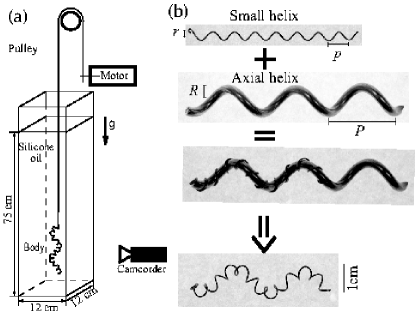
Figure 1: (a) Schematic of experimental setup. A motor pulls a rigid body through silicon oil, a highly viscous Stokes fluid ($\nu$ = 10,000 cSt) (b) Procedure for making superhelix.

The defining geometric parameters of the superhelix are the radius $r$ and pitch $p$ of the small helix, and the radius $R$ and pitch $P$ of the axial helix (see Fig. 1). For $R=0$ or $P=\infty$, the superhelix reduces to a regular helix. In our experiments, two different sets of small helices are used. The corresponding geometric parameters of these small helices are the pitch ($5.58\pm 0.25$ mm; Set I and $5.04\pm 0.36$ mm; Set II) and radius ($1.91\pm 0.14$ mm; Set I and $1.75\pm 0.21$ mm; Set II). The small (less than 12%) variations of pitch and radius are presumably due to mechanical relaxation of material when it is pulled off the axial helix. Seven different axial helices are prepared from the same initial coil (see Fig. 2).

We now construct a mathematical representation of the superhelix. The coordinates of an axial helix are ${\mbox{$X$}}=(R\cos(Kz),R\sin(Kz),z)$, where $K=\frac{2\pi}{R}$. The distance measured along this helix is linearly proportional to the axial distance $z(=\alpha s)$. The unit vector tangential to the axial helix is $\hat{{\mbox{$t$}}}_{A}={\partial{\mbox{$X$}}}/{\partial s}$. The principal normal vector is $\hat{{\mbox{$n$}}}_{A}=(-\cos(Kz),-\sin(Kz),0)$ and the binormal is $\hat{{\mbox{$b$}}}_{A}=\hat{{\mbox{$t$}}}_{A}\times\hat{{\mbox{$n$}}}_{A}=\alpha(\sin(Kz),-\cos(Kz),RK)$. Since $\hat{{\mbox{$t$}}}_{A}$ is a unit vector sets $\alpha$ as:

$$\alpha^{2}(R^{2}K^{2}+1) = 1\,.$$ (1)

The coordinates of the one-dimensional curve describing the superhelix are:

$${{\mbox{$R$}}}(s)=(R_{x},R_{y},R_{z})$$

$$={{\mbox{$X$}}}(s)+r\cos(ks)\hat{{{\mbox{$n$}}}}_{A}+r\sin(ks)\hat{{\mbox{$b$}}}_{A}\,.$$ (2)

Recall that the actual superhelices have nonzero thickness (the diameter of the copper wire), and hence are true three-dimensional structures.

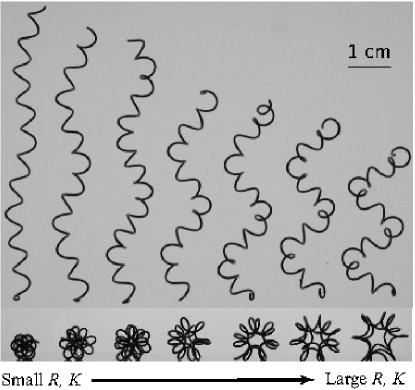
Figure 2: Seven superhelices with increasing axial helix radius (from left to right). The upper panel is the side view and the lower panel is the axial view.

III Experiment

The classical experiments of Purcell, elaborated on in Purcell97 , examined the relationship between angular and translational velocities of helical objects at very low Reynolds numbers. Here we extend these experiments to the superhelical objects described above. The experimental setup was originally designed for sedimentation experiments Jung06 (see Fig. 1(a)). A tall transparent container is filled with silicone oil with large viscosity ($\nu=10^{4}$ cS, $\rho=0.98$ g/cm³). The oil behaves as a Newtonian fluid in the regime of interest here. Rather than allowing the superhelical object to descend by gravity, our experiment is designed to measure its rotational speed as it is towed up through the viscous column of fluid at a specified translational speed. To drag the superhelix, a small hook ($\sim$ 2 mm) is used to attach the superhelix to a thread from a motor. Note that the dimensions of this hook are quite small compared to the superhelix length ($\sim 4$ cm). By experimentally testing with an axisymmetric body (sphere), we found that this towing system (the thread plus the motor), does not produce any torque on the body.

The superhelix is initially positioned near the bottom of the container, then is dragged upwards by the motor (Clifton Precision-North) at constant speed. In the intermediate region in the container, steady state motion (constant translational velocity, rotational velocity, and drag force) is assumed. The superhelix positions, orientations, and velocities are measured from a 30 frames per second video stream of the camcorder. The translational velocity in our experiments varies by changing power input to the motor. We have chosen a velocity range of 3-10 cm/s. Below 3 cm/s, the step motor produces non-uniform pulsed axle rotations, which lead to irregular translational velocity. The Reynolds number based upon the towing velocity and radius of the superhelical structure (1 cm) is at most:

$$Re=\frac{UR}{\nu}\sim 0.1\,.$$ (3)

We assume therefore that the steady Stokes equations govern the fluid mechanics of the translating superhelix. Within this translational velocity range, a linear relationship between rotational velocity $\Omega$ and translational velocity $U$ is observed (see Fig. 3).

A translating helix in a viscous solution rotates in the direction which it screws in. Following this rule, the small (straight) helix in our experiments would rotate clockwise and the axial (straight) helix would rotate counter-clockwise when viewed from above. In Purcell’s work Purcell97 , the jointed structure built by connecting two helices of opposite handedness, otherwise identical, showed no rotation during its sedimentation. The superhelix of interest here is the superposition of two helices with opposite handedness. The inherent rotational directions of these superimposed helices are in competition. For very small values of the non-dimensional parameter $RK$ of the axial helix, the superhelical structure reverts to the straight small helix, and would rotate clockwise. One expects that for larger values of the parameter $RK$, the axial helix would be dominant, and the superhelical structure would rotate counter-clockwise. For some critical value of $RK$, we would expect a transition in direction, and hence, a structure that would show no rotation as it is towed through the fluid. We performed experiments that systematically varied $RK$, and observed this expected change in rotational direction. Fig. 4 shows the ratio of angular velocity to translational velocity as a function of $RK$, for the two different sets of superhelices (Sets I & II). Positive rotational rate is clockwise, and negative is counter-clockwise. In each set of experiments, the measured ratio is depicted by triangles. In the next sections, we describe mathematical formulations that model these observations.

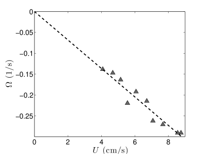
Figure 3: A linear relationship between the translational velocity and rotational frequency of a superhelix ($r=0.89$ mm, $R=4.62$ mm, $p=5.5$ mm, and $P=19.4$ mm). Triangles are from experimental observations. Dashed line is a least-square fit of experimental data.

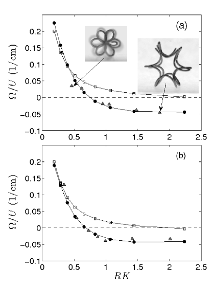
Figure 4: Ratio of angular velocity to translational towing velocity. Triangles are values measured experimentally. Circles connected by lines are values predicted using the method of Regularized Stokeslets. Squares are values predicted using resistive force theory. (a) Superhelices of Set I. Positive rotational rate is clockwise and negative rate is counter-clockwise. Rotational direction changes around 0.7 for $RK$. (b) Superhelices for Set II. Same transition also occurs around 0.7 for $RK$.

IV Numerical Results

IV.1 Regularized Stokeslets

We assume that the superhelix is a rigid body moving in a Stokes fluid. The governing equations of motion are:

$$-{{\mbox{$\nabla$}}}p+\mu\nabla^{2}{{\mbox{$u$}}}=0,~{}\nabla\cdot{\mbox{$u$}}=0\,.$$ (4)

The total hydrodynamic force and torque exerted by the superhelix (with surface $\partial D$) on the surrounding fluid is:

$$\begin{array}[]{rcl}{\bf F}&=&\int\limits_{{\bf x}\in\partial D}{{\bf f}({\bf x})d{\bf x}},\end{array}$$ (5)

$$\begin{array}[]{rcl}{\bf L}&=&\int\limits_{{\bf x}\in\partial D}{({\bf x}-{\bf x_{0}})\times{\bf f}({\bf x})d{\bf x}}.\end{array}$$ (6)

where ${\bf f}$ is the surface traction.

A solution to the Stokes equations in 3D with a point force centered at ${\mbox{$x$}}_{0}$ is the classical Stokeslet Poz . Due to the linearity of the Stokes equations, superposition of these fundamental solutions allows the construction of the velocity field induced by a distribution of point forces. The method of Regularized Stokeslets eases the evaluation of integrals with singular kernels by replacing the delta distribution of forces by a smooth, localized distribution Cortez01 ; Cortez05 . The force ${\mbox{$f$}}={\mbox{$f$}}({\mbox{$x$}}_{0})\delta({\mbox{$x$}}-{\mbox{$x$}}_{0})$ is replaced by ${\mbox{$f$}}={\mbox{$f$}}({\mbox{$x$}}_{0})\phi_{\epsilon}({\mbox{$x$}}-{\mbox{$x$}}_{0})$ where $\phi_{\epsilon}$ is a cutoff, or blob, function with integral one. This blob function is an approximation to the 3D Dirac delta function, with $\epsilon$ a small parameter. Following Cortez05 , we choose

$$\phi_{\epsilon}({\mbox{$x$}}-{\mbox{$x$}}_{0})=\frac{15\epsilon^{4}}{8\pi(\|{\mbox{$x$}}-{\mbox{$x$}}_{0}\|^{2}+\epsilon^{2})^{7/2}}\,.$$ (7)

For $N$ regularized point forces distributed on the surface of a body in rigid rotation and translation, the fluid velocity at any point $x$ is evaluated as

$${8\pi\mu}{u}_{i}({\mbox{$x$}})=\sum_{j}\sum_{n=1}^{N}S^{\epsilon}_{ij}({\mbox{$x$}},{\mbox{$x$}}_{n}){f}_{j}({\mbox{$x$}}_{n})$$ (8)

For the given cutoff function, the kernel $S$ is

$$S^{\epsilon}_{ij}({\mbox{$x$}},{\mbox{$x$}}_{n})=\delta_{ij}\frac{r^{2}+2\epsilon^{2}}{(r^{2}+\epsilon^{2})^{3/2}}+\frac{(x_{i}-x_{n,i})(x_{j}-x_{n,j})}{(r^{2}+\epsilon^{2})^{3/2}}\,$$ (9)

where $r=\|{\mbox{$x$}}-{\mbox{$x$}}_{n}\|$.

Note that evaluating equation (8) at each of the $N$ points of the superhelix surface gives us a linear relation between the velocities and the forces exerted at these points. The matrix $S^{\epsilon}_{ij}$, for a given cutoff parameter $\epsilon$ depends only upon the geometry of the superhelix.

For a rigid body moving in a Stokes flow, there is a linear relationship between the total hydrodynamic force and torque and the translational and rotational velocity of the body Purcell97 . Following Purcell97 ; Cortez05 , we focus on the $z$-components of total hydrodynamic force $F$ and torque $L$, along with the $z$-component of translational velocity $U$, and rotational velocity about the $z$-axis $\Omega$. These are related by resistance (or propulsion) coefficients:

$$\left(\begin{array}[]{c}F\\ L\end{array}\right)=\mu\left(\begin{array}[]{cc}A&B\\ B&D\end{array}\right)\left(\begin{array}[]{c}U\\ \Omega\end{array}\right)\,.$$ (10)

Here $A$, $B$, and $D$ depend only upon the geometry of the object.

In order to compute these coefficients, we discretize the cross sections of the copper wire using six azimuthal grid points. We choose a cutoff parameter $\epsilon$ on the order of the distance between discrete points (see Cortez05 for details). At each point on this discretized superhelix, we impose a unit translational velocity and zero rotational velocity in the $z$-direction. We use the Regularized Stokeslet linear relation (8) to solve for the forces on the superhelix that produced this velocity. We then evaluate the integrals for total force $F$ and total torque $L$ in equations (5, 6) above. Using the linear equations (10), we compute the resistance coefficients $A,B$. Similarly, we can compute $D$ by imposing a unit rotational velocity and zero translational velocity.

These resistance coefficients allow us to predict the ratio of rotational velocity to translational velocity in our torque-free experiments described above, as

$$\frac{\Omega}{U}=-\frac{B}{D}\,.$$ (11)

Figure 4 shows the Regularized Stokelet predictions (circles) of these ratios for both sets of superhelices. The agreement with experimental data is excellent. Indeed, the transition from clockwise to counter-clockwise rotation is captured very precisely.

IV.2 Resistive Force Theory

Resistive force theory Hancock53 ; Gray55 is widely used to give an approximate description on a slender body moving in a viscous fluid. However, the non-local interactions of stress along the body are not taken into account. To see how important this non-local interaction is, we analytically estimate the ratio of angular to translational velocities in this section, and compare the predictions with experiment and the numerical calculations using regularized Stokeslets.

The Stokes drag force is proportional to its velocity as ${\mbox{$f$}}=C_{t}({\mbox{$u$}}\cdot\hat{t})\hat{t}+C_{n}({\mbox{$u$}}\cdot\hat{n})\hat{n}$ where $\hat{t}$ and $\hat{n}$ are tangential and normal directions, and $C_{t}$ and $C_{n}$ are drag coefficients. The normal direction is arbitrary, but, uniquely determined if the motion is given.

First, we consider pure body-rotation about the $z$-axis. The body velocity is ${\mbox{$u$}}={\mbox{$R$}}_{\perp}\times{\mbox{$\Omega$}}=\Omega\,(R_{y},-R_{x},0)=\Omega R_{\perp}\hat{u}$ where ${\mbox{$R$}}_{\perp}=(R_{x},R_{y},0)$, ${R}_{\perp}=\|{\mbox{$R$}}_{\perp}\|$, $\hat{u}=\hat{R}\times\hat{z}$, and ${\mbox{$\Omega$}}=\Omega\hat{z}$. The angle $\psi$ between the direction of motion and the tangential of the body is expressed by the superhelix coordinates as $\hat{u}\cdot\hat{t}=\cos\psi=(R_{y}\partial_{s}R_{x}-R_{x}\partial_{s}R_{y})/R_{\perp}$ where $\hat{t}=R_{s}$. Similarly, $\hat{u}\cdot\hat{n}=\sin\psi$.

Using the vector relation ($({\mbox{$A$}}\times{\mbox{$B$}})\cdot{\mbox{$C$}}=-({\mbox{$A$}}\times{\mbox{$C$}})\cdot{\mbox{$B$}}$), the $z$-component torques associated with forces are

$$L_{z}(s) = ({\mbox{$R$}}\times{\mbox{$f$}})\cdot\hat{z}$$ (12)

$$= C_{t}({\mbox{$u$}}\cdot\hat{t})({\mbox{$R$}}\times\hat{t})\cdot\hat{z}+C_{n}({\mbox{$u$}}\cdot\hat{n})({\mbox{$R$}}\times\hat{n})\cdot\hat{z}$$

$$= -C_{t}({\mbox{$u$}}\cdot\hat{t})({\mbox{$R$}}\times\hat{z})\cdot\hat{t}-C_{n}({\mbox{$u$}}\cdot\hat{n})({\mbox{$R$}}\times\hat{z})\cdot\hat{n}$$

$$= -\Omega R_{\perp}^{2}(C_{t}\cos^{2}\psi+C_{n}\sin^{2}\psi)\,,$$

and the total torque due to its rotational motion is

$$L_{z}^{(Rotation)}=\int L_{z}(s)ds$$

$$=-\Omega\int R_{\perp}^{2}\left[C_{t}\cos^{2}\psi+C_{n}\sin^{2}\psi\right]ds\,.~{}~{}$$ (13)

Similarly, to total torque associated with the pure translation ${\mbox{$u$}}=(0,0,U)=U\hat{z}$ is:

$$L_{z}^{(Translation)}=U\int(C_{n}-C_{t})(\partial_{s}R_{z})R_{\perp}\cos\psi ds\,.$$ (14)

Decoupling the body motion into a pure rotation and a pure translation, the $z$-component of total torque on the body is expressed as

$$L_{z}=L_{z}^{(Translation)}+L_{z}^{(Rotation)}\,.$$ (15)

In our experiments, we do not apply any external torque. Balancing two torques gives an expression for the ratio of angular velocity to translational velocity as

$$L_{z}^{(Translation)}=-L_{z}^{(Rotation)}$$ (16)

$$\Rightarrow \frac{\Omega}{U}=\frac{\int(C_{n}-C_{t})(\partial_{s}R_{z})R_{\perp}\cos\psi ds}{\int R_{\perp}^{2}\left[C_{t}\cos^{2}\psi+C_{n}\sin^{2}\psi\right]ds}\,.$$

Note that this ratio of velocities depends only upon the ratio of drag coefficients $\frac{C_{n}}{C_{t}}$. Evaluating numerically these integrals, and using $R$ and $C_{n}=2C_{t}$ (the leading order result of slender-body theory), $\Omega/U$ is plotted as squares in Fig. 4.

The slope ($-B/D$) in the relation (11) is measured in experiments by using a least-squares fit of the data (see Fig. 3). Although the resistive force theory predictions of $\Omega/U$ show the same general trend as the experimental measurements, the quantitative agreement is quite poor, and the transition from clockwise to counter-clockwise rotation is not captured.

V Conclusion

In conclusion, we have studied the rotational dynamics of superhelices built out of superimposed helices of opposite handedness in a viscous fluid. As the radius of the axial helix increases, we have observed the transition of rotational direction to the natural direction of rotation of the axial helix. The rotational velocities corresponding to translational velocities are also predicted semi-analytically using resistive force theory, as well as numerically, using the method of Regularized Stokeslets Cortez01 ; Cortez05 . We see that although there is qualitative agreement between experiments and resistive force theory, for larger radii of the axial helix, the predicted ratios of rotation to translational velocities differ from experimental results by more than one hundred percent, and show the incorrect direction of rotation. In contrast, the easily implemented computational framework of Regularized Stokeslets demonstrates excellent quantitative agreement with experiments.

While this study is motivated by the fascinating geometry of spirochetes, we recognize that the rotation of the anterior superhelix of a spirochete is not due to an imposed rotation about a vertical axis, but due to the counter-rotation of the periplasmic flagellum (that determines the axial helix), against the cell body (the small helix). The fluid mechanic implications of this counter-rotation that govern spirochete motility is examined in mcgf07 .

We thank J. Zhang, E. Kim, A. Medovikov, R. Cortez for helpful discussions. This work was partially supported by by the DOE (Grant No. DE-FG02- 88ER25053) and NSF DMS 0201063.

References

- (1) G. I. Taylor, “The action of waving cylindrical tails in propelling microscopic organisms,” Proc. Royal Soc. London A 211, 225–239 (1952).
- (2) H. C. Berg,“Bacteria swim by rotating their flagellar filaments,” Nature 245, 380–382 (1973).
- (3) J. Lighthill, “Flagellar Hydrodynamics,” SIAM review 18, 161–230 (1976).
- (4) D. Brown and H. C. Berg, “Temporal stimulation of chemotaxis in Escherichia coli,” Proc. Natl. Acad. Sci. U.S.A., 71, 1388 (1974).
- (5) R. M. MacNab and D. E. Koshland, “The gradient-sensing mechanism in bacterial chemotaxis,” Proc. Natl. Acad. Sci. U.S.A., 69, 2509 (1972).
- (6) E. Purcell, “The efficiency of propulsion by a rotating flagellum,” Proc. Natl. Acad. Sci. U.S.A. 94, 11307 (1997).
- (7) M. Kim, J. Bird, A. Van Parys, K. Breuer, T. Powers, “A macroscopic scale model of bacterial flagellar bundling,” Proc. Natl. Acad. Sci. U.S.A., 100, 15481-15485 (2003).
- (8) H. Flores, E. Lobaton, S. Mendez-Diez, S. Tlupova, R. Cortez, “A study of baterial flagellar bundling ”, Bull. Math. Biol., 67, 137-168 (2005).
- (9) N. W. Charon, G. R. Daughtry, R. S. McCuskey, and G. N. Franz, “Microcinematographic analysis of Tethered Leptospira illini”, J. Bacter., 160 , 1067-1073 (1984).
- (10) S. Goldstein and N. Charon, “Multiple-exposure photographic analysis of a motile spirochete”, Proc. Natl. Acad. Sci. U.S.A., 87, 4895-4899 (1990).
- (11) R. Cortez, L. Fauci, and A. Medovikov, “The method of Regularized Stokeslets in three dimensions: Analysis, validation, and application to helical swimming,” Phys. Fluids 17, 031504 (2005).
- (12) R. Cortez, “The method of Regularized Stokeslets,” SIAM J. Sci. Comput. (USA) 23, 1204 (2001).
- (13) S. Jung, S. E. Spagnolie, K. Prikh, M. Shelley and A.-K. Tornberg “Periodic sedimentation in a Stokesian fluid,” Phys. Rev. E 74, 035302(R) (2006).
- (14) C. Pozrikidis, “Boundary integral and singularity methods for linearized viscous flow,” Cambridge University Press, Cambridge (1992).
- (15) G. J. Hancock, “The self-propulsion of microscopic organisms through liquids.” Proc. R. Soc. Lond. A 127, 96–121 (1953).
- (16) J. Gray and G. J. Hancock, “The propulsion of sea-urchin spermatozoa” J. Exp. Biol. 32, 802–814 (1955).
- (17) A. Medovikov, R. Cortez, S. Goldstein, L. Fauci, “Fluid mechanics of spirochete motility”, submitted (2007).