Hidden Structure in Protein Energy Landscapes

Abstract

Inherent structure theory is used to discover strong connections between simple characteristics of protein structure and the energy landscape of a G$\bar{\bf\sf o}$ model. The potential energies and vibrational free energies of inherent structures are highly correlated, and both reflect simple measures of networks of native contacts. These connections have important consequences for models of protein dynamics and thermodynamics.

Protein activity is controlled by dynamical transitions among conformational substates Frauenfelder and Wolynes (1985); the transitions may be understood in terms of motions on an energy landscape Frauenfelder et al. (1991). Substates correspond to local minima in the energy landscape, and transitions correspond to the hurdling of barriers between minima. Interestingly, the protein energy landscape resembles that of glasses Ansari et al. (1985).

Spin-glass models have yielded insight into properties of protein energy landscapes Bryngelson and Wolynes (1987); Stein (1985) and the kinetics of protein folding Bryngelson and Wolynes (1989). The main motivation for using spin-glass models rather than structural-glass models is that spin-glass models are more analytically tractable; however, it has long been recognized that structural-glass models might be better-suited to describe proteins Stein (1985). Indeed, protein unfolding has been characterized as a rigidity transformation that is similar to those seen in network glasses Rader et al. (2002).

Structural-glass-forming liquids have been fruitfully characterized using inherent structure (IS) theory Stillinger and Weber (1982, 1984), which treats the energy landscape as a set of discrete basins that are separated by saddles. Each basin contains a local minimum, called an inherent structure, which is analogous to a protein conformational substate. The dynamics are then naturally described as vibrations about local minima, punctuated by transitions between neighboring basins. A key assumption in IS theory is that vibrations are similar about minima with the same potential energy; however, importantly, IS theory allows for diversity among vibrations that have different potential energies.

Guo and Thirumalai Guo and Thirumalai (1996) have used IS theory to analyze fluctuations in the neighborhood of the native state of a coarse-grained model of a designed four-helix bundle protein. Baumketner, Shea, and Hiwatari Baumketner et al. (2003) have applied IS theory to study the glass transition in a coarse-grained model of a 16-residue polypeptide; by IS analysis of molecular dynamics trajectories, they demonstrated the ability to rigorously calculate the glass transition temperature due to freezing in the native-state basin. In a more recent study, Nakagawa & Peyrard Nakagawa and Peyrard (2006) used IS theory to analyze the energy landscape of a protein G B1 domain using a coarse-grained model, finding that the density of minima increases exponentially with the energy. Importantly, their analysis relied on an assumption that vibrations are the same about all potential energy minima. However, because proteins become less rigid as noncovalent bonds are broken Rader et al. (2002), vibrations are expected to be different for different minima, especially for minima with different potential energies. Diversity in vibrations not only would change the density of minima, but also would have important implications for the kinetics of transitions among conformational substates Frauenfelder and Wolynes (1985); however, if vibrations are the same for different minima, their role in determining the kinetics of transitions would be trivial.

To characterize the diversity in vibrations among different protein inherent structures, we used IS theory to analyze a coarse-grained G$\bar{\rm o}$ model of the same protein fragment considered by Nakagawa & Peyrard Nakagawa and Peyrard (2006): GB1, a protein G B1 domain (Protein Data Bank Berman et al. (2000) entry 2GB1 Gronenborn et al. (1991)). GB1 has 56 amino acids and consists of a four-stranded $\beta$-sheet packed against a single helix.

A configuration $x$ is represented by the set of ${\rm C}_{\alpha}$ positions, and the G$\bar{\rm o}$ model potential energy $U(x)$ for ${\rm C}_{\alpha}$ configurations $x$ of all proteins is similar to that used by the GB1 studies in Refs. Karanicolas and Brooks (2002) and Nakagawa and Peyrard (2006):

$$U(x) = \sum_{i=1}^{N-1}{K_{b}\over 2}\left(r_{i}-r_{i,0}\right)^{2}+\sum_{i=1}^{N-2}{K_{\theta}\over 2}\left(\theta_{i}-\theta_{i,0}\right)^{2}$$ (1)

$$+\sum_{i=1}^{N-3}{K_{\phi}\over 2}\left[1-\cos\left(2\phi_{i}-{\pi\over 2}\right)\right]$$

$$+\sum_{i>j-3}^{NC}\epsilon\left[5\left({r_{ij,0}\over r_{ij}}\right)^{12}-6\left({r_{ij,0}\over r_{ij}}\right)^{10}\right]$$

$$+\sum_{i>j-3}^{NNC}\epsilon\left({C\over r_{ij}}\right)^{12}.$$

The first term in Eq. (1) is the contribution from neighboring backbone C_α bond distances, the second is from angles between neighboring bonds, the third is from dihedral angles, the fourth is from noncovalent interactions between native contacts, and the fifth is from noncovalent interations between other pairs of atoms. The crystal structure was used as the reference structure to determine $r_{i,0}$, $\theta_{i,0}$, and $r_{ij,0}$, with native contacts determined using a cutoff distance of $5.5~{}{\rm\AA}$. Other parameter values are $K_{b}=200\epsilon_{0}~{}{\rm\AA}^{-2}$, $K_{\theta}=40\epsilon_{0}~{}{\rm rad}^{-2}$, $K_{\phi}=0.3\epsilon_{0}$, $\epsilon=0.18\epsilon_{0}$, and $C=4~{}{\rm\AA}$. The absolute energy unit $\epsilon_{0}=1.89~{}{\rm Kcal}{\rm mol}^{-1}$ is determined as in Ref. Karanicolas and Brooks (2002), assuming a folding temperature of 350 K. Frustration is introduced through the dihedral angle terms, which are not defined with respect to the reference structure.

Langevin dynamics simulations were performed using a time step $0.0007\tau$ and a friction coefficient of $0.2/\tau$, where $\tau=1.47$ ps (following Ref. Karanicolas and Brooks (2002)). The collapse temperature $T_{\theta}$, at which extended and collapsed configurations are approximately equally likely, was located by analysis of the specific heat Nakagawa and Peyrard (2006). A single trajectory at temperature $T_{\theta}$ with $3\times 10^{8}$ time steps was sampled every $10^{4}$ steps to obtain an ensemble of $3\times 10^{4}$ inherent structures for analysis. Local minima $e_{\alpha}$, corresponding to inherent structures $\alpha$, were found using conjugate gradient minimization terminated when a step resulted in an energy change of just $10^{-12}$. The protein exhibited multiple transitions between extended and collapsed states during the course of the simulation, and the inherent structure ensembles exhibited a bimodal probability distribution $P_{IS}(e_{\alpha},T_{\theta})$ of collapsed and extended inherent-structure potential energies $e_{\alpha}$, similar to the distribution in Ref. Nakagawa and Peyrard (2006).

Like a previous application of IS theory to proteins by Baumketner, Shea, and Hiwatari Baumketner et al. (2003), we replace the configurational integral in the partition function for an isolated protein with a sum over contributions from individual inherent structures:

$$Z = \left(\prod_{i=1}^{3N}\Lambda_{i}^{-1}\right)\frac{1}{\sigma}\int_{V}dx\,e^{-U(x)/k_{B}T}$$ (2)

$$= \sum_{\alpha}e^{-\beta e_{\alpha}}\left(\prod_{i=1}^{3N}\Lambda_{i}^{-1}\right)\frac{1}{\sigma}\int_{R(\alpha)}dx\,e^{-\left[U(x)-e_{\alpha}\right]/k_{B}T}$$

$$= \sum_{\alpha}e^{-\left[e_{\alpha}+F_{v}(\alpha,T)\right]/k_{B}T},$$

which defines the vibrational free energy $F_{v}(\alpha,T)$. In Eq. (2), $R(\alpha)$ is the basin surrounding inherent structure $\alpha$, $\Lambda_{i}$ is the thermal wavelength of atom $i$, and $\sigma$ is a factor to account for symmetries.

Values of $F_{v}(\alpha,T)$, calculated as differences with respect to the native structure $\alpha=0$ (the same holds for values of $e_{\alpha}$), were estimated at the collapse temperature $T_{\theta}$ using a harmonic approximation,

$$F_{v}(\alpha,T)={k_{B}T\over 2}\sum_{i=7}^{3N}\ln{\lambda_{i}^{(\alpha)}\over\lambda_{i}^{(0)}},$$ (3)

where $\lambda_{i}^{(\alpha)}$ is the $i^{\rm th}$ eigenvalue of the Hessian $h_{jk}=\partial^{2}U/\partial x_{j}\partial x_{k}$ calculated at the energy minimum corresponding to inherent structure $\alpha$, and $\lambda_{i}^{(0)}$ is the same for the ground-state inherent structure. The sum is over all modes with nonzero frequency: we neglect a contribution due to changes in the rotational entropy for different inherent structures. Values of $F_{v}$ are similar for inherent structures with a similar potential energy $e_{\alpha}$ (Fig. 1). The contribution to $F_{v}$ from the highest 1/3 of the eigenvalues does not change for different inherent structures. Interestingly, there is a gap in the eigenvalue spectrum between the lowest 2/3 and the highest 1/3 of the eigenvalues; in addition, only the highest 1/3 of the eigenvalues change when the bond-distance force constant $K_{b}$ is increased by a factor of ten, indicating that the corresponding modes describe the bond vibrations. Therefore bond vibrations do not change significantly among different inherent structures. However, the total $F_{v}$, which includes contributions from the lowest 2/3 of the eigenvalues, changes significantly with $e_{\alpha}$ (Fig. 1). The assumption of constant $F_{v}$ by Nakagawa & Peyrard Nakagawa and Peyrard (2006) therefore is only valid for the modes that involve bond vibrations. This result is consistent with studies of the loss of protein rigidity upon protein unfolding Rader et al. (2002), and is also consistent with molecular dynamics studies suggesting that vibrations can be diverse for different protein conformational substates Janezic et al. (1995); van Vlijmen and Karplus (1999).

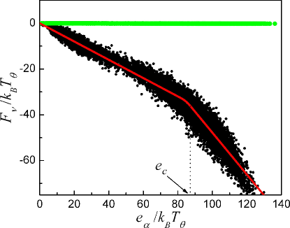
Figure 1: Vibrational free energies $F_{v}$ of inherent structures vs. their potential energies $e_{\alpha}$ (black points). The dependence is well-modeled by Eq. (4) with $e_{c}=88.4k_{B}T_{\theta}$ (piecewise-linear red line). The contribution from the highest 1/3 of the eigenvalues is constant (green points).

As demonstrated by the fit in Fig. 1, $F_{v}$ is well-modeled using the function

$$F_{v}(e_{\alpha})=k_{2}e_{\alpha} + (k_{2}-k_{1})k_{B}T_{\theta}$$ (4)

$$\times\ln\left(e^{-e_{c}/k_{B}T_{\theta}}+e^{-e_{\alpha}/k_{B}T_{\theta}}\right).$$

Equation (4) is essentially a piecewise-linear function with slope $k_{1}$ for $e_{\alpha}<e_{c}$, and slope $k_{2}$ for $e_{\alpha}>e_{c}$. For GB1, $k_{1}=-0.40$, $k_{2}=-0.91$, and $e_{c}=88.4k_{B}T_{\theta}$.

Inherent structure theory Stillinger and Weber (1982, 1984) assumes that $F_{v}(\alpha,T)=F_{v}(e_{\alpha},T)$ (validated for the present application in Fig. 1), and relates the vibrational free energy $F_{v}(e_{\alpha})$ and the probability distribution $P_{IS}(e_{\alpha})$ to the density of states $\Omega_{IS}(e_{\alpha})$ through

$$P_{IS}(e_{\alpha},T)={1\over Z}\Omega_{IS}(e_{\alpha})e^{-e_{\alpha}/k_{B}T}e^{-F_{v}(e_{\alpha},T)/k_{B}T}.$$ (5)

Given $\Omega_{IS}(e_{0})=1$, $F_{v}(e_{0},T)=0$, and $e_{0}=0$, $\Omega_{IS}(e_{\alpha})$ is given by

$$\Omega_{IS}(e_{\alpha})=e^{e_{\alpha}/k_{B}T}e^{F_{v}(e_{\alpha},T)/k_{B}T}{P_{IS}(e_{\alpha},T)\over P_{IS}(e_{0},T)},$$ (6)

which generalizes a similar equation in Nakagawa & Peyrard Nakagawa and Peyrard (2006) to values of $F_{v}(e_{\alpha},T)$ that vary with $e_{\alpha}$.

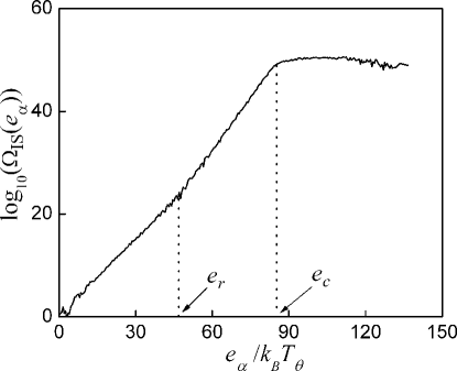
Figure 2: Density of inherent structures $\Omega_{IS}\left(e_{\alpha}\right)$. The knee at $e_{r}=47.4k_{B}T_{\theta}$ is due to a change in stress, and the plateau beginning at roughly $e_{c}=88.4k_{B}T_{\theta}$ is due to a change in rigidity; both are understood in terms of the network of native contacts (Figs. 3, 4).

We used Eq. (6) along with the calculated $P_{IS}(e_{\alpha})$ and $F_{v}(e_{\alpha})$ from Eq. (4) to model the density of inherent structures $\Omega_{IS}(e_{\alpha})$. At energies below $e_{c}$, $\Omega_{IS}(e_{\alpha})$ exhibits an exponential increase, but with a slight increase in the exponent factor above an energy $e_{r}$, giving rise to a knee in the plot of $\log\Omega_{IS}(e_{\alpha})$ vs. $e_{\alpha}$ (Fig. 2). The knee is located at a minimum in $P_{IS}(e_{\alpha})$ between the extended and collapsed states, and is thus associated with the transition state. Such a knee was also seen in a previous model of $\Omega_{IS}(e_{\alpha})$ that did not consider vibrations Nakagawa and Peyrard (2006). Above $e_{c}$, $\Omega_{IS}(e_{\alpha})$ plateaus and decreases at the highest energies, which is a consequence of the structure in both $P_{IS}(e_{\alpha})$ and $F_{v}(e_{\alpha},T_{\theta})$. Rather than being exponential in form Nakagawa and Peyrard (2006), from Eqs. [4] and [6], $\Omega_{IS}(e_{\alpha})$ in this region has the form

$$\Omega_{IS}(e_{\alpha})=e^{(1+k_{2})e_{\alpha}/k_{B}T}e^{(k_{1}-k_{2})e_{c}/k_{B}T_{\theta}}{P_{IS}(e_{\alpha},T)\over P_{IS}(e_{0},T)}.$$ (7)

Because $k_{2}$ is close to -1 at $T_{\theta}$, the structure of $\Omega_{IS}(e_{\alpha})$ closely resembles that of $P(e_{\alpha},T_{\theta})$ above $e_{c}$.

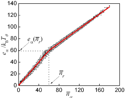
Figure 3: Potential energy $e_{\alpha}$ vs. number of broken contacts $\bar{n}_{\alpha}$. The dependence is well-modeled by Eq. (8) (red line). The energy required to break a native contact is approximately equal to the binding energy $\epsilon$, with differences due to stress in the structure. The knee corresponds to a change in stress at $\bar{n}_{r}=60$, where $e_{\alpha}(\bar{n}_{r})=59.6k_{B}T_{\theta}$.

We found (Fig. 3) that $e_{\alpha}$ is closely related to the number of broken native contacts, $\bar{n}_{\alpha}$ through the piecewise-linear function

$$e_{\alpha}=h_{2}\bar{n}_{\alpha}+(h_{2}-h_{1})\ln\left(e^{-\bar{n}_{r}}+e^{-\bar{n}_{\alpha}}\right).$$ (8)

The slopes $h_{1}$ and $h_{2}$ correspond to the amount of energy required to break a native contact below ($h_{1}$) and above ($h_{2}$) a critical number of broken contacts $\bar{n}_{r}$. Data for GB1 are well-modeled using $h_{1}=0.997$, $h_{2}=0.622$, and $\bar{n}_{r}=60$. Below $\bar{n}_{r}$, breaking a native contact requires more potential energy than above $\bar{n}_{r}$. Therefore, $\bar{n}_{r}$ is associated with a change in protein stress.

There are interesting connections between the structure of $\Omega_{IS}(e_{\alpha})$ below $e_{c}$ (Fig. 2) and the dependence of $e_{\alpha}$ on $\bar{n}_{\alpha}$ (Fig. 3). The change in the slope of $\Omega_{IS}$ at $e_{r}$ is closely related to the change in the slope of $e_{\alpha}(\bar{n}_{\alpha})$ at $\bar{n}_{r}$, suggesting that $\Omega_{IS}$ has a simple exponential dependence on $\bar{n}_{r}$ below $e_{c}$. However, the knee in $\Omega_{IS}$ occurs at $e_{r}=47.4k_{B}T_{\theta}$, which is smaller than the value $e_{\alpha}(\bar{n}_{r})=59.6k_{B}T_{\theta}$ at the knee in Fig. 3. While the density of inherent structures might truly be enhanced in the gap between $e_{r}$ and $e_{\alpha}(\bar{n}_{r})$, we note that the shift of $e_{r}$ with respect to $e_{\alpha}(\bar{n}_{r})$ might indicate that the inherent structure basins associated with the transition state are especially large (as noted above, $e_{r}$ is associated with the transition state), and that the harmonic approximation might be especially ill-suited to estimating their free energies for use in Eq. (6).

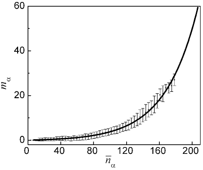
Figure 4: Number of residues $m_{\alpha}$ for which all native contacts are broken vs. the number of broken contacts $\bar{n}_{\alpha}$. The dependence is well-modeled by Eq. (9) (black line). Note that $m_{\alpha}=55$ (close to the expected value of 56) at $\bar{n}_{\alpha}=207$.

The source of the plateau in $\Omega_{IS}(e_{\alpha})$ above $e_{c}$ may be understood in terms of the dependence of the free energy on both $\bar{n}_{\alpha}$ and the number of residues $m_{\alpha}$ for which all native contacts are broken. As shown in Fig. 4, a plot of $m_{\alpha}$ vs. $\bar{n}_{\alpha}$ is well-modeled by the function

$$m_{\alpha}=\frac{1}{3}\left(e^{\bar{n}_{\alpha}/40}-1\right),$$ (9)

supporting an expectation that breaking a contact is only likely to create a residue with no native contacts at high $\bar{n}_{\alpha}$. The following simple model for $F_{v}$ then successfully captures the structure of $F_{v}$ in Fig. 1:

$$F_{v}(\bar{n}_{\alpha})=\nu\bar{n}_{\alpha}+\mu m_{\alpha},$$ (10)

with $m_{\alpha}$ given by Eq. (10). Using $\nu=-0.32$ and $\mu=-1.07$ yields good agreement between values of $F_{v}$ obtained either directly from the Hessian or using Eq. (10), with a correlation coefficient of 0.993 for values calculated from all inherent structures. We conclude that the change in the slope of $F_{v}$ vs. $e_{\alpha}$ at $e_{c}$, and therefore the plateau in $\Omega_{IS}(e_{\alpha})$ above $e_{c}$, is associated with an increase in the likelihood that breaking a native contact will increase the number of residues with no native contacts.

We found that protein stress and rigidity are closely tied to the network of native contacts through Eqs. [8] and [10]. This finding is remeniscent of an analysis of protein folding by Rader et al. Rader et al. (2002), in which the loss of network rigidity was associated with protein unfolding. It is therefore tempting to associate the region between $e_{r}$ and $e_{c}$ in Fig. 2 with the region of the mean coordination number $\left<r\right>$ where Rader et al. found that proteins become floppy and unfold. However, the present approach differs from that used by Rader et al. in two key ways. First, because all residue interactions in the present study are lumped into ${\rm C}_{\alpha}$ atoms, the coordination numbers are higher, and the relation of coordination numbers to protein rigidity might be different than for the all-atom models considered by Rader et al. Second, whereas the present results were obtained using a dynamical model, those obtained by Rader et al. were obtained using a static model of the protein. It will be interesting to further explore connections between the analyses based on IS theory and network rigidity; at present, they provide complementary perspectives on the relationship between protein dynamics and protein stress and rigidity.

The maximum in the density of states above $e_{c}$ is a consequence of considering diversity in vibrations, and is not observed when uniform vibrations are assumed Nakagawa and Peyrard (2006). Interestingly, a similar structure for the density of states, in which an exponential increase is followed by a maximum, has been observed for many structural-glass-forming liquids Stillinger and Weber (1984). It will therefore be interesting to improve the estimation of the density of states by obtaining more accurate estimates of $F_{v}$ than are possible using a harmonic approximation Baumketner et al. (2003).

Studies of two other G$\bar{\rm o}$ models of proteins yielded results that are similar to those found here for GB1 (unpublished results), suggesting the possibility that a simple phenomenological relationship between the network of native contacts and the energy landscape might exist for all G$\bar{\rm o}$ models. It will be interesting to explore this relationship for a large number of proteins and seek representations in which it is identical for different proteins. Discovery of such “universality” would enable the prediction of important properties of the energy landscapes of G$\bar{\rm o}$ models without performing numerical simulations.

It will be important to extend the present results to models whose energy landscapes exhibit more frustration than G$\bar{\rm o}$ models. For example, consider a modified model in which there is a weak attractive interaction for non-native contacts. In contrast to the simple relation illustrated in Fig. 3, in such a model, inherent structures with the same potential energy would likely have diverse numbers of native contacts. However, by extending the parameter space, the energy still might be simply related to a combination of both the number of native contacts and the number of non-native contacts. Similarly, the vibrational free energies might exhibit diversity among inherent structures with the same energy, but might still be simply related to both the number of native contacts and non-native contacts through an equation analogous to Eq. (10). Ultimately, it will be interesting to incrementally increase the complexity of the model, extending the present results (as far as computationally feasible) to realistic, all-atom models of proteins that include explicit solvent and other effects that are important in controlling protein function. Use of such all-atom models will enable the link between analyses based on IS theory and network rigidity to be further explored.

The present results demonstrate that simple connections to protein structure are hidden within the energy landscape of a G$\bar{\rm o}$ model. The potential energies and vibrational free energies of inherent structures are highly correlated, and both reflect simple measures of networks of native contacts. Through use of IS theory, these regularities should enable significant simplification of thermodynamic models of proteins Stillinger and Weber (1982, 1984); Nakagawa and Peyrard (2006).