The globular cluster system in NGC 5866: optical observations from HST Advanced Camera for Surveys

Abstract

We perform a detailed study of the Globular Cluster (GC) system in the galaxy NGC 5866 based on F435W, F555W, and F625W ($\sim$ B, V, and R) HST Advanced Camera for Surveys images.

Adopting color, size and shape selection criteria, the final list of GC candidates comprises 109 objects, with small estimated contamination from background galaxies, and foreground stars.

The color distribution of the final GC sample has a bimodal form. Adopting color to metallicity transformations derived from the Teramo–SPoT simple stellar population model, we estimate a metallicity [Fe/H]$\sim-1.5$, and $-$0.6 dex for the blue and red peaks, respectively. A similar result is found if the empirical color-metallicity relations derived from Galactic GCs data are used.

The two subpopulations show some of the features commonly observed in the GC system of other galaxies, like a “blue tilt”, higher central concentrations of the red subsystem, and larger half–light radii at larger galactocentric distances. However, we do not find evidence of a substantial difference between the average sizes of red and blue clusters.

Our analysis of the GC Luminosity Function indicates a V-band Turn-Over Magnitude V${}_{0}^{TOM}$=23.46$\pm$0.06, or M${}_{V,0}^{TOM}\sim-7.29\pm 0.10$ mag, using the distance modulus derived from the average of SBF and the PNLF distances. The absolute Turn-Over Magnitude obtained agrees well with calibrations from literature. The specific frequency is measured to be $S_{N}=1.4\pm 0.3$, typical for galaxies of this type.

1 Introduction

The study of the Globular Cluster (GC) system in galaxies is one of the fundamental keystones to understand the physical processes at the base of the formation and evolution of galaxies. The investigation of GC system properties involves aspects of several different fields in astronomy: stellar evolution, hierarchical assembly, the determination of extra–galactic distances, etc.

The first applications of the GCs as an investigation tool came in the earliest years of extra–galactic astronomy. Single bright GC were recognized as possible distance indicator in the 1950s (Baum, 1955), but it took few decades to develop the technique as it is applied now. The systematic study of the GC Luminosity Function (GCLF), in fact, has shown that it has a universal nearly gaussian shape. It is now recognized that the Turn Over Magnitude (TOM) of the GCLF is a reliable distance indicator for most galaxies, although some exceptions exist (Ferrarese et al., 2000; Richtler, 2003; Jordan et al., 2007).

Another, more recent discovery in the field of GC astronomy, is that the presence of a color bimodality is quite common in galaxies. The color bimodality has been mostly interpreted as a bimodal metallicity distribution (Harris, 2001; Brodie & Strader, 2006), leading to develop several possible GC formation scenarios, useful to constrain the history of galaxy formation. More recently, Kundu & Zepf (2007) using near-IR photometry, have shown that the GC bimodality in the giant ellipticals M 87 and NGC 4472 might represent true metallicity subpopulations. However, whether or not the bimodal color distribution is linked to the presence of two metallicity subpopulations is still a matter of debate, and there are claims that the optical properties of a bimodal GC system are not necessarily due to a bimodal metallicity distribution. For example, it has been shown that a bimodal color distributions might be generated by the combination of a unimodal metallicity distribution and a non-linear color-metallicity relation of the appropriate shape (Richtler, 2006; Yoon et al., 2006).

Furthermore, the advent of space-based astronomy has provided new information in this field. Most of all, the high resolution optical imaging of HST makes it possible to examine the shape properties, i.e. size and ellipticity, for an increasing number of extra–galactic GCs, up to distances as far as the Virgo Cluster (Jordan et al., 2007) and beyond. The examination of the characteristic sizes, and radial distribution of the blue and red GC subpopulations, enables the study of new phenomena related to the formation history of the GC system (Larsen & Brodie, 2003; Jordán, 2004).

In this paper we take advantage of archival HST images of the galaxy NGC 5866, taken with the Advanced Camera for Surveys (ACS) in the Wide Filed Camera mode, to carry out the first detailed multi-wavelength study of the GC system in this galaxy.

NGC 5866 is a lenticular galaxy, with a sharp dust lane nearly edge on. Being a disk galaxy, the GC system is expected to be less populated with respect to ellipticals (e.g. Harris & van den Bergh, 1981; Brodie & Strader, 2006). However, the quality of these ACS data allows us to analyze in some detail the clusters properties.

The weighted average of distances moduli obtained using the SBF (Tonry et al., 2001, using the new zeropoint from Jensen et al, 2003), and PNLF (Ciardullo et al., 2002) methods, provide a distance modulus $\mu_{0}=30.75\pm 0.08$, or 14.1$\pm$0.5 Mpc. At this distance, the GCs of the galaxy are near the ACS resolution limit, allowing us to carry out the size and shape analysis of the GC system.

The analysis of GC properties will be presented in the next sections. The observations and data reduction procedure are introduced in Section 2. Section 3 deals with the GC photometry and selection criteria. The color bimodality, color-magnitude relations, and the spatial distribution of the total GC system, as well as the two GC subpopulations, are discussed in Section 4. In the same Section we also make a comparison with stellar synthesis models. Finally, a study of GCLF and specific frequency is also presented in Section 4. We summarize and conclude the paper in Section 5.

2 Data reduction

The ACS/WFC camera observations of NGC 5866 were taken in February 2006 with the F435W, F555W and F625W filters ($\sim$ B, V, and R). The total exposure times for the three different passbands were: 3900s, 2800s and 2200s, respectively.

Standard reduction was carried out on raw images using the APSIS image processing software (Blakeslee et al., 2003). After cosmic–ray rejection, alignment, “drizzling”, and final image combination, we adopted an iterative procedure to determine the sky background and the galaxy best fit models, independently for the three passbands.

Since the galaxy fills the whole field of view of the ACS, the sky background determined in the outer corners of the CCD image is not accurate. We obtain the sky values extrapolating from the fit of a de Vaucouleurs $r^{1/4}$ profile.

Briefly, after masking out a few bright/saturated foreground stars, we adopt a provisional sky value from the corner with the lowest median number of counts. This value is subtracted to the image before starting the galaxy fitting procedure. Then, we fit the galaxy isophotes using the IRAF/STSDAS task ELLIPSE, which is based on the method described by Jedrzejewski (1987). Once the preliminary galaxy model is subtracted from the sky–subtracted frame, a wealth of faint sources appears together with the dust disk. A mask of these sources is obtained using a sigma detection method, and combined with the previous mask. The new mask is then fed to ELLIPSE to refit the galaxy’s isophotes.

After the geometric profile of the isophotes has been determined, we measure the galaxy flux in elliptical isophotes. At last, to improve the estimation of the sky, we fit the surface brightness profiles with a de Vaucouleurs $r^{1/4}$ profile plus a constant sky offset. The sky offset fitted is then adopted as the new sky value, and the whole procedure of galaxy fitting, source masking, surface brightness profile fitting and sky estimation is repeated, until convergence. This procedure is adopted for all three filters.

Once the sky and galaxy model have been subtracted from the frame, some large–scale deviations are still present in the frame. We remove these deviations using the background map obtained running SExtractor (Bertin & Arnouts, 1996) on the sky and galaxy subtracted frame. Part of the procedure adopted here is the same developed by Cantiello et al. (2005) to process ACS images for SBF analysis. We refer the reader to that paper for more details on the whole procedure of sky+galaxy+large scale residuals subtraction.

It is worth noting that in Cantiello et al. (2005) we have made some checks on the stability of the sky estimation against the fitting profile chosen. There, it was shown that, adopting a more general Sersic $r^{1/n}$ profile, the sky values obtained agree within uncertainties with those obtained adopting a de Vaucouleurs profile. In addition, in Cantiello et al. (2007), we compared the sky values obtained applying our method with the sky obtained by Sikkema et al. (2006) using a different approach, over a sample of 6 peculiar galaxies. As a result we found that the differences between the two sky background determinations is on average   $\sim$$<$ 3%.

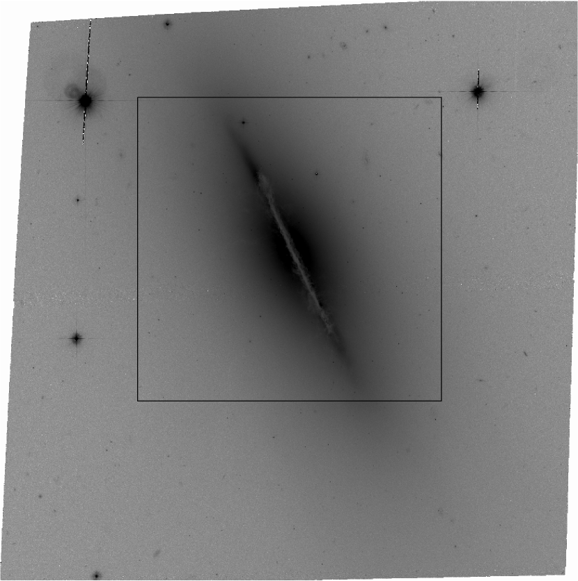
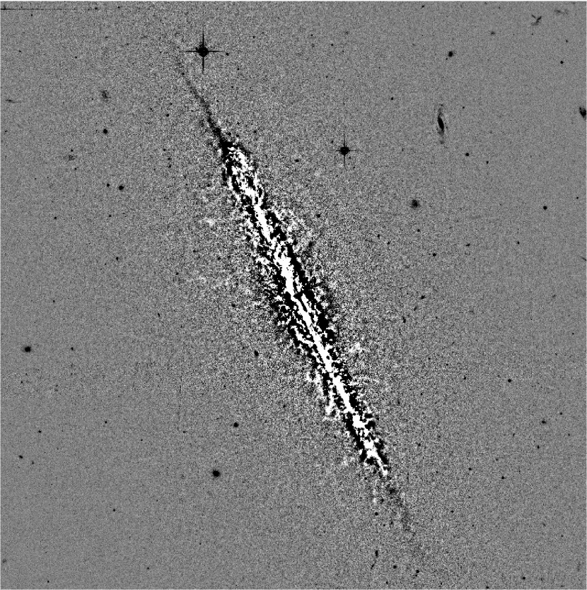
Figure 1: Left panel: NGC 5866 galaxy image from the HST ACS. The rectangle shows the location of area zoomed in the right panel. Right panel: A zoom of the disk of dust in NGC 5866 as seen in the residual frame.

Figure 1 shows the I-band ACS image of NGC 5866 (left panel), and a zoom of the sky+galaxy+large scale residuals subtracted frame (right panel, “residual” frame hereafter), the nearly edge–on dust disk in the galaxy is easily recognizable in this second panel.

3 Globular Cluster selection and photometry

The residual images were used for the detection and photometry of point-like and extended sources present in the frames. The source photometry was obtained independently on all three frames using SExtractor. After source detection, the output catalogs were matched using a 0.1^′′ radius.

To derive the aperture correction, standard growth curve analysis (Stetson, 1990) was performed on selected, isolated compact sources. Extinction corrections (values from Schlegel et al., 1998) and aperture corrections were applied before transforming the ACS magnitudes into the standard B, V and R magnitudes, using the prescriptions by Sirianni et al. (2005). The transformations from ACS to standard BVRI system magnitudes were obtained adopting the synthetic transformations from Sirianni et al. We have checked the compatibility of these magnitudes with the ones derived adopting the empirical transformations from Sirianni et al. As a result, we have found that the differences between the magnitudes obtained with the two set of transformations agree on average within 0.02 mag, at least in the range of colors of GC candidates which will be adopted later on.

We have chosen to select GC candidates using an approach similar to Spitler et al. (2006, S06 hereafter), based on the color, shape and size of the objects. At the distance of NGC 5866, the typical GC half-light radius, $r_{hl}\sim$3 pc, is at the limit of the angular resolution of the ACS camera (0.05 arcsec/pixel). Under such condition, the software ishape (Larsen, 1999) can be used to estimate the intrinsic shape parameters of slightly resolved objects. To run the $ishape$ software an oversampled PSF of the original image is needed. Based on their colors, we have selected a sample of star candidates from each frame and derived the PSF using the photometry package DAOPHOT, in the IRAF environment. The objects selected for PSF analysis were a posteriori confirmed to be stars.

In order to save computational time, we have removed from the initial catalog of matched sources all the sources easily recognizable as background galaxies. The new catalog was then fed to $ishape$, with the PSFs, to derive the shape parameters of the listed objects in the three different passbands. One of the main parameters to run $ishape$ is the convolution kernel, which, once convolved with the PSF, is used to fit the ellipticity, orientation, FWHM, etc. of the object. After various tests, we found that the best results were obtained adopting the analytic King profile, with concentration parameter c=30.

The final shape parameters for each object were then adopted as the average between the three estimations from the B, V and R frames. Those objects with half–light radius in one band more than 3–$\sigma$ different from the V-band $r_{hl}$ value, were rejected from the catalog. Similarly to S06, we have repeated such rejection procedure twice on the whole catalog of objects.

Next, we have rejected those object with $ishape$ ellipticities $\geq$ 0.5 ($<$ 10 objects at all). As a final selection criteria we have used the (B-R)₀ and (B-V)₀ color of the remaining sources. Only those objects whose color fell within the intervals 0.9$\leq(B-R)_{0}\leq$ 1.7, and $0.5\leq(B-V)_{0}\leq 1.1$ were taken as globular cluster candidates. After these selections, the final catalog of GC candidates consisted of 109 objects. The list of GC candidates, and their photometric, spatial and shape properties are reported in Table 1.

Before using these data, it is useful to estimate the amount of contamination from background galaxies and foreground stars.

Concerning the contamination due to background galaxies, given the similarity of NGC 5866 data with those of the Sombrero galaxy by S06, we adopt the conclusions from these authors. S06 have reduced and analyzed B and V images from Hubble Deep Field–North of the GOODS survey, and found that the number of background objects matching the GC selection criteria is $\sim$ 4% the final Sombrero GC sample. When this number is scaled to the imaging area of NGC 5866 ($\sim$1/6 of the Sombrero), and to the number of objects classified as GC, we find that in our case the contamination due to background galaxies is $\sim$ 6% the final number of GCs.

The number of galactic foreground stars expected in the color ranges adopted for GC selection have been calculated using the Bahcall & Soneira (1980) model. A number of approximately $\sim$ 8 stars is predicted to fall in the range of colors adopted for the GC selection. We find a similar, but somewhat lower number ($\sim$ 5-6 stars) using the models from Robin et al. (2003). These numbers have to be compared with the number of objects actually matching with the adopted color ranges, and rejected because of the small half-light radius, that is 4 objects at all. Given the small number statistics, we consider the number of contaminating stars from models consistent with the observed one, thus we can safely assume that the final sample of GC in Table 1 is likely free of contamination from foreground stars.

4 Discussion

4.1 Color histograms

Figure 2 shows the (B-R)₀, (B-V)₀ and (V-R)₀ color histograms for the 109 GC candidates. To test the bimodality of the color distribution of the GC sample we use the KMM code (McLachlan & Basford, 1988; Ashman et al., 1994). This code evaluates the likelihood whether or not the color distribution of sample is better represented by two gaussians or one single gaussian, the positions of the peaks are evaluated as well.

Running the KMM code on the (B-R)₀ color, returns a likelihood of $\sim$96% that the GC color distribution is bimodal, with peaks at (B-R)₀=1.12 (blue peak), and (B-R)₀=1.35 (red peak). The GCs are evenly assigned to each group.

An independent KMM run on the (B-V)₀ color, returned a slightly lower but significant bimodality probability (93 %), and peaks at (B-V)₀=0.67, (B-V)₀=0.84 mag.

The narrow range of GCs (V-R)₀ color, together with the small separation between the two possible peaks ($<0.1$ mag for the $\sim$ 600 GCs of the Sombrero galaxy), and the relatively small number of GC candidates, hampers any meaningful solution by KMM for this color.

At present, it is still a matter of debate what is the origin of the bimodality. The recent review from Brodie & Strader (2006) listed some of the different scenario proposed (major mergers, dissipationless accretion, hierarchical merging, etc.). In general the photometric data available, and the few spectroscopic measurements seem to point out that the primary difference between the two GC subpopulations is due to metallicity, without the need of invoking age variations. On the other hand, recently, it has been shown that a nonlinear color-metallicity relation could explain a bimodal color distribution without requiring a bimodal metallicity distribution (Richtler, 2006; Yoon et al., 2006).

If we assume the picture where the two color peaks are generated by a bimodal metallicity distribution, the metallicities corresponding to the peaks can be derived by assuming some [Fe/H] versus color relations. Adopting the view that GCs are mostly old, and using the Raimondo et al. (2005, R05 hereafter) models in the metallicity range $-1.8\leq$ [Fe/H] $\leq$ 0.3, for ages in the interval 9 $\leq$ t (Gyr) $\leq$ 14, we derive $[Fe/H]=(3.67\pm 0.13)(B-R)_{0}-(5.60\pm 0.18)$. We have verified the reliability of this equation by comparing the theoretical [Fe/H]_th. values predicted for the Galactic GCs, with the observational [Fe/H]_obs. estimations. For this comparison we have adopted the (B-R)₀ and [Fe/H]_obs. values from the updated online Harris (1996) catalog of Galactic GCs. As a result we find that the median difference is $\langle[Fe/H]_{th.}-[Fe/H]_{obs.}\rangle=-0.02\pm 0.16$ dex, confirming the reliability of the adopted color-metallicity relation. The good agreement of the models with Galactic GC data can also be seen in Figure 3 (left panel) where we show the fit of the [Fe/H] versus (B-R)₀ from the R05 models, and the Galactic GCs data.

Using the above [Fe/H] versus (B-R)₀ equation, the NGC 5866 peak metallicities are [Fe/H]=$-1.48\pm 0.23$, and $-$0.64$\pm$0.25 dex for the blue and red GC peaks, respectively.

We have repeated the above steps using (B-V)₀ colors instead of the (B-R)₀. The color-metallicity relation in this case is $[Fe/H]=(5.48\pm 0.19)(B-V)_{0}-(5.13\pm 0.16)$ (Fig. 3, right panel), which implies [Fe/H]=$-1.49\pm 0.20$, and $-0.54\pm 0.23$ dex for the two subpopulations.

These metallicity values can be considered quite average in bimodal GC systems. In fact, adopting the estimations for other galaxies reported by Brodie & Strader (2006), we find on average [Fe/H]=$-1.47\pm 0.12$ and $-0.48\pm 0.16$ dex for the sample of normal elliptical and S0 galaxies.

4.2 Blue tilt

Inspecting the color magnitude diagram of GCs, it has been shown that in some giant galaxies a color-luminosity correlation exists for the blue GCs (Harris et al., 2006). The interpretation of this correlation must be taken carefully, due to the limits of the GC selection criteria. Moreover, this phenomenon has not been detected in all galaxies (Mieske et al., 2006; Brodie & Strader, 2006)

To explain the existence of the color-luminosity correlation two different GC formation scenarios have been proposed: the self-enrichment, and the pre-enrichment one. The differences between these two scenarios is that in the first one the proto-GCs are able to trap and absorb the metals formed by stars within the GC; in the pre-enrichment scenario it is assumed that higher mass proto-GCs come from intrinsically higher metallicity clouds - see Strader et al. (2006) and references therein for more details.

Figure 4 shows the color magnitude diagrams for the NGC 5866 GCs. For the (B-R)₀ and (B-V)₀ we independently used the KMM output classification to separate the GC system into subpopulations. For the (V-R)₀ we used the combined results from the above colors to separate between the two subpopulations. It is worth noting that the sharp separation limits adopted to discriminate between the two sub-populations introduce a bias in the results, since real GC subsystems must overlap in some color range. Keeping in mind this warning, in Figure 4 we show the linear least–squares fits to the single subsystems.

We find a slight color-luminosity correlation for the blue GCs: the slope of the (B-R)₀ color versus R magnitude relation is $-0.012\pm 0.009$. The blue tilt is more evident if (B-V)₀ and (V-R)₀ data are taken into account, since with slopes $-0.017\pm 0.009$, and $-0.013\pm 0.003$, respectively. The slopes of the color-luminosity relations of the red sub-population are in all cases consistent with zero.

Using the color metallicity relations reported in the previous section to convert the tilt in terms of metallicity differences, we find that the brightest blue GC have on average $\sim$ 0.4 dex higher [Fe/H] respect to the faintest ones.

It is interesting to note that the study of a sample of bright ellipticals lead Harris et al. (2006) to conclude that color-luminosity relation appears more clearly in galaxies with larger number of clusters. An analogous result has been found by Mieske et al. (2006) by analyzing the GC properties for a sample of 79 Virgo Cluster galaxies. A similar conclusion can be drawn by comparing our data with the results of the Sombrero galaxy by S06. In fact, NGC 5866 is morphologically similar to the brighter Sombrero galaxy, but its GC population within $\sim$1.5 galactic effective radii is $\sim$ 1/5 the GC population in $\sim$1.5 effective radii of the Sombrero, and the (B-R)₀ versus R slope for blue GCs is almost one third the one derived from the Sombrero galaxy.

4.3 Spatial properties

One of the common results concerning the projected radial density of the GC subpopulations in galaxies, is that they can be fitted by a power law, with the red subpopulation being more centrally concentrated than the blue one. More specifically, it has been shown that the outer parts of GC systems are typically well-fit by power laws, while the central few kpc, hidden in these NGC 5866 data, often show the presence of cores (see, e.g., Ashman & Zepf, 1998).

Figure 5 shows the GC surface density in NGC 5866 versus the logarithm of galactocentric distance, $\log R_{gc}$. The upper panel shows the total density profile, while in the lower panel the profiles of the two GC subpopulations are shown separately. From this figure it is readily recognizable that $i$) the red subpopulation appears slightly more centrally concentrated respect to the blue one, $ii$) the density profiles are well fitted by power laws, with slopes: $-1.7\pm 0.3$, $-0.9\pm 0.3$, and $-1.3\pm 0.2$ for the red, blue, and total populations respectively. By comparing the slope of the total density profile with data from literature we find that NGC 5866 has an average behavior. In fact, using the compilation by Kissler-Patig (1997), we find that slopes in the range [$-$2.5,$-$1] are quite common in galaxies of total magnitude similar to NGC 5866, i.e., $M_{Bt}\sim-20$ mag.

The radial profiles of the (B-R)₀ color for the two subpopulations do not show significant radial gradients (upper panels in Figure 6). However, due to the different concentrations of the red and blue GCs shown in Figure 5, the total cluster population shows a clear color gradient (Figure 6, lower left panel). In the lower right panel of Figure 6 we show the (B-R)₀ color profile of the galaxy, the best fit line to the total GC color profile is shown, too. As can be recognized from this figure, the color profile of field stars closely resembles the color profile of the total GC system, with a $\sim+0.07$ mag shift, i.e. $\sim$ 0.3 dex higher metallicity.

These observational properties can be interpreted with a scenario where the metal poor blue GCs form in the early stages of the galaxy life, while the red GC component and the field stars are formed later on in a metal enriched potential well. Or, it could just be a metallicity gradient for both the GCs and field stars, combined with the nonlinear color-metallicity relation that originates the observed GC bimodal color distributions (Yoon et al., 2006; Richtler, 2006).

One other issue in understanding GC system formation and evolution, is the relation existing between the average sizes of GC subpopulations, and the variation of half-light radii with galactocentric distances.

Some observational data have shown that the half-light radii of the red subpopulation are on average 10% to 20% smaller than blue GC. Two different explanations have been given to this phenomenon. The one proposed by Larsen & Brodie (2003) involves a projection effect, due to the different spatial distribution of red and blue GCs, together with a strong correlation of the GC size with the galaxy radius. This model predicts that the size differences should be larger in the inner galactic regions, and disappear in the outskirts of the galaxy. In the other scenario, proposed by Jordán (2004), mass segregation and stellar evolution effects are the leading causes of the blue/red GC size differences. In this scenario little change of relative GC sizes with galactocentric distances is expected.

By comparing the average half-light radii of the red and blue GC in NGC 5866 we do not find any significant difference between the two subpopulations. Furthermore, the size versus galactocentric radius comparison, shown in Figure 7, reveals a slight tendency of outer GC to have larger half-light radii.

Due to the small number of GCs available, the absence of a clear size difference between the red and blue GCs, and the uncertainties in the half-light radius versus $R_{gc}$ correlation, these observations cannot be used to clearly support either the mass segregation or the projection scenarios.

4.4 Comparison with models

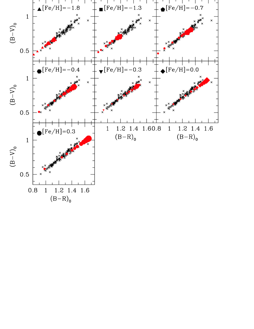
Figure 8: Observed GC colors compared with the R05 SSP models for ages $1\leq t(Gyr)\leq$ 14 and different metallicities (as labeled). [See electronic version of the Journal for a color version of the figure]

Figure 8 shows a comparison between the observed colors of NGC 5866 GCs and the predictions from R05. Each panel in the figure shows a Simple Stellar Population (SSP) model with a defined [Fe/H], and for ages 1 $\leq$ t (Gyr) $\leq$ 14.

At first glance, these panels will give little information about the age and metallicity properties of the observed GCs, due to the strong overlap of models with different physical properties. This is not related to the particular choice of SSP models. In order to reduce model systematics, we have also considered a data to models comparison using the Bruzual & Charlot (2003) SSP models. The new set of models essentially agrees with the R05 one, and the overlap between models at different [Fe/H] is still present. Moreover, since the R05 models are optimized to match in detail the observational features of Color Magnitude Diagrams of Galactic and Magellanic Clouds stellar clusters, in this section we will take the set of stellar synthesis models from R05 as reference ones.

If no constraint is put on models, the conclusions that can be drawn from the comparison shown in Figure 8 are mainly: $i$) SSP models, i.e. single age and single metallicity stellar systems, reproduce nicely the observational color-color properties of GCs; $ii$) except one single object, no old super metal-rich (t $>$ 7 Gyr, [Fe/H]$>$[Fe/H]_☉) GC seems to be present; $iii$) the reddest GCs in the sample [(B-R)${}_{0}\sim$1.6, (B-V)${}_{0}\sim$1] are either old, t$\sim$ 14 Gyr, solar metallicity objects, or younger, t$\sim$ 5 Gyr, super-solar metallicity stellar systems.

However, if we limit the models to the range of old age models (9 $\leq$ t (Gyr) $\leq$ 14) some stronger constraints on the age and metallicity of the GC can be obtained. To support this choice, as mentioned before, we recall that old GC ages have been found in most of the GC systems in galaxies both with photometric and spectroscopic data (Brodie & Strader, 2006). In addition to this, as shown in Figure 9 (upper panels), the range of (B-R)₀ and (B-V)₀ colors for NGC 5866 and for Galactic GCs appears to be very similar. If we assume that such color similarity is also associated with common physical characteristics of the GC systems, than we can adopt for NGC 5866 an age range similar to the one of Galactic GC, that is 9   $\sim$$<$  t (Gyr)   $\sim$$<$  14 (e.g. De Angeli et al., 2005).

Based on these considerations, we can go back to the comparisons shown in Figure 8, taking into account only the models in the selected age interval. With this constraint we find that the blue tail of GCs has [Fe/H]$\leq-1.8$ dex. If we extrapolate the [Fe/H] versus (B-R)₀ equation derived from R05 models using the same age limitations adopted here, then the most metal poor GC in NGC 5866 has [Fe/H]$\sim-2.3$ dex. On the other hand, inspecting the color properties of red clusters, the conclusion is that the reddest GCs in NGC 5866 are old objects, t$\sim$14 Gyr, with nearly solar metallicity.

Before concluding this section, we find interesting to note that if the same arguments are applied to the GC system in the Sombrero galaxy (data from S06, shown in the right panels of Figure 9), the metallicity range spanned by the GC system is $-2.2\ \raise-2.0pt\hbox{\hbox to0.0pt{\hbox{$\sim$}\hss}\raise 5.0pt\hbox{$<$}\ }$ [Fe/H]   $\sim$$<$  0.6. Thus, while the blue tails of the GC system appear to be quite similar in the three galaxies, the red tail of the GCs in the Sombrero includes also a population of very metal rich clusters.

4.5 Globular Cluster Luminosity Function

The review by Richtler (2003) gives a fairly detailed study on the use of GCs as distance indicators. By comparing GCLF distances with those derived using the SBF method, Richtler proves that the TOM is a good distance indicator, although some exceptions exists, related to a possible contamination from intermediate age GCs, or young massive clusters.

Figure 10 shows the V-band completeness functions for NGC 5866 derived within three annular regions with radii $R_{gc}(arcsec)\leq 35$, $35<R_{gc}(arcsec)\leq 70$, and $R_{gc}(arcsec)>70$. A 95% completeness level is reached at V${}_{0}=23.9,~{}24.8,~{}25.1$ mag for the three different annuli, respectively. The completeness functions have been derived via standard artificial star tests, using the DAOPHOT task $addstar$ to generate the artificial stars, then we ran SExtractor for the detection of sources, as described in Section 2.

Adopting SBF distances, Richtler (2003) obtained an absolute TOM M${}_{V,0}=-7.35\pm 0.25$ mag, which at the distance of NGC 5866 translates into an apparent TOM V${}_{0}^{TOM}\sim$ 23.46 mag. This means that the GCLF is fairly complete up to $\sim$0.5, 1.4, and 1.7 magnitudes fainter than the TOM in the three different annular regions taken into account.

Fitting a gaussian distribution to the GCLF corrected for incompleteness, gives a TOM V${}_{0}^{TOM}=23.46\pm 0.06$ mag, with a dispersion $\sigma=1.13\pm 0.05$. Adopting the SBF+PNLF average distance $\mu_{0}=30.75\pm 0.08$, the absolute TOM is M${}_{V,0}^{TOM}=-7.29\pm 0.10$ mag, in nice agreement with the value provided by Richtler.

4.6 Specific Frequency

Although the field of view of the ACS camera does not sample the whole NGC 5866 area, we have obtained an estimation for the Specific frequency, $S_{N}$, of GCs over the ACS sampling area.

The concept of specific frequency, $S_{N}=N_{GC}\times 10^{0.4(M_{V}+15)}$, was introduced by Harris & van den Bergh (1981) as a tool to quantify the amount of stars in GCs with respect to the amount of field stars in a galaxy. To derive $S_{N}$ we choose to not do any extrapolation to derive the total $N_{GC}$ and the total magnitude, $m_{V}$, to avoid the uncertainty introduced by the profile extrapolation. Instead, adopting an approach similar to Blakeslee et al. (1997), we adopt the number of GCs found in the ACS sampling area, after completeness correction, and the total magnitude obtained from the same masked frame that we used to detect GCs ($m_{V}=10.9\pm 0.1$ mag).

As noted by Blakeslee et al. (1997), if the GC system follows the same radial profile of the galaxy light in the outer regions, there should be little difference between the global $S_{N}$ and this $S_{N}$ over a limited area, referred to as “metric $S_{N}$” by Blakeslee et al.

With these assumptions, we derive $S_{N}=1.4\pm 0.3$, which is within the normal $S_{N}$ range for galaxies in the same luminosity class of NGC 5866 ($S_{N}$=0.7-7.5, Kissler-Patig, 1997). We have also estimated the total $S_{N}$ extrapolating the total number of GCs. By integrating over the surface density, corrected for magnitude completeness, we obtained $N_{GC}^{Total}\sim 400$. Adopting a total magnitude $m_{V}\sim 9.8\pm 0.1$ mag from the RC3 catalog, we find $S_{N}^{Total}\sim 1.6\pm 0.4$, in nice agreement with the value found over the limited ACS area.

Finally, since the GCs are evenly distributed between the two subpopulations, we find that the specific frequency for the blue and red subsystems is $S_{N}^{blue}\sim S_{N}^{red}\sim 0.7$.

5 Conclusions

We have used archival HST data to study the GC system of NGC 5866 galaxy in the B, V and R passbands. Using standard color, size and shape selection criteria, the final list of GC candidates consists of 109 objects. The estimated contamination from background galaxies is $\sim$ 6 % of the sample, while essentially no contamination is expected from foreground stars.

The color distribution of the GC system has a bimodal form. Adopting the color-metallicity relations from R05 models, we find that the blue and red peaks correspond to a metallicity [Fe/H]$\sim-1.5$, and $-$0.6 dex, respectively. These metallicity peaks are quite average among the galaxies with known color bimodality. Similarly, we have found that the specific frequency of GCs is $S_{N}=1.4\pm 0.3$, which is a normal value for galaxies of the same luminosity class of NGC 5866.

By inspecting the color magnitude diagram of the two GC subsystems, a color-luminosity correlation appears in the blue GCs, with brighter objects being slightly redder than the fainter ones. Interpreting this feature as a luminosity-metallicity correlation, the bright blue GCs are found to be 0.4 dex more metal rich than the fainter ones.

Inspecting the spatial properties of the GCs, we find that $i$) the red subpopulation appears to be more centrally concentrated than the blue one; $ii$) the radial density of the total GC population, and of the two subpopulations taken separately, follows a power law radial profile; and that $iii$) the GCs have larger half-light radii at larger galactocentric distances. We do not find any sign of a significant difference between the average sizes of the subpopulations.

Taken separately, the two GC subsystems do not show significant color gradients. However, due to the different radial concentrations, the total GC system shows a color gradient, very similar to the one of field stars, except that the GCs are systematically $\sim$0.1 mag bluer in (B-R)₀. If the GC to field stars color offset is simply associated to a metallicity difference, then the population of field stars at a given galactocentric distance is, on average, 0.3 dex more metal rich of the GC population at the same radius.

A comparison of data with the R05 models has shown that no old, very metal rich (t$>$9 Gyr, [Fe/H]$>$0) cluster is present. Moreover, if only models in the age range 9$\leq$ t (Gyr) $\leq$ 14 are taken into account, then the metallicity range for the GC system in this galaxy is found to be $-2.3\lesssim$ [Fe/H] $\lesssim 0.0$. When compared to Galactic and Sombrero data, we find that NGC 5866 and Milky Way GC share similar metallicity range, while the Sombrero has a tail of very metal rich GCs ([Fe/H] $\sim 0.6$).

The study of the GC luminosity function has shown that the GC sample is fairly complete out to $\sim$1.2 mag below the expected TOM. A gaussian fit to the GCLF provided us V${}_{0}^{TOM}=23.46\pm 0.06$ mag. Adopting a distance modulus $\mu_{0}=30.75\pm 0.08$ from the weighted average of SBF and PNLF distances, implies M${}_{V,0}^{TOM}=-7.29\pm 0.10$ mag, in agreement with the mean value from Richtler (2003).

Figure 2: Color histograms of the final sample of GC candidates.

Figure 3: Left panel: Galactic GC (B-R)₀ color and [Fe/H] data (full dots) compared with the linear fit to the R05 models (dotted line, see text). The fit to the models nicely agrees with observational data. Right panel: as left panel, but for (B-V)₀ color.

Figure 4: Color-Magnitude Diagrams of the final sample of GC. There is some evidence of the color-magnitude tilt for the blue GC subpopulation (empty squares). No significant tilt is found in the red peak GC candidates (full squares). The dashed lines show the least-squares fit to the data.

Figure 5: Upper panel: The surface density of the entire GC population. The least-squares profile fit (solid line) shows that the radial density profile is well reproduced by a power law, $\log\sigma_{GC}=(-1.3\pm 0.1)\log R_{gc}+(1.0\pm 0.1)$. Lower panel: Same as upper panel but the two subpopulations are shown separately. The dotted (dashed) line represents a linear fit to the data of red (blue) GCs. The fitted lines show that the red subpopulation is more centrally concentrated than the blue one.

Figure 6: GC colors versus the galactocentric distance. The crosses mark actual GC data. Full big squares correspond to a running average of data, error bars are shown with small squares. The upper two panels show that no significant radial color gradient exists if the two subpopulations are taken separately into account. If the whole GC system is considered, a non negligible color gradient is found, with bluer GC colors in the galaxy outskirts (down left panel). The galaxy color profile (thick solid line, uncertainties shown with thin lines), and the least-squares line of the GC system radial profile (dashed line) are shown in the lower right panel.

Figure 7: Cluster sizes versus the galactocentric distance. The dashed lines show the least-squares fit to the data. These data show the tendency of larger GC radii at larger galactocentric distances.

Figure 9: Color-color comparisons (upper panels), and (B-R)₀ color histograms (lower panels) for Galactic, NGC 5866 and Sombrero clusters, as labeled. The least-squares fit lines are also shown. The Sombrero GC system includes a rich component of red, super metal rich globular clusters which is practically missing in the other two galaxies system. On the other hand, the blue tails of the GC distributions are quite similar for the three galaxies.

Figure 10: V-band completeness functions within three different galactocentric annuli.

Figure 11: The observed GCLF histogram (corrected for incompleteness) and the best fit gaussian line. The TOM obtained is V${}_{0}^{TOM}=23.46\pm 0.06$ mag (dashed line), dispersion $\sigma=1.13\pm 0.05$. Adopting such TOM magnitude we derive the absolute TOM $M_{V,0}^{TOM}=-7.29\pm 0.10$ mag, in agreement with the “universal” value from Richtler (2003). The 95% completentess magnitude limits at different galactic annuli are also shown in the figure with vertical arrows.

Table 1: Globular Clusters in NGC 5866

R.A.	Decl.	Rgc	B0	V0	R0	(B-R)0	(B-V)0	(V-R)0	rhl	[Fe/H]
(J2000)	(J2000)	arcsec	mag	mag	mag	mag	mag	mag	pc	dex
15 06 20.43	55 46 11.78	12.34	24.19 $\pm$ 0.03	23.57 $\pm$ 0.03	23.13 $\pm$ 0.02	1.05	0.62	0.43	2.16	-1.73 $\pm$ 0.20
15 06 21.23	55 46 21.65	16.31	23.38 $\pm$ 0.03	22.78 $\pm$ 0.02	22.33 $\pm$ 0.02	1.05	0.60	0.46	1.89	-1.79 $\pm$ 0.18
15 06 20.06	55 45 01.26	16.97	25.00 $\pm$ 0.04	24.16 $\pm$ 0.03	23.65 $\pm$ 0.02	1.35	0.84	0.51	4.30	-0.60 $\pm$ 0.22
15 06 22.81	55 47 01.20	19.21	23.50 $\pm$ 0.03	22.71 $\pm$ 0.02	22.20 $\pm$ 0.02	1.30	0.80	0.51	2.23	-0.79 $\pm$ 0.20
15 06 23.30	55 46 57.11	19.98	22.57 $\pm$ 0.02	21.85 $\pm$ 0.02	21.34 $\pm$ 0.01	1.23	0.71	0.51	4.27	-1.15 $\pm$ 0.18
15 06 22.41	55 45 59.70	20.02	24.78 $\pm$ 0.04	24.19 $\pm$ 0.03	23.75 $\pm$ 0.03	1.03	0.59	0.44	2.02	-1.87 $\pm$ 0.22
15 06 23.15	55 46 09.52	20.14	24.40 $\pm$ 0.04	23.54 $\pm$ 0.03	23.04 $\pm$ 0.03	1.36	0.85	0.50	2.36	-0.54 $\pm$ 0.23
15 06 23.84	55 46 30.53	21.34	25.18 $\pm$ 0.06	24.54 $\pm$ 0.05	24.07 $\pm$ 0.05	1.11	0.64	0.47	3.59	-1.56 $\pm$ 0.28
15 06 22.32	55 45 03.33	22.61	22.77 $\pm$ 0.02	22.15 $\pm$ 0.02	21.72 $\pm$ 0.01	1.05	0.62	0.43	2.61	-1.73 $\pm$ 0.18
15 06 23.97	55 46 04.64	23.20	23.66 $\pm$ 0.03	23.03 $\pm$ 0.03	22.58 $\pm$ 0.02	1.08	0.63	0.45	2.04	-1.64 $\pm$ 0.20
15 06 23.84	55 45 49.92	23.44	24.00 $\pm$ 0.03	23.08 $\pm$ 0.02	22.56 $\pm$ 0.02	1.44	0.91	0.53	1.79	-0.23 $\pm$ 0.22
15 06 23.34	55 45 06.89	26.21	23.02 $\pm$ 0.02	22.37 $\pm$ 0.02	21.91 $\pm$ 0.01	1.10	0.65	0.45	2.95	-1.55 $\pm$ 0.18
15 06 24.73	55 46 06.46	26.29	25.30 $\pm$ 0.08	24.43 $\pm$ 0.06	23.95 $\pm$ 0.05	1.35	0.86	0.48	3.63	-0.56 $\pm$ 0.34
15 06 23.02	55 44 35.84	26.74	24.28 $\pm$ 0.03	23.66 $\pm$ 0.02	23.19 $\pm$ 0.02	1.08	0.62	0.47	2.35	-1.68 $\pm$ 0.19
15 06 25.16	55 46 06.95	26.83	24.79 $\pm$ 0.06	24.12 $\pm$ 0.05	23.63 $\pm$ 0.05	1.15	0.67	0.49	2.62	-1.41 $\pm$ 0.28
15 06 26.45	55 47 04.16	28.46	23.40 $\pm$ 0.02	22.75 $\pm$ 0.02	22.29 $\pm$ 0.02	1.12	0.66	0.46	2.89	-1.51 $\pm$ 0.18
15 06 25.51	55 46 09.26	28.97	24.93 $\pm$ 0.07	24.14 $\pm$ 0.06	23.62 $\pm$ 0.05	1.31	0.79	0.53	5.77	-0.80 $\pm$ 0.33
15 06 25.09	55 45 45.82	30.28	25.36 $\pm$ 0.06	24.75 $\pm$ 0.05	24.41 $\pm$ 0.06	0.95	0.61	0.34	3.23	-1.99 $\pm$ 0.30
15 06 25.95	55 46 21.25	30.43	25.32 $\pm$ 0.07	24.48 $\pm$ 0.05	23.89 $\pm$ 0.05	1.42	0.84	0.59	4.90	-0.44 $\pm$ 0.33
15 06 24.71	55 45 23.59	31.73	24.86 $\pm$ 0.04	24.35 $\pm$ 0.03	23.93 $\pm$ 0.03	0.92	0.51	0.42	3.82	-2.27 $\pm$ 0.22
15 06 27.61	55 47 23.81	32.72	24.16 $\pm$ 0.03	23.30 $\pm$ 0.02	22.77 $\pm$ 0.02	1.39	0.86	0.53	2.63	-0.47 $\pm$ 0.21
15 06 26.05	55 46 01.35	32.80	22.94 $\pm$ 0.03	22.14 $\pm$ 0.02	21.61 $\pm$ 0.02	1.33	0.80	0.53	3.27	-0.72 $\pm$ 0.21
15 06 24.40	55 44 37.65	34.98	23.76 $\pm$ 0.03	23.14 $\pm$ 0.02	22.68 $\pm$ 0.02	1.08	0.63	0.45	3.11	-1.66 $\pm$ 0.19
15 06 26.79	55 46 17.51	35.00	23.50 $\pm$ 0.03	22.83 $\pm$ 0.03	22.37 $\pm$ 0.03	1.13	0.67	0.46	3.41	-1.45 $\pm$ 0.21
15 06 28.11	55 47 20.25	35.27	25.34 $\pm$ 0.05	24.50 $\pm$ 0.03	24.01 $\pm$ 0.03	1.33	0.84	0.49	5.32	-0.64 $\pm$ 0.25
15 06 25.97	55 45 46.75	35.27	24.93 $\pm$ 0.06	23.98 $\pm$ 0.04	23.46 $\pm$ 0.04	1.47	0.94	0.53	5.67	-0.12 $\pm$ 0.28
15 06 25.72	55 45 21.38	36.12	22.82 $\pm$ 0.02	22.14 $\pm$ 0.02	21.68 $\pm$ 0.02	1.14	0.68	0.46	2.06	-1.41 $\pm$ 0.18
15 06 26.25	55 45 42.93	37.89	24.61 $\pm$ 0.05	23.77 $\pm$ 0.04	23.21 $\pm$ 0.03	1.40	0.84	0.56	2.02	-0.49 $\pm$ 0.25
15 06 26.96	55 46 16.29	37.94	24.32 $\pm$ 0.05	23.58 $\pm$ 0.04	23.03 $\pm$ 0.03	1.29	0.74	0.55	5.73	-0.95 $\pm$ 0.25
15 06 26.02	55 46 18.00	38.51	22.95 $\pm$ 0.03	22.35 $\pm$ 0.02	21.92 $\pm$ 0.02	1.04	0.60	0.44	2.60	-1.81 $\pm$ 0.19
15 06 26.51	55 45 52.59	38.87	22.68 $\pm$ 0.03	21.87 $\pm$ 0.02	21.36 $\pm$ 0.02	1.31	0.81	0.51	2.50	-0.74 $\pm$ 0.20
15 06 25.81	55 45 17.43	40.51	24.24 $\pm$ 0.03	23.59 $\pm$ 0.03	23.15 $\pm$ 0.02	1.09	0.65	0.45	2.63	-1.59 $\pm$ 0.20
15 06 27.12	55 46 15.90	41.83	24.16 $\pm$ 0.04	23.28 $\pm$ 0.03	22.76 $\pm$ 0.03	1.40	0.87	0.52	2.21	-0.41 $\pm$ 0.24
15 06 27.78	55 46 26.76	41.89	23.07 $\pm$ 0.03	22.12 $\pm$ 0.02	21.59 $\pm$ 0.02	1.48	0.95	0.53	2.82	-0.03 $\pm$ 0.21
15 06 27.84	55 46 15.80	41.97	25.61 $\pm$ 0.10	24.71 $\pm$ 0.07	24.10 $\pm$ 0.06	1.50	0.90	0.61	4.98	-0.13 $\pm$ 0.41
15 06 26.59	55 45 05.26	42.54	22.30 $\pm$ 0.02	21.61 $\pm$ 0.02	21.15 $\pm$ 0.01	1.15	0.69	0.46	2.30	-1.36 $\pm$ 0.18
15 06 28.82	55 46 50.49	42.61	25.57 $\pm$ 0.06	24.55 $\pm$ 0.04	24.09 $\pm$ 0.03	1.48	1.02	0.46	2.42	0.08 $\pm$ 0.28
15 06 27.64	55 45 46.80	42.66	22.18 $\pm$ 0.03	21.42 $\pm$ 0.02	20.91 $\pm$ 0.02	1.27	0.76	0.52	1.99	-0.95 $\pm$ 0.20
15 06 28.45	55 46 25.36	42.86	24.10 $\pm$ 0.03	23.47 $\pm$ 0.03	23.02 $\pm$ 0.03	1.08	0.63	0.45	3.40	-1.65 $\pm$ 0.20
15 06 28.71	55 46 35.43	43.84	23.98 $\pm$ 0.03	23.26 $\pm$ 0.02	22.80 $\pm$ 0.02	1.18	0.72	0.46	2.97	-1.24 $\pm$ 0.20
15 06 26.69	55 44 44.60	44.97	22.17 $\pm$ 0.02	21.50 $\pm$ 0.02	21.05 $\pm$ 0.01	1.13	0.67	0.45	3.19	-1.46 $\pm$ 0.18
15 06 27.85	55 45 35.12	45.04	22.90 $\pm$ 0.03	22.12 $\pm$ 0.02	21.65 $\pm$ 0.02	1.25	0.78	0.47	2.21	-0.95 $\pm$ 0.20
15 06 27.46	55 45 09.04	45.43	23.60 $\pm$ 0.03	23.02 $\pm$ 0.02	22.58 $\pm$ 0.02	1.02	0.58	0.44	3.08	-1.92 $\pm$ 0.18
15 06 27.97	55 45 33.02	46.01	23.94 $\pm$ 0.04	23.00 $\pm$ 0.03	22.49 $\pm$ 0.03	1.45	0.94	0.51	2.02	-0.15 $\pm$ 0.24
15 06 26.83	55 44 25.46	47.61	23.47 $\pm$ 0.03	22.68 $\pm$ 0.02	22.20 $\pm$ 0.02	1.27	0.79	0.48	2.93	-0.87 $\pm$ 0.19
15 06 29.35	55 46 22.64	48.30	23.47 $\pm$ 0.03	22.74 $\pm$ 0.02	22.27 $\pm$ 0.02	1.20	0.73	0.47	2.71	-1.15 $\pm$ 0.19
15 06 29.46	55 46 11.11	48.43	24.20 $\pm$ 0.04	23.42 $\pm$ 0.03	22.93 $\pm$ 0.03	1.27	0.78	0.49	2.96	-0.91 $\pm$ 0.23
15 06 29.03	55 45 24.94	48.95	23.54 $\pm$ 0.03	22.87 $\pm$ 0.03	22.40 $\pm$ 0.02	1.14	0.66	0.48	3.24	-1.45 $\pm$ 0.20
15 06 30.53	55 46 32.97	49.34	24.70 $\pm$ 0.04	24.01 $\pm$ 0.03	23.54 $\pm$ 0.03	1.17	0.70	0.47	2.71	-1.31 $\pm$ 0.22
15 06 29.94	55 45 59.62	50.20	21.84 $\pm$ 0.03	20.96 $\pm$ 0.02	20.44 $\pm$ 0.02	1.40	0.88	0.52	2.29	-0.40 $\pm$ 0.21
15 06 31.60	55 47 08.10	50.70	25.01 $\pm$ 0.04	24.38 $\pm$ 0.03	24.02 $\pm$ 0.03	0.99	0.63	0.36	2.60	-1.85 $\pm$ 0.21
15 06 29.61	55 45 27.53	51.80	23.03 $\pm$ 0.03	22.22 $\pm$ 0.03	21.65 $\pm$ 0.02	1.38	0.81	0.57	1.99	-0.59 $\pm$ 0.21
15 06 30.61	55 46 08.54	52.50	25.13 $\pm$ 0.07	24.46 $\pm$ 0.05	24.01 $\pm$ 0.05	1.12	0.67	0.45	2.12	-1.48 $\pm$ 0.30
15 06 31.71	55 46 55.76	53.60	23.42 $\pm$ 0.02	22.87 $\pm$ 0.02	22.42 $\pm$ 0.02	1.00	0.55	0.44	4.49	-2.01 $\pm$ 0.17
15 06 29.24	55 44 55.99	55.55	24.74 $\pm$ 0.04	23.92 $\pm$ 0.03	23.42 $\pm$ 0.03	1.31	0.81	0.50	2.02	-0.74 $\pm$ 0.23
15 06 30.34	55 45 21.76	56.10	24.01 $\pm$ 0.05	23.17 $\pm$ 0.04	22.67 $\pm$ 0.04	1.34	0.84	0.50	2.02	-0.63 $\pm$ 0.27
15 06 30.41	55 45 18.26	56.60	24.23 $\pm$ 0.06	23.46 $\pm$ 0.04	23.02 $\pm$ 0.04	1.21	0.77	0.43	1.96	-1.07 $\pm$ 0.28
15 06 31.41	55 45 54.54	57.10	23.67 $\pm$ 0.05	22.80 $\pm$ 0.04	22.31 $\pm$ 0.04	1.35	0.86	0.49	2.33	-0.54 $\pm$ 0.27
15 06 31.75	55 45 58.62	57.75	24.17 $\pm$ 0.05	23.56 $\pm$ 0.04	23.08 $\pm$ 0.04	1.09	0.61	0.48	2.77	-1.65 $\pm$ 0.26
15 06 31.15	55 45 21.98	58.45	23.98 $\pm$ 0.04	23.29 $\pm$ 0.03	22.82 $\pm$ 0.03	1.16	0.68	0.47	1.65	-1.37 $\pm$ 0.23
15 06 31.43	55 45 25.88	58.45	23.28 $\pm$ 0.04	22.42 $\pm$ 0.03	21.93 $\pm$ 0.03	1.34	0.85	0.49	1.97	-0.58 $\pm$ 0.22
15 06 31.95	55 45 46.99	61.60	23.93 $\pm$ 0.04	23.13 $\pm$ 0.04	22.62 $\pm$ 0.03	1.31	0.80	0.52	2.74	-0.77 $\pm$ 0.25
15 06 31.04	55 44 55.54	63.15	24.18 $\pm$ 0.04	23.42 $\pm$ 0.03	22.95 $\pm$ 0.02	1.23	0.76	0.47	2.44	-1.03 $\pm$ 0.22
15 06 30.85	55 44 43.28	63.30	23.64 $\pm$ 0.03	23.00 $\pm$ 0.02	22.55 $\pm$ 0.02	1.10	0.64	0.46	2.63	-1.60 $\pm$ 0.19
15 06 32.99	55 46 19.41	64.35	23.78 $\pm$ 0.03	23.10 $\pm$ 0.02	22.63 $\pm$ 0.02	1.15	0.69	0.46	2.40	-1.38 $\pm$ 0.19
15 06 32.54	55 45 55.30	64.60	21.58 $\pm$ 0.02	20.86 $\pm$ 0.02	20.38 $\pm$ 0.01	1.20	0.72	0.48	3.02	-1.19 $\pm$ 0.18
15 06 30.42	55 44 11.48	65.30	26.14 $\pm$ 0.08	25.39 $\pm$ 0.06	24.97 $\pm$ 0.05	1.17	0.76	0.41	4.71	-1.20 $\pm$ 0.34
15 06 32.90	55 46 04.62	66.30	25.52 $\pm$ 0.07	24.75 $\pm$ 0.05	24.24 $\pm$ 0.05	1.28	0.77	0.51	7.83	-0.92 $\pm$ 0.30
15 06 31.47	55 44 53.38	66.55	24.66 $\pm$ 0.04	24.08 $\pm$ 0.03	23.67 $\pm$ 0.03	1.00	0.58	0.42	2.54	-1.94 $\pm$ 0.21
15 06 32.27	55 45 20.77	67.05	24.18 $\pm$ 0.05	23.41 $\pm$ 0.04	22.92 $\pm$ 0.03	1.26	0.76	0.50	5.66	-0.97 $\pm$ 0.25
15 06 32.27	55 45 20.77	67.60	24.18 $\pm$ 0.05	23.34 $\pm$ 0.04	22.84 $\pm$ 0.03	1.33	0.83	0.50	5.66	-0.65 $\pm$ 0.25
15 06 32.60	55 45 10.58	70.45	23.82 $\pm$ 0.04	23.06 $\pm$ 0.03	22.53 $\pm$ 0.03	1.29	0.76	0.52	2.94	-0.91 $\pm$ 0.22
15 06 32.96	55 45 21.88	70.70	24.54 $\pm$ 0.06	23.62 $\pm$ 0.04	23.10 $\pm$ 0.04	1.44	0.92	0.52	2.10	-0.22 $\pm$ 0.28
15 06 32.67	55 45 04.23	71.05	23.60 $\pm$ 0.03	22.71 $\pm$ 0.02	22.20 $\pm$ 0.02	1.40	0.89	0.51	4.69	-0.38 $\pm$ 0.21
15 06 31.51	55 44 04.28	71.85	23.32 $\pm$ 0.02	22.69 $\pm$ 0.02	22.22 $\pm$ 0.02	1.10	0.64	0.47	2.63	-1.59 $\pm$ 0.18
15 06 34.88	55 46 15.02	75.20	24.29 $\pm$ 0.03	23.65 $\pm$ 0.03	23.22 $\pm$ 0.02	1.07	0.64	0.44	4.59	-1.65 $\pm$ 0.20
15 06 33.61	55 45 12.48	75.60	23.83 $\pm$ 0.04	22.90 $\pm$ 0.03	22.44 $\pm$ 0.02	1.39	0.93	0.46	2.08	-0.30 $\pm$ 0.23
15 06 33.95	55 45 26.45	78.15	22.54 $\pm$ 0.03	21.83 $\pm$ 0.02	21.33 $\pm$ 0.02	1.21	0.72	0.49	2.48	-1.18 $\pm$ 0.19
15 06 36.43	55 47 12.95	80.85	23.87 $\pm$ 0.02	23.14 $\pm$ 0.02	22.67 $\pm$ 0.02	1.21	0.73	0.47	3.56	-1.15 $\pm$ 0.19
15 06 33.72	55 44 51.40	80.90	26.17 $\pm$ 0.09	25.38 $\pm$ 0.07	24.84 $\pm$ 0.07	1.33	0.79	0.54	3.56	-0.76 $\pm$ 0.40
15 06 36.77	55 47 01.61	81.65	23.90 $\pm$ 0.02	23.16 $\pm$ 0.02	22.65 $\pm$ 0.02	1.25	0.74	0.51	4.60	-1.03 $\pm$ 0.19
15 06 36.03	55 46 06.86	82.20	25.51 $\pm$ 0.05	24.69 $\pm$ 0.04	24.17 $\pm$ 0.04	1.33	0.82	0.52	5.11	-0.68 $\pm$ 0.26
15 06 35.05	55 45 16.93	82.55	22.90 $\pm$ 0.03	21.95 $\pm$ 0.02	21.42 $\pm$ 0.02	1.48	0.95	0.53	1.92	-0.06 $\pm$ 0.21
15 06 35.14	55 45 17.05	84.35	25.36 $\pm$ 0.08	24.51 $\pm$ 0.06	23.98 $\pm$ 0.05	1.37	0.84	0.53	5.30	-0.55 $\pm$ 0.34
15 06 34.79	55 44 57.06	84.70	22.65 $\pm$ 0.03	21.94 $\pm$ 0.02	21.48 $\pm$ 0.02	1.17	0.71	0.46	2.39	-1.26 $\pm$ 0.19
15 06 36.71	55 46 24.84	85.40	24.95 $\pm$ 0.04	24.25 $\pm$ 0.03	23.74 $\pm$ 0.03	1.21	0.70	0.51	1.90	-1.22 $\pm$ 0.22
15 06 35.47	55 45 06.86	85.70	25.78 $\pm$ 0.09	24.98 $\pm$ 0.07	24.41 $\pm$ 0.06	1.37	0.80	0.57	3.53	-0.62 $\pm$ 0.39
15 06 36.17	55 45 35.06	87.30	25.05 $\pm$ 0.05	24.10 $\pm$ 0.04	23.40 $\pm$ 0.03	1.65	0.94	0.71	4.22	0.27 $\pm$ 0.27
15 06 36.32	55 45 34.78	90.50	24.18 $\pm$ 0.03	23.54 $\pm$ 0.03	23.11 $\pm$ 0.03	1.07	0.64	0.43	2.06	-1.65 $\pm$ 0.20
15 06 36.06	55 45 15.93	90.70	24.11 $\pm$ 0.04	23.40 $\pm$ 0.03	22.94 $\pm$ 0.03	1.18	0.71	0.47	2.25	-1.27 $\pm$ 0.22
15 06 35.13	55 44 24.93	91.85	25.47 $\pm$ 0.05	24.49 $\pm$ 0.03	23.95 $\pm$ 0.03	1.51	0.97	0.54	4.98	0.06 $\pm$ 0.27
15 06 35.30	55 44 29.55	92.75	26.06 $\pm$ 0.08	25.22 $\pm$ 0.06	24.71 $\pm$ 0.05	1.36	0.85	0.51	3.11	-0.58 $\pm$ 0.34
15 06 36.26	55 44 43.19	93.05	25.65 $\pm$ 0.06	24.78 $\pm$ 0.04	24.27 $\pm$ 0.04	1.38	0.87	0.51	6.44	-0.47 $\pm$ 0.30
15 06 37.02	55 45 12.83	93.40	25.57 $\pm$ 0.07	24.74 $\pm$ 0.05	24.25 $\pm$ 0.05	1.31	0.82	0.49	3.97	-0.72 $\pm$ 0.32
15 06 38.97	55 46 40.61	95.15	23.87 $\pm$ 0.02	23.33 $\pm$ 0.02	22.80 $\pm$ 0.02	1.06	0.53	0.53	4.48	-1.95 $\pm$ 0.18
15 06 37.47	55 45 23.02	95.35	23.89 $\pm$ 0.03	23.24 $\pm$ 0.02	22.79 $\pm$ 0.02	1.09	0.65	0.45	2.37	-1.58 $\pm$ 0.20
15 06 38.47	55 45 50.92	95.65	26.22 $\pm$ 0.09	25.46 $\pm$ 0.07	25.05 $\pm$ 0.06	1.17	0.76	0.41	2.96	-1.19 $\pm$ 0.38
15 06 36.56	55 43 58.92	95.85	24.87 $\pm$ 0.04	23.92 $\pm$ 0.03	23.42 $\pm$ 0.02	1.45	0.94	0.51	4.51	-0.14 $\pm$ 0.23
15 06 39.13	55 45 34.77	96.45	26.31 $\pm$ 0.09	25.54 $\pm$ 0.07	25.03 $\pm$ 0.06	1.28	0.78	0.50	3.42	-0.90 $\pm$ 0.39
15 06 39.01	55 45 19.96	97.55	23.93 $\pm$ 0.03	23.16 $\pm$ 0.02	22.62 $\pm$ 0.02	1.31	0.77	0.54	3.02	-0.85 $\pm$ 0.20
15 06 39.55	55 45 38.10	99.60	24.52 $\pm$ 0.03	23.76 $\pm$ 0.02	23.27 $\pm$ 0.02	1.25	0.77	0.48	5.55	-0.98 $\pm$ 0.21
15 06 39.04	55 44 48.27	103.00	24.81 $\pm$ 0.04	23.94 $\pm$ 0.03	23.46 $\pm$ 0.03	1.35	0.87	0.48	3.06	-0.53 $\pm$ 0.24
15 06 39.68	55 45 17.58	104.70	23.92 $\pm$ 0.03	23.35 $\pm$ 0.02	22.93 $\pm$ 0.02	0.98	0.56	0.42	4.27	-2.02 $\pm$ 0.18
15 06 39.77	55 45 05.47	108.25	25.41 $\pm$ 0.05	24.61 $\pm$ 0.04	24.14 $\pm$ 0.04	1.27	0.80	0.47	7.78	-0.84 $\pm$ 0.27
15 06 41.73	55 46 22.37	111.55	26.43 $\pm$ 0.09	25.61 $\pm$ 0.07	25.21 $\pm$ 0.06	1.22	0.81	0.40	5.39	-0.97 $\pm$ 0.38
15 06 41.74	55 45 04.14	113.70	25.87 $\pm$ 0.07	25.14 $\pm$ 0.05	24.70 $\pm$ 0.05	1.17	0.73	0.44	4.64	-1.24 $\pm$ 0.31
15 06 42.57	55 45 17.59	116.75	23.22 $\pm$ 0.02	22.49 $\pm$ 0.02	22.01 $\pm$ 0.02	1.22	0.73	0.48	2.66	-1.12 $\pm$ 0.19
15 06 42.26	55 45 01.19	120.20	26.08 $\pm$ 0.08	25.25 $\pm$ 0.06	24.70 $\pm$ 0.05	1.38	0.84	0.54	4.02	-0.54 $\pm$ 0.34
15 06 43.79	55 45 54.55	123.75	23.19 $\pm$ 0.04	22.56 $\pm$ 0.03	22.09 $\pm$ 0.03	1.10	0.63	0.47	3.53	-1.61 $\pm$ 0.22

References

- Ashman et al. (1994) Ashman, K. M., Bird, C. M., & Zepf, S. E. 1994, AJ, 108, 2348
- Ashman & Zepf (1998) Ashman, K. M., & Zepf, S. E. 1998, Globular Cluster Systems (Globular cluster systems / Keith M. Ashman, Stephen E. Zepf. Cambridge, U. K. ; New York : Cambridge University Press, 1998. (Cambridge astrophysics series ; 30) QB853.5 .A84 1998 ($69.95))
- Bahcall & Soneira (1980) Bahcall, J. N., & Soneira, R. M. 1980, ApJS, 44, 73
- Baum (1955) Baum, W. A. 1955, PASP, 67, 328
- Bertin & Arnouts (1996) Bertin, E., & Arnouts, S. 1996, A&AS, 117, 393
- Blakeslee et al. (2003) Blakeslee, J. P., Anderson, K. R., Meurer, G. R., Benítez, N., & Magee, D. 2003, in ASP Conf. Ser. 295: Astronomical Data Analysis Software and Systems XII
- Blakeslee et al. (1997) Blakeslee, J. P., Tonry, J. L., & Metzger, M. R. 1997, AJ, 114, 482
- Brodie & Strader (2006) Brodie, J. P., & Strader, J. 2006, ARA&A, 44, 193
- Bruzual & Charlot (2003) Bruzual, G., & Charlot, S. 2003, MNRAS, 344, 1000 (BC03)
- Cantiello et al. (2005) Cantiello, M., Blakeslee, J. P., Raimondo, G., Mei, S., Brocato, E., & Capaccioli, M. 2005, ApJ, 634, 239
- Cantiello et al. (2007) Cantiello, M., Raimondo, G., Blakeslee, J. P., Brocato, E., & Capaccioli, M. 2007, ApJ, 662, 940
- Ciardullo et al. (2002) Ciardullo, R., Feldmeier, J. J., Jacoby, G. H., Kuzio de Naray, R., Laychak, M. B., & Durrell, P. R. 2002, ApJ, 577, 31
- De Angeli et al. (2005) De Angeli, F., Piotto, G., Cassisi, S., Busso, G., Recio-Blanco, A., Salaris, M., Aparicio, A., & Rosenberg, A. 2005, AJ, 130, 116
- Ferrarese et al. (2000) Ferrarese, L. et al. 2000, ApJS, 128, 431
- Harris (1996) Harris, W. E. 1996, AJ, 112, 1487
- Harris (2001) Harris, W. E. 2001, in Saas-Fee Advanced Course 28: Star Clusters
- Harris & van den Bergh (1981) Harris, W. E., & van den Bergh, S. 1981, AJ, 86, 1627
- Harris et al. (2006) Harris, W. E., Whitmore, B. C., Karakla, D., Okoń, W., Baum, W. A., Hanes, D. A., & Kavelaars, J. J. 2006, ApJ, 636, 90
- Jedrzejewski (1987) Jedrzejewski, R. I. 1987, MNRAS, 226, 747
- Jensen et al. (2003) Jensen, J. B., Tonry, J. L., Barris, B. J., Thompson, R. I., Liu, M. C., Rieke, M. J., Ajhar, E. A., & Blakeslee, J. P. 2003, ApJ, 583, 712
- Jordán (2004) Jordán, A. 2004, ApJ, 613, L117
- Jordan et al. (2007) Jordan, A. et al. 2007, ArXiv Astrophysics e-prints
- Kissler-Patig (1997) Kissler-Patig, M. 1997, A&A, 319, 83
- Kundu & Zepf (2007) Kundu, A., & Zepf, S. E. 2007, ApJ, 660, L109
- Larsen (1999) Larsen, S. S. 1999, A&AS, 139, 393
- Larsen & Brodie (2003) Larsen, S. S., & Brodie, J. P. 2003, ApJ, 593, 340
- McLachlan & Basford (1988) McLachlan, G. J., & Basford, K. E. 1988, Mixture models. Inference and applications to clustering (Statistics: Textbooks and Monographs, New York: Dekker, 1988)
- Mieske et al. (2006) Mieske, S. et al. 2006, ApJ, 653, 193
- Raimondo et al. (2005) Raimondo, G., Brocato, E., Cantiello, M., & Capaccioli, M. 2005, AJ, 130, 2625 (SPoT)
- Richtler (2003) Richtler, T. 2003, in LNP Vol. 635: Stellar Candles for the Extragalactic Distance Scale, ed. D. Alloin & W. Gieren, 281–305
- Richtler (2006) Richtler, T. 2006, Bulletin of the Astronomical Society of India, 34, 83
- Robin et al. (2003) Robin, A. C., Reylé, C., Derrière, S., & Picaud, S. 2003, A&A, 409, 523
- Schlegel et al. (1998) Schlegel, D. J., Finkbeiner, D. P., & Davis, M. 1998, ApJ, 500, 525
- Sikkema et al. (2006) Sikkema, G., Peletier, R. F., Carter, D., Valentijn, E. A., & Balcells, M. 2006, A&A, 458, 53
- Sirianni et al. (2005) Sirianni, M. et al. 2005, PASP, 117, 1049
- Spitler et al. (2006) Spitler, L. R., Larsen, S. S., Strader, J., Brodie, J. P., Forbes, D. A., & Beasley, M. A. 2006, AJ, 132, 1593
- Stetson (1990) Stetson, P. B. 1990, PASP, 102, 932
- Strader et al. (2007) Strader, J., Beasley, M. A., & Brodie, J. P. 2007, AJ, 133, 2015
- Strader et al. (2006) Strader, J., Brodie, J. P., Spitler, L., & Beasley, M. A. 2006, AJ, 132, 2333
- Tonry et al. (2001) Tonry, J. L., Dressler, A., Blakeslee, J. P., Ajhar, E. A., Fletcher, A. B., Luppino, G. A., Metzger, M. R., & Moore, C. B. 2001, ApJ, 546, 681
- Yoon et al. (2006) Yoon, S.-J., Yi, S. K., & Lee, Y.-W. 2006, Science, 311, 1129 (YYL06)