Metal-insulator transition in the two-orbital Hubbard model at fractional band fillings: Self-energy functional approach

Abstract

We investigate the infinite-dimensional two-orbital Hubbard model at arbitrary band fillings. By means of the self-energy functional approach, we discuss the stability of the metallic state in the systems with same and different bandwidths. It is found that the Mott insulating phases are realized at commensurate band fillings. Furthermore, it is clarified that the orbital selective Mott phase with one orbital localized and the other itinerant is stabilized even at fractional band fillings in the system with different bandwidths.

1 Introduction

Recently, strongly correlated electron systems with orbital degeneracy have attracted much interest.[1] Among them, heavy fermion behavior in the transition metal oxides is one of the most important issues in the condensed matter physics. In the lithium vanadate $\rm LiV_{2}O_{4}$,[2] geometrical frustration originating from the pyrochlore structure suppresses magnetic correlations, realizing a heavy fermion state below $T\sim 40$K.[3, 4] The orbital degeneracy in the $3d$ bands was also suggested to stabilize the heavy fermion state.[5, 6, 7] Other interesting examples are the transition metal oxides $\rm Ca_{2-x}Sr_{x}RuO_{4}$[8] and $\rm La_{n+1}Ni_{n}O_{3n+1}$. [9, 10] It is suggested that a Mott transition in some of relevant orbitals, i.e. an orbital selective Mott transition (OSMT),[11] is induced by the chemical substitution of Ca ions and also by the change in temperatures, where the heavy metallic state is realized. Furthermore, the pressure-induced OSMT is also suggested in the vanadium oxide $\rm V_{2}O_{3}$,[12] which stimulates further theoretical [13, 14, 15, 16, 17, 18, 19, 20, 21, 22, 23, 24, 25, 26, 27, 28, 29, 30, 31, 32, 33, 34] and experimental [35, 36] investigations on the effect of electron correlations in the system with orbital degeneracy.

The two-band system in infinite dimensions is one of the simplest models with orbital degeneracy, where many groups have discussed the nature of the Mott transition, [37, 38, 39, 40, 41, 42, 43, 44, 45, 46, 47, 48, 49] the magnetism,[50, 51, 52] the thermodynamic properties,[53, 54] etc. Among them, the possibility of the OSMT related to the above compounds has been discussed recently.[11, 18, 16, 17, 12] It has been clarified that separate Mott transitions occur in the half-filled system with different bandwidths, in general.[19] On the other hand, in a certain parameter region, the effect of the different bandwidths is diminished, where a single Mott transition is induced.[14, 19, 24, 23] In contrast to these intensive studies of the bandwidth control Mott transitions, little is known about the filling control Mott transitions, which may be important to discuss the stability of the OSMT in real materials. Therefore, it is desired to discuss the filling control Mott transitions as well as the bandwidth control Mott transitions systematically.

Our concern is to investigate the two-orbital Hubbard model at arbitrary band fillings. For this purpose, we make use of the self-energy functional approach (SFA), [55, 56, 57] which allows us to discuss the Mott transition systematically. By calculating several physical quantities, we discuss the stability of the metallic state in the system.

This paper is organized as follows. In Sec. 2, we introduce the two-orbital Hubbard model. In Sec. 3, we treat the two-orbital Hubbard model with same bandwidths to test the validity of our analysis. We discuss the nature of the Mott transition in the system with different bandwidths to determine the phase diagram in Sec. 4. A brief summary is given in Sec. 5

2 Model and Method

We investigate the two-orbital Hubbard model with different bandwidths, which is explicitly given as, ${\cal H}={\cal H}_{0}+{\cal H}^{\prime}$, ${\cal H}^{\prime}=\sum_{i}{\cal H}_{i}^{\prime}$ with

$${\cal H}_{0} = \sum_{<i,j>,\alpha,\sigma}\left(t_{\alpha}-\mu\delta_{ij}\right)c^{\dagger}_{i\alpha\sigma}c_{j\alpha\sigma},$$ (1)

$${\cal H}_{i}^{\prime} = \!\!\!\!U\sum_{\alpha}n_{i\alpha\uparrow}n_{i\alpha\downarrow}+\sum_{\sigma\sigma^{\prime}}(U^{\prime}-\delta_{\sigma\sigma^{\prime}}J)n_{i1\sigma}n_{i2\sigma^{\prime}}$$ (2)

$$- \!\!\!\!\!J(c^{\dagger}_{i1\uparrow}c_{i1\downarrow}c^{\dagger}_{i2\downarrow}c_{i2\uparrow}+c^{\dagger}_{i1\uparrow}c^{\dagger}_{i1\downarrow}c_{i2\uparrow}c_{i2\downarrow}+H.c.),$$

where $c^{\dagger}_{i\alpha\sigma}(c_{i\alpha\sigma})$ is a creation (annihilation) operator of an electron with spin $\sigma(=\uparrow,\downarrow)$ and orbital $\alpha(=1,2)$ at the $i$th site, and $n_{i\alpha\sigma}$ is the number operator. Here, $t_{\alpha}$ denotes the hopping integral for the $\alpha$th orbital, $\mu$ the chemical potential, $U(U^{\prime})$ the intra-orbital (inter-orbital) Coulomb interaction, and $J$ the Hund coupling including the spin-flip and pair-hopping terms. We impose the condition $U=U^{\prime}+2J$, which is obtained by the symmetry arguments for the degenerate orbitals.

To discuss the competition between the metallic and the Mott insulating phases, we make use of the SFA proposed recently. [55, 56] Since this method is based on the variational principle, it has an advantage in discussing the nature of the Mott transitions. In fact, it has been applied to correlated electron systems at half filling, where the precise phase diagrams have been obtained. [55, 56, 57, 54, 30] Here, we deal with the two-orbital system at arbitrary band fillings to determine the phase diagrams. The detail of the SFA for the doped system is explicitly shown in Appendix. In the paper, we use a semi-circular density of states (DOS), $\rho_{\alpha}(\omega)=4/\pi W_{\alpha}\sqrt{1-(2\omega/W_{\alpha})^{2}}$, where $W_{\alpha}$ is a bandwidth for the $\alpha$th orbital.

In the next section, we treat the degenerate Hubbard model with same bandwidths as a simple model, to check the validity of our analysis for the doped system. Then we determine the phase diagram in the system to discuss the role of the Hund coupling for the Mott transitions at quarter filling.

3 Mott transitions in the system with same bandwidths

We consider the two-orbital Hubbard model with same bandwidths $(W_{1}=W_{2}=4)$.

Figure 1: Renormalization factor as a function of the total electron count $n$ in the case $J/U=0$ (a) and $J/U=0.1$ (b).

The renormalization factor $Z$, which is proportional to the inverse of the effective mass, is shown in Fig. 1. First, we focus on the case $J/U=0$, as shown in Fig. 1 (a). The introduction of the Coulomb interaction monotonically decreases the renormalization factor and the double dip structure appears in the case $(U>4)$. In the strong coupling region, the renormalization factor reaches zero when $n=1$ and $n=2$, while it never vanishes otherwise.[40, 41] This result is consistent with the well-known fact that the Mott transition occurs only at commensurate band fillings such as quarter filling $(n=1)$ and half filling $(n=2)$. [40, 41, 48] The corresponding critical points $U_{c}\sim 9.2$ and $7.7$ are in agreement with those obtained by other numerical methods. [45, 48] Therefore, we can say that the reliable results are obtained in terms of the SFA not only at half filling but also at arbitrary band fillings. A similar dip structure appears in the system with a finite Hund coupling $J/U=0.1$, as shown in Fig. 1 (b).

We now address how the Hund coupling affects the competition between the metallic and the Mott insulating phases at quarter filling $(n=1)$, in comparison with the results for the half filled case $(n=2)$. [48, 49, 54] In Fig. 2, we show the renormalization factor, and the spin and orbital susceptibilities. In the case, the parameter $\tilde{U}=U^{\prime}-J$ is useful to discuss the Mott transition in the system, which corresponds to the energy scale of the lowest Hubbard gap [see the inset of Fig. 2 (a)].

Figure 2: The quasi-particle weight (a), the spin susceptibility (b), the orbital susceptibility (c) as a function of $\tilde{U}$ when $n=1$. The inset of the panel (a) is the density of state $-{\rm Im}G_{\alpha}(\omega)/\pi$ for $J/U=0.2$, $U=15$ and $U^{\prime}=12$, where both the renormalized metallic state at Fermi level and the precursor of the Hubbard satellites appear.

When $J/U$ is small, the increase of the interaction $\tilde{U}$ decreases the renormalization factor, where spin and orbital susceptibilities are monotonically enhanced.

Figure 3: The density of states for $J/U=0.3$ with several choices of $\tilde{U}=0.2$, $2$, and $5$.

On the other hand, the large Hund coupling $(J/U=0.3)$ leads to different behavior. It is found that the introduction of $\tilde{U}$ rapidly decreases the renormalization factor, where the spin (orbital) susceptibility is increased (decreased). When $\tilde{U}=U^{\prime}-J\lesssim W\ll U,U^{\prime}$ ($\tilde{U}=0.2$), the Hubbard gap does not appear near the Fermi level, but high-energy structures appear due to $U$ and $U^{\prime}$, as shown in the top panel of Fig. 3. It suggests that the spin-triplet two-electron state formed by $J$ plays an important role in low energy states, while the spin-singlet states contribute the high energy features. However, when the system approaches the Mott critical point (the bottom panel of Fig. 3), the Hubbard satellite that originates from the spin-triplet state appears at the position of $\tilde{U}$, while the Hubbard satellites have roots in the spin-singlet states are shifted to higher energy region. Then, the triplet state does not directly contribute to low energy states, but contributes through a virtual process between the ground state and the triplet state. Therefore, the heavy fermion state is gradually changed in character around $\tilde{U}\sim 0.3$. Eventually, both susceptibilities simultaneously diverge at a critical point $\tilde{U}_{c}=5.9$ $(U_{c}=58.7)$, where the second-order transition occurs to the Mott insulating phase, as shown in Fig. 2.

By performing similar calculations, we end up with the phase diagram as shown in Fig. 4.

Figure 4: The phase diagram for the system with same bandwidths at quarter filling.

Note that at quarter filling, spin and orbital fluctuations are simultaneously enhanced at the critical point, yielding the second-order Mott transition. This behavior is in contrast to that for the half filled case. [45, 48, 54] At half filling, the second-order Mott transition occurs in the case $U=0$, where spin and orbital fluctuations are enhanced simultaneously. On the other hand, if the Hund coupling is introduced, orbital fluctuations are strongly suppressed, yielding the first-order Mott transition. [37, 48, 32]

In this section, we have studied the degenerate Hubbard model with same bandwidths by means of the SFA. The obtained results reproduce the well-known numerical results, [40, 41, 48] implying that the SFA allows us to investigate strongly correlated electron systems with and without particle-hole symmetry systematically. In the following, we consider the two-orbital system with different bandwidths to discuss ground state properties at arbitrary band fillings.

4 The system with different bandwidths

Let us move our attention to the effect of different bandwidths. Recently, theoretical advances have been made in the system at half filling, where the nature of the OSMT has been discussed. [14, 19, 25, 28, 24, 23, 31, 26, 34] It has been clarified that separate Mott transitions occur in general, which merge to a single Mott transition under a certain condition. [19, 14, 24, 23] Furthermore, it has been discussed how stable the OSM phase is against the hole doping,[19] the hybridization,[20] the magnitude and/or the anisotropy of the Hund coupling,[19, 15, 30] etc. However, it is not trivial whether the OSM phase in the doped system is adiabatically connected to the Mott insulating phase at quarter filling. This may be important to understand real materials, in which the total electron count can be tuned by the chemical substitutions. Therefore, it is necessary to systematically discuss how the Mott insulating phases, which are realized in commensurate band fillings, are stabilized in the doped system, which may be a key to understand the Mott transitions in real materials with orbital degeneracy.

Here, we consider the Mott transitions in the Hubbard model with the different bandwidths $W_{1}=2$ and $W_{2}=4$ $(R=0.5)$. To overview the competition between the metallic and the Mott insulating phases, we first calculate the renormalization factor for each orbital in the system with $J/U=0.1$, as shown in Fig. 5.

Figure 5: Renormalization factor for narrower (wider) orbital (a) [(b)] as a function of the total electron count $n$ in the system with $R=0.5$ and $J/U=0.1$

When $n=2$, half filling is realized in each band, where the effective Coulomb interaction should depend on the bandwidth of each orbital $(U_{\alpha}^{eff}=U/W_{\alpha})$. Therefore, with the increase of the interaction, the renormalization factor for the narrower band are decreased rapidly. Eventually, the OSMT occurs at the critical point $U_{c}\sim 3.3$, inducing the OSM phase with one orbital localized and the other itinerant. Further increase of interaction induces another Mott transition in the wider band at the critical point $U_{c}\sim 4.0$. These results are consistent with the previous results.[24, 30] In contrast, somewhat complicated behavior appears away from half filling, where an electron count for each band depends on the magnitude of the interactions.

To make this clear, we calculate the renormalization factor and the electron count for each orbital with a fixed total electron count $n=1.0$ (quarter filling), 1.1 and $n=1.6$, as shown in Figs. 6 (a), (b), and (c).

Figure 6: The renormalization factor for narrower (wider) orbital (a) [(b)] as a function of the Coulomb interaction $U$ in the system with $R=0.5$ and $J/U=0.1$

Figure 7: The electron count for narrower (wider) orbital (a) [(b)] as a function of the Coulomb interaction $U$ in the system with $R=0.5$ and $J/U=0.1$

Now, we focus on the case $n=1.6$, where the total electron count is close to half filling. As increasing the interactions, the renormalization factor for the narrower band reaches zero at a critical point $U_{c}=11.7$, where half filing is realized in the narrower band. This implies that the commensurability for the narrower band is satisfied in the presence of electron correlations, and thus the system is driven to the OSM phase.[19] On the other hand, when the system is close to quarter filling $(n=1.1)$, the electron count for both bands is far from unity even in the strong coupling regime, as shown in Fig. 7 (b). This implies that the heavy quasi-particle state persists and the Mott transition never occurs (at least, up to $U\sim 60$).

In contrast, at quarter filling $(n=1)$, the renormalization factors $z_{1}$ and $z_{2}$ reach zero simultaneously, where the single transition occurs. It is found that the electron count for each orbital still remains fractional even in the Mott insulating state. This suggests that the commensurability is never satisfied for either orbital. An important point is that the Mott transition at quarter filling is quite different from the OSMT discussed above, implying that the Mott insulating state is not adiabatically connected to the OSM state. To clarify the difference in these Mott transitions, it is instructive to discuss spin and orbital fluctuations in the system at arbitrary band fillings.

In Fig. 8, we show the local susceptibilities for spin and orbital degrees of freedom.

Figure 8: Spin (a) and orbital (b) susceptibilities as a function of the total electron count $n$ when $J/U=0.1$.

Characteristic behavior of the Mott transition appears in the figure. When $n\sim 1$, the increase of the interaction enhances spin and orbital fluctuations simultaneously, inducing the Mott transition at quarter filling. On the other hand, when the system is close to half filling $(n\gtrsim 1.3)$, the spin susceptibility is enhanced and the orbital susceptibility is strongly suppressed in the strong coupling region, where the OSM phase is realized with one orbital localized and the other itinerant. An important point is that the metallic state between these Mott insulating phases are quite sensitive to the total electron count, as discussed above. Therefore, it is expected that the ground state is drastically changed by some perturbations, e.g. the crystalline electric field, the chemical substitution, etc.

We end up with the phase diagram as shown in Fig. 9.

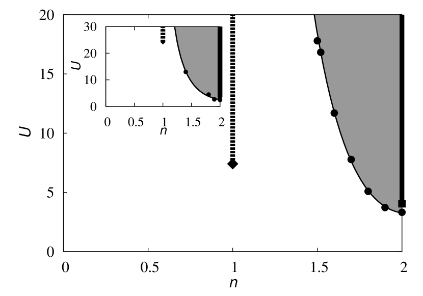
Figure 9: Phase diagram for the system with different bandwidths $R=0.5$ when $J/U=0.1$ (main) and $J/U=0.25$ (inset). The shaded region represents the OSM phase with one orbital localized and the other itinerant.

At half filling $(n=2)$, as introducing the Coulomb interaction, the Mott transition in the narrower band occurs to the OSM phase. Further increase of the interaction drives the system to the Mott insulating phase. If the total electron count is changed in the Mott insulating phase, holes are doped only in the wider band due to the strong correlations in the narrower band. Therefore, the OSM phase is stabilized even away from half filling. When the electron count approaches quarter filling, the holes are introduced in both bands, thus the system is driven to the metallic state. In contrast, the different type of the Mott insulating state appears beyond a certain critical point when the system is quarter-filled.

Up to now, we have restricted our discussion to the condition $J/U=0.1$ and $R=0.5$. If the Hund coupling is increased, orbital fluctuations are further suppressed. Therefore, it is expected that the OSM phase becomes more stable, while the Mott insulating phase at quarter filling becomes unstable. In fact, in comparison with the phase diagram for $J/U=0.1$ and $R=0.5$, the region of the OSM phase broadens and the critical point at quarter filling is increased, as shown in the inset of Fig. 9. The large difference of the bandwidths also suppresses orbital fluctuations, as discussed in the previous paper.[32] Therefore, the same phase diagram is expected to be obtained, where the wide OSM phase away from half filling is realized.

5 Summary

We have investigated the two-orbital Hubbard model with same and different bandwidths at zero temperature. By making use of the SFA, we have discussed the competition between the metallic and the insulating states in the system at arbitrary band fillings. We have found that the Mott transition occurs only at commensurate band fillings in the system with same bandwidths. On the other hand, in the system with different bandwidths, the OSM phase with one orbital localized and the other itinerant is stabilized in a certain parameter region. There are some open problems in the present study. One of the most important issues is magnetism of the system, which has not been treated here, since we have restricted our attention to the paramagnetic phase. This problem is under consideration.

Appendix A Formulation of the SFA

We briefly summarize the formulation of the SFA in order to discuss the Mott transition in the system without particle-hole symmetry. Here, by combining the numerical method with the analytic method, we describe the Mott insulating state in the framework of the SFA.

First, let us consider the free energy $F$ for the system as,

$$F/L=\Omega/L+\mu n,$$ (3)

where $L$ is the number of sites and $n$ is the electron count per site. The grand potential $\Omega$ is given as,

$$\Omega[{\bm{\Sigma}}] = \Gamma[{\bm{\Sigma}}]+{\rm Tr}\ln[-({\bf G}_{0}^{-1}-{\bm{\Sigma}})^{-1}],$$ (4)

where $\Gamma[{\bm{\Sigma}}]$ is the Legendre transformation of the Luttinger-Ward potential. [62] ${\bf G}_{0}$ and ${\bm{\Sigma}}$ are the bare Green function and the self-energy, respectively. The condition ${\partial\Omega[{\bm{\Sigma}}]}/{\partial{\bm{\Sigma}}}=0$ gives us the Dyson equation ${\bf G}^{-1}={\bf G}_{0}^{-1}-{\bm{\Sigma}}$, [62] where ${\bf G}$ is the full Green function. Note that the potential $\Gamma[{\bm{\Sigma}}]$ does not depend on the detail of the non-interacting Hamiltonian.[55] This enables us to introduce a reference system with the same interacting term. The Hamiltonian is explicitly given by ${\cal H}_{\rm ref}({\bf t}^{\prime})={\cal H}_{0}({\bf t}^{\prime})+{\cal H}^{\prime}$ with the parameter matrix ${\bf t}^{\prime}$. Then the grand potential is given as,

$$\Omega[{\bm{\Sigma}}({\bf t}^{\prime})] = \Omega({\bf t^{\prime}})$$ (5)

$$+ {\rm Tr}\ln\left[-(\omega+\mu-{\bf t}-{\bm{\Sigma}}({\bf t^{\prime}}))^{-1}\right]$$

$$- {\rm Tr}\ln\left[-(\omega+\mu-{\bf t}^{\prime}-{\bm{\Sigma}}({\bf t^{\prime}}))^{-1}\right],$$

where $\Omega({\bf t}^{\prime})$ and ${\bm{\Sigma}}({\bf t}^{\prime})$ are the grand potential and the self-energy for the reference system. The condition $\partial\Omega[{\bm{\Sigma}({\bf t}^{\prime})}]/\partial{\bf t}^{\prime}=0$ gives us an appropriate reference system in the framework of the SFA, which approximately describes the original correlated system.

Here, we introduce a two-site Anderson impurity model as the reference system, which has successfully described strongly correlated electron systems in the infinite dimensions. [55, 56, 63, 64, 54, 30] The Hamiltonian of the reference system is explicitly given as

$${\cal H}_{\rm ref} = \sum_{i}{\cal H}_{\rm ref}^{(i)},$$ (6)

$${\cal H}_{\rm ref}^{(i)} = \sum_{\alpha\sigma}\varepsilon^{c}_{\alpha}c^{\dagger}_{i\alpha\sigma}c_{i\alpha\sigma}+\sum_{\alpha\sigma}\varepsilon^{a}_{\alpha}a^{{\dagger}}_{i\alpha\sigma}a_{i\alpha\sigma}$$ (7)

$$+ \sum_{\alpha\sigma}V_{\alpha}(c^{\dagger}_{i\alpha\sigma}a_{i\alpha\sigma}+H.c.)+{\cal H}_{i}^{\prime},$$

where $a^{{\dagger}}_{i\alpha\sigma}(a_{i\alpha\sigma})$ creates (annihilates) an electron with spin $\sigma$ and orbital $\alpha$, which is connected to the $i$th site in the original lattice. The grand potential per site is rewritten as,

$$\Omega/L = \Omega_{\rm imp}-2\sum_{\alpha}\sum_{m}g(\omega^{\prime}_{\alpha m})-2\sum_{\alpha}g(\varepsilon^{a}_{\alpha}-\mu)$$ (8)

$$+ 2\sum_{\alpha}\sum_{m}\int^{-\infty}_{\infty}dz\rho_{\alpha}(z)g[\omega_{\alpha m}(z)],$$

$$g(x) = -T\ln[1+\exp(-x/T)]$$ (9)

where $\Omega_{\rm imp}$ is the grand potential for the reference system and $\omega_{\alpha m}(z)$ $[\omega^{\prime}_{\alpha m}]$ are the poles of Green function $G$ $(G^{\prime})$ for the original (reference) system. The Green function of the reference system is given as,

$$G^{\prime}_{\alpha}(\omega) = [\omega+\mu-\varepsilon^{c}_{\alpha}-\frac{V_{\alpha}^{2}}{\omega+\mu-\varepsilon^{a}_{\alpha}}-\Sigma_{\alpha}(\omega)]^{-1},$$ (10)

where $\Sigma_{\alpha}(\omega)$ is the self-energy for the $\alpha$th orbital. On the other hand, the full Green function for the original system is given as,

$$G_{\alpha}(\omega) = \int dz\rho_{\alpha}(z)G_{\alpha}(\omega;z),$$ (11)

$$G_{\alpha}(\omega;z) = [\omega+\mu-z-\Sigma_{\alpha}(\omega)]^{-1},$$ (12)

where $\rho_{\alpha}(x)$ is the density of states for the bare $\alpha$th orbital. Note that the following differential equation is efficient to deduce the poles $\omega_{\alpha m}(z)$ of the Green function for the original system,

$$\frac{d\omega_{\alpha m}(z)}{dz}=\left(1-\frac{\partial\Sigma_{\alpha}(\omega)}{\partial\omega}\right)^{-1}_{\omega=\omega_{\alpha m}(z)}.$$ (13)

By solving these differential equations, we estimate the free energy [Eq. (3)] numerically. The variational parameters ${\bm{\lambda}}=(\mu,V_{\alpha},\epsilon^{c}_{\alpha},\epsilon^{a}_{\alpha}$) are determined by the condition $\partial F/\partial{\bm{\lambda}}=0$, which corresponds to the stationary point in the parameter space.

In the framework of SFA, the variational parameters for the metallic and the OSM states can be determined numerically. In contrast, it may be difficult to determine unique variational parameters for the Mott insulating state, as discussed above. To overcome this, we make use of the analytical and the numerical methods.

For simplicity, we consider the two-orbital model with $J/U=0$ at quarter filling. Recall that the Mott insulating phase is simply represented in the atomic limit, by taking into account local electron correlations. Since the four one-electron states $c^{\dagger}_{\alpha\sigma}|0\rangle$ are degenerate $(\varepsilon^{c}_{1}=\varepsilon^{c}_{2})$, the ground state $|\Phi_{G}\rangle$ in the reference system [eq. (7)] should be given as

$$|\Phi_{G}\rangle=\sum_{\alpha\sigma}\sqrt{n_{\alpha}}c^{\dagger}_{\alpha\sigma}|0\rangle,$$ (14)

where $n_{\alpha}$ is the expectation value of band fillings for the $\alpha$th orbital, which satisfies the constraint $\sum_{\alpha\sigma}n_{\alpha}=1$.

The Green function and the self-energy for the reference system [eq. (7)] are given as

$$G^{\prime}_{\alpha}(\omega) = \frac{n_{\alpha}}{\omega+\mu+\varepsilon^{c}_{\alpha}}+\frac{1-n_{\alpha}}{\omega+\mu+\varepsilon^{c}_{\alpha}-U},$$ (15)

$$\Sigma_{\alpha}(\omega) = \omega+\mu+\varepsilon^{c}_{\alpha}-1/G^{\prime}_{\alpha}(\omega).$$ (16)

The Green function for the original system is then written as $G_{\alpha}(\omega)=\int dz\rho_{\alpha}(z)G_{\alpha}(\omega;z)$ with

$$G_{\alpha}(\omega;z) = \frac{1}{\omega+\mu-z-\Sigma_{\alpha}(\omega)}$$ (17)

$$= \sum_{l=\pm}\frac{R^{\alpha}_{l}(z)}{\omega-\xi_{l}^{\alpha}(z)},$$

where

$$\xi_{\pm}^{\alpha}(z) = \frac{1}{2}\bigg{(}U+z-\varepsilon^{c}_{\alpha}\pm\eta(z)\bigg{)}-\mu,$$

$$R_{\pm}^{\alpha}(z) = \frac{1}{2}\bigg{(}1\pm\frac{z+\varepsilon^{c}_{\alpha}+U(1-2n_{\alpha})}{\eta(z)}\bigg{)},$$

$$\eta(z) = \sqrt{U^{2}+2(1-2n_{\alpha})(z+\varepsilon^{c}_{\alpha})U+(z+\varepsilon^{c}_{\alpha})^{2}}.$$

This formula is equivalent to the Hubbard-I type approximation. Finally, we obtain the free energy per site for the system as

$$F/L=\sum_{\alpha}(\mu+\varepsilon^{c}_{\alpha})(1-n_{\alpha})+\mu\sum_{\alpha}n_{\alpha}$$

$$+\sum_{\alpha}\sum_{l=\pm}\int dz\rho_{\alpha}(z)\xi_{l}^{\alpha}(z)\theta[-\xi^{\alpha}_{l}(z)].$$ (18)

At the stationary point in the free energy, three conditions are obtained as,

$$1 = \sum_{l=\pm}\int dz\rho_{\alpha}(z)\theta[-\xi^{\alpha}_{l}(z)],$$ (19)

$$n_{\alpha} = \sum_{l=\pm}\int dz\rho_{\alpha}(z)R_{l}^{\alpha}(z)\theta[-\xi^{\alpha}_{l}(z)],$$ (20)

We wish to note that the right hand side of eq. (20) is equivalent to $\int^{i\infty}_{-i\infty}G_{\alpha}(\omega)d\omega/2\pi i$ for each orbital. This implies that $n_{\alpha}$ is identical to the electron count for the lattice system.

As described above, the chemical potential is difficult to be determined uniquely in the insulating phase. In fact, the condition $\partial F/\partial\mu=0$ is satisfied in the case $W_{\alpha}/2\lesssim\mu\lesssim U-W_{\alpha}/2\;(U>>W_{\alpha})$, which originates from the presence of the Hubbard gap. Here, we set the chemical potential as $\mu=U/2$. Then the condition eq. (19) is always satisfied, and eq. (20) is rewritten as

$$n_{\alpha}=\int dz\rho_{\alpha}(z)R_{-}^{\alpha}(z).$$ (21)

By solving the self-consistent equations eq. (21), $\sum_{\alpha\sigma}n_{\alpha}=1$, and $\varepsilon^{c}_{1}=\varepsilon^{c}_{2}$, we can describe the Mott insulating phase in the framework of the SFA.

References

- [1] M. Imada, A. Fujimori and Y. Tokura: Rev. Mod. Phys. 70 (1998) 1039.
- [2] S. Kondo, D. C. Johnston, C. A. Swenson, F. Borsa, A. V. Mahajan, L. L. Miller, T. Gu, A. I. Goldman, M. B. Maple, D. A. Gajewski, E. J. Freeman, N. R. Dilley, R. P. Dickey, J. Merrin, K. Kojima, G. M. Luke, Y. J. Uemura, O. Chmaissem and J. D. Jorgensen: Phys. Rev. Lett. 78 (1997) 3729.
- [3] H. Kaps, N. Büttgen, W. Trinkl, A. Loidl, M. Klemm and S. Horn: J. Phys.: Condens. Matter 13 (2001) 8497.
- [4] M. Isoda and S. Mori: J. Phys. Soc. Jpn. 69 (2000) 1509.
- [5] S. Fujimoto: Phys. Rev. B 64 (2001) 085102.
- [6] H. Tsunetsugu: J. Phys. Soc. Jpn. 71 (2002) 1844.
- [7] Y. Yamashita and K. Ueda: Phys. Rev. B 67 (2003) 195107.
- [8] S. Nakatsuji et al.: Phys. Rev. Lett. 90 (2003) 137202; S. Nakatsuji and Y. Maeno: Phys. Rev. Lett. 84 (2000) 2666.
- [9] Y. Kobayashi, S. Taniguchi, M. Kasai, M. Sato, T. Nishioka and M. Kontani: J. Phys. Soc. Jpn 65 (1996) 3978.
- [10] K. Sreedhar: et al., J. Solid State Comm. 110 (1994) 208; Z. Zhang, et al.: J. Solid State Comm. 108 (1994) 402; 117 (1995) 236.
- [11] V. I. Anisimov, I. A. Nekrasov, D. E. Kondakov, T. M. Rice and M. Sigrist: Eur. Phys. J. B 25 (2002) 191.
- [12] M. S. Laad, L. Craco and E. Müller-Hartmann: Phys. Rev. B 73 (2006) 045109.
- [13] A. Liebsch: Europhys. Lett. 63 (2003) 97.
- [14] A. Liebsch: Phys. Rev. Lett. 91 (2003) 226401.
- [15] A. Liebsch: Phys. Rev. B 70 (2004) 165103.
- [16] M. Sigrist and M. Troyer: Eur. Phys. J. B 39 (2004) 207.
- [17] S. Okamoto and A. J. Millis: Phys. Rev. B 70 (2004) 195120.
- [18] Z. Fang, N. Nagaosa and K. Terakura: Phys. Rev. B 69 (2004) 45116.
- [19] A. Koga, N. Kawakami, T. M. Rice and M. Sigrist: Phys. Rev. Lett. 92 (2004) 216402.
- [20] A. Koga, N. Kawakami, T. M. Rice and M. Sigrist: Phys. Rev. B 72 (2005) 045128.
- [21] A. Koga, N. Kawakami, T. M. Rice and M. Sigrist: Phyisica B 359-361 (2005) 738.
- [22] A. Koga, K. Inaba and N. Kawakami: Prog. Theor. Phys. Suppl. 160 (2005) 253.
- [23] M. Ferrero, F. Becca, M. Fabrizio and M. Capone: Phys. Rev. B 72 (2005) 205126.
- [24] L. de’ Medici, A. Georges and S. Biermann: Phys. Rev. B 72 (2005) 205124.
- [25] R. Arita and K. Held: Phys. Rev. B 72 (2005) 201102(R).
- [26] C. Knecht, N. Blümer and P. G. J. van Dongen: Phys. Rev. B 72 (2005) 081103(R).
- [27] A. Liebsch: Phys. Rev. Lett. 95 (2005) 116402.
- [28] S. Biermann, L. de’ Medici and A. Georges: Phys. Rev. Lett. 95 (2005) 206401.
- [29] Y. Tomio and T. Ogawa: J. Lumin. 112 (2005) 220.
- [30] K. Inaba, A. Koga, S. Suga and N. Kawakami: J. Phys. Soc. Jpn. 74 (2005) 2393.
- [31] A. Ruëgg, M. Indergand, S. Pilgram and M. Sigrist: Eur. Phys. J. B 48 (2005) 55.
- [32] K. Inaba and A. Koga: Phys. Rev. B 73 (2006) 155106.
- [33] P. G. J. van Dongen, C. Knecht and N. Blümer: phys. stat. sol. 243 (2006) 116.
- [34] P. Werner and A. J. Millis: Phys. Rev. B 74 (2006) 155107.
- [35] L. Balicas, S. Nakatsuji, D. Hall, Z. Fisk, Y. Maeno and D. J. Singh: Phys. Rev. Lett. 95 (2005) 196407.
- [36] J. S. Lee, S. J. Moon, T. W. Noh, S. Nakatsuji and Y. Maeno: Phys. Rev. Lett. 96 (2006) 057401.
- [37] J. Bünemann and W. Weber, Phys. Rev. B 55, 4011 (1997); J. Bünemann and W. Weber and F. Gebhard, ibid 57, 6896 (1998).
- [38] O. Gunnarsson, E. Koch and R. M. Martin: Phys. Rev. B 54 (1996) 11026.
- [39] G. Kotliar and H. Kajueter: Phys. Rev. B 54 (1996) R14221.
- [40] M. J. Rozenberg: Phys. Rev. B 55 (1997) R4855.
- [41] H. Hasegawa: J. Phys. Soc. Jpn. 66 (1997) 3522.
- [42] A. Klejnberg and J. Spalek: Phys. Rev. B 57 (1998) 12041.
- [43] J. E. Han, M. Jarrel and D. L. Cox: Phys. Rev. B 58 (1998) R4199.
- [44] Y. Imai and N. Kawakami: J. Phys. Soc. Jpn 70 (2001) 2365.
- [45] A. Koga and Y. Imai and N. Kawakami: Phys. Rev. B 66 (2002) 165107; J. Phys. Soc. Jpn. 72 (2003) 1306.
- [46] S. Florens, A. Georges, G. Kotliar and O. Parcollet: Phys. Rev. B 66 (2002) 205102.
- [47] S. Florens and A. Georges: Phys. Rev. B 66 (2002) 165111.
- [48] Y. Ono, M. Potthoff and R. Bulla: Phys. Rev. B 67 (2003) 035119.
- [49] T. Pruschke and R. Bulla: Eur. Phys. J. B 44 (2005) 217.
- [50] T. Momoi and K. Kubo: Phys. Rev. B 58 (1998) R567.
- [51] K. Held and D. Vollhardt: Eur. Phys. J. B 5 (1998) 473.
- [52] S. Sakai, R. Arita, K. Held and H. Aoki: Phys. Rev. B 74 (2006) 155102.
- [53] V. S. Oudovenko and G. Kotliar: Phys. Rev. B 65 (2002) 075102.
- [54] K. Inaba, A. Koga, S.-I. Suga and N. Kawakami: Phys. Rev. B 72 (2005) 085112.
- [55] M. Potthoff: Eur. Phys. J. B 32 (2003) 429.
- [56] M. Potthoff: Eur. Phys. J. B 36 (2003) 335.
- [57] K. Pozgǎjčić: cond-mat/0407172.
- [58] M. Aichhorn, H. G. Evertz, W. von der Linden and M. Potthoff: Phys. Rev. B 70 (2004) 235107.
- [59] D. Senechal, P.-L. Lavertu, M.-A. Marois and A.-M. S. Tremblay: Phys. Rev. Lett. 94 (2005) 156404.
- [60] M. Aichhorn, E. Y. Sherman and H. G. Evertz: Phys. Rev. B 72 (2005) 155110.
- [61] M. Aichhorn and E. Arrigoni: Europhys. Lett. 72 (2005) 117.
- [62] J. M. Luttinger: Phys. Rev. 118 (1960) 1417.
- [63] M. Balzer and M. Potthoff: Phyisica B 359-361 (2005) 768.
- [64] W. Koller, D. Meyer, A. C. Hewson and Y. Ono: Phyisica B 359-361 (2005) 795.