Multipole expansion of the electrostatic interaction between charged colloids at interfaces

Abstract

The general form of the electrostatic potential around an arbitrarily charged colloid at a flat interface between a dielectric and a screening phase (such as air and water, respectively) is analyzed in terms of a multipole expansion. The leading term is isotropic in the interfacial plane and varies with $d^{-3}$ where $d$ is the in–plane distance from the colloid. The effective interaction potential between two arbitrarily charged colloids is likewise isotropic and $\propto d^{-3}$, thus generalizing the dipole–dipole repulsion first found for point charges at water interfaces. Anisotropic, attractive interaction terms can arise only for higher powers $d^{-n}$ with $n\geq 4$. The relevance of these findings for recent experiments is discussed.

I Introduction

The self–assembly of stably trapped, sub-$\mu$m colloidal particles at water–air or water–oil interfaces has gained much interest in recent years. For the specific case of charge–stabilized colloids at interfaces, the repulsive part of their mutual interaction resembles a dipole–dipole interaction at large separations. This may be understood theoretically by approximating the colloid as a point charge located either right at the interface Stil61 ; Hur85 (i.e. assuming charges on the colloid–water interface) and/or above the interface Ave00a (i.e. assuming charges on the colloid–air/oil interface). Additionally, the formation of metastable mesostructures with such colloids point to the possible existence of intercolloidal attractions far beyond the range of van–der–Waals forces Gom05 ; Che05 ; Che06 , however, care must be taken to avoid contaminations of the interface which lead to colloid mesostructures with similar appearance Fer04 . Previous work For04 ; Oet05 ; Oet05a ; Wue05 ; Dom07 aimed at relating this attractive minimum to capillary interactions due to interfacial deformations caused by a homogeneous surface charge on the colloids but with no conclusive answer. In recent work Che05 ; Che06 , it was experimentally shown that the charge–carrying surface groups used for charge–stabilizing polystyrene colloids are actually distributed quite inhomogeneously and patchily over the colloid surface. Thus it was speculated in Refs. Che05 ; Che06 that through this inhomogeneous charge distribution like–charged colloids could acquire effective dipole moments in the interface plane and attractive electrostatic interactions of dipole–dipole type could arise which might overcome the repulsion at shorter distances.

Motivated by the finding of inhomogeneous surface charge on colloids, we extend the asymptotic results for the electrostatic potential and interaction of point charges at water interfaces Hur85 to the general case of an arbitrary, localized colloidal charge distribution using a multipole expansion. The presence of the interface leads to restrictions in the multipole coefficients of the potential around a single colloid and of the interaction energy between two colloids. In particular, we find that the leading term in the effective interaction energy between two colloids at lateral distance $d$ is isotropic in the interfacial plane, repulsive and $\propto d^{-3}$ regardless of the inhomogeneities of the charge distribution in the colloids. Angular dependencies enter the effective interaction potential only in higher orders.

II Electrostatics at water interfaces

II.1 A toy model: water as a perfect conductor

For a quick insight on the effect of an interface on the multipole expansion of the electrostatic potential, we consider the water phase being a perfect conductor. The flat interface is located at $z=0$ and the colloid is modelled by a fixed charge distribution $\rho_{\rm C}(\mathbf{r})$ above the water phase. The boundary condition at $z=0$ simply implies that there is no tangential (or in–plane) electric field and the potential for $z>0$ can be obtained with the method of image charges. Therefore, the effective (real + image) charge distribution is spatially localized and can be enclosed in a ball of finite radius $R$ (see Fig. 1 with $\kappa^{-1}\to 0$). In standard spherical coordinates $(s,\theta,\varphi)$ measured from the center of this ball, the potential in the upper phase for $s>R$ can be written as a multipole expansion (in the remainder of the paper, the $+$($-$) index will refer to evaluation in the upper(lower) phase):

$$\Phi_{+}(s,\theta,\varphi)=\sum_{\ell m}a_{\ell m}s^{-\ell-1}Y_{\ell m}(\theta,\varphi)\;,$$ (1)

in terms of normalized spherical harmonics $Y_{\ell m}$. The boundary condition of vanishing in–plane electric field at the interface ($\theta=\pi/2$) implies $a_{\ell m}=0$ for $\ell+m$ even. Thus, the monopole vanishes ($a_{00}=0$) as well as the in–plane dipole ($a_{1\,\pm 1}=0$), and the leading decay is described generically by a dipole perpendicular to the interface ($a_{10}\neq 0$). Consider a second, identical colloid located at an in–plane position $\mathbf{d}=(d_{x},d_{y})$. The total potential $\Phi_{+}$ is now the linear superposition of the single–particle potentials $\Phi_{+}^{0}$ by each colloid, and the electrostatic energy of the two–particle configuration is

$$U=U^{0}+\int d^{3}r\,\rho_{\rm C}(\mathbf{r})\,\Phi_{+}^{0}({\mathbf{r}}+{\mathbf{d}})\;,$$ (2)

where $U^{0}$ is the energy in the limit $d\to\infty$. Taylor expanding $\Phi_{+}^{0}$ about ${\mathbf{r}}={\mathbf{0}}$ one obtains to leading order in $1/d$

$$U-U^{0}\sim\frac{p_{z}^{2}}{2d^{3}}\qquad(d\to\infty),$$ (3)

where $p_{z}=2\int d^{3}r\,z\,\rho_{\rm C}(\mathbf{r})=a_{10}\sqrt{3/(4\pi)}$ is the dipolar moment of $\rho_{\rm C}$ and its image charge in the direction normal to the interface. This dipole–dipole interaction energy differs by a factor of one-half from the textbook result because

Figure 1: Geometrical configuration of the electrostatic problem: the potential is calculated in the domain outside the sphere of radius $R$, which encloses the colloidal particle. The flat interface at $z=0$ separates an upper dielectric phase (dielectric constant $\epsilon_{+}$) from a lower electrolytic phase (dielectric constant $\epsilon_{-}$, Debye screening length $\kappa^{-1}$).

II.2 Water as a conductor with linear screening

The image charge construction in the case of perfectly conducting water provides an intuitive explanation of the origin of the normal dipole and the absence of an in–plane dipole. In the following we demonstrate that this finding still holds in the more realistic case of water being an electrolyte and the colloidal particle having an arbitrary shape, possibly protruding into the region $z<0$, with given charge distribution and dielectric properties. Assuming linear screening, the electrostatic potential satisfies $(\Delta-\kappa_{\pm}^{2})\Phi_{\pm}(\mathbf{r})=0$ with $\kappa_{+}=0$ and $\kappa_{-}=\kappa$ being the inverse screening length in water. Using standard cylindrical coordinates $(r,z,\varphi)$, we search for a solution outside a ball of radius $R$ whose center is the coordinate origin and which encloses the colloid (see Fig. 1) with the boundary conditions that the potential (i) vanishes at infinity, (ii) reduces to a given potential $\Phi_{R}(\theta,\varphi)$ at the surface of the ball $s=R$, (iii) is continuous at the interface $z=0$, and (iv) that the associated electric displacement perpendicular to the interface is continuous, i.e.,

$$\epsilon_{+}\left.\frac{\partial\Phi_{+}}{\partial z}\right|_{z=0} = \epsilon_{-}\left.\frac{\partial\Phi_{-}}{\partial z}\right|_{z=0}\qquad(r>R).$$ (4)

The function $\Phi_{R}(\theta,\varphi)$ is determined by the solution of the electrostatic problem inside the ball and contains the relevant information on the precise geometrical and electric properties of the particle. By decomposing the problem in the full domain into the solution of problems in simpler domains (the exterior of the sphere $s=R$ and each of the halfspaces defined by $z=0$ (details can be found in App. A), one can finally write the solution as the superposition $\Phi_{\pm}(\mathbf{r})=\Phi^{\rm cyl}_{\pm}(r,z,\varphi)+\Phi^{\rm sph}_{\pm}(s,\theta,\varphi)$, where the contribution $\Phi^{\rm cyl}_{\pm}(r,z,\varphi)$ (using cylindrical coordinates) is given by

$$\Phi^{\rm cyl}_{\pm}(r,z,\varphi) = \sum_{m=-\infty}^{+\infty}e^{im\varphi}\int_{0}^{\infty}\!\!\!dq\,A_{m}(q)J_{|m|}(qr)\,{\rm e}^{-K_{\pm}z}$$

with $K_{\pm}=\pm\sqrt{q^{2}+\kappa_{\pm}^{2}}$, and the contribution $\Phi^{\rm sph}_{\pm}$ (using spherical coordinates) reads

$$\Phi^{\rm sph}_{\pm}(s,\theta,\varphi) = \sum_{\ell=0}^{\infty}\sum_{m=-\ell}^{+\ell}C_{\ell m}^{\pm}{\cal R}_{\ell}^{\pm}(s)Y_{\ell m}(\theta,\varphi)$$ (6)

$$\left({\cal R}_{\ell}^{\pm}(s)=s^{\ell}\frac{d^{\ell}}{(s\,ds)^{\ell}}\left[\frac{{\rm e}^{-\kappa_{\pm}s}}{s}\right]\right).$$

The coefficients $C_{\ell m}^{\pm}$ are given by

$$C_{\ell m}^{\pm} = [1-(-1)^{\ell-m}]\int_{0}^{2\pi}d\varphi\int_{0}^{\pm 1}d(\cos\theta)\,Y_{\ell m}^{*}(\theta,\varphi)\times\mbox{}$$ (7)

$$\mbox{}\left[\Phi_{R}(\theta,\varphi)-\Phi_{\pm}^{\rm cyl}(r=R\sin\theta,z=R\cos\theta,\varphi)\right],\qquad$$

such that $\Phi^{\rm sph}_{\pm}=0$ at $z=0$, $\Phi_{\pm}(s=R)=\Phi_{R}(\theta,\varphi)$, and the boundary conditions (i)–(iii) are satisfied automatically. The coefficients $A_{m}(q)$ in the expression for $\Phi_{\pm}^{\rm cyl}$ (Eq. (II.2)) must be chosen to enforce the boundary condition (4). This condition can be extended to the region $0<r<R$ by continuing the fields $\Phi_{\pm}(\mathbf{r})$ with any virtual solution into the interior of the ball, $s<R$. The precise form of the continuation is irrelevant, since the solution outside the ball depends only on the potential at the surface of the ball, $\Phi_{R}(\theta,\varphi)$ (Faraday’s cage effect). Thus, by using orthonormality and closure of the set of Bessel functions $\{J_{|m|}(qr)\}_{q\in[0,\infty)}$ in the domain $0<r<\infty$, Eq. (4) can be solved for the coefficients $A_{m}(q)$:

$$A_{m}(q) = \frac{q\,\sum_{\ell=0}^{\infty}\left[\epsilon_{+}\hat{C}^{+}_{\ell m}\gamma^{+}_{\ell m}(q)-\epsilon_{-}\hat{C}^{-}_{\ell m}\gamma^{-}_{\ell m}(q)\right]}{\epsilon_{+}q+\epsilon_{-}\sqrt{q^{2}+\kappa^{2}}},\qquad$$ (8)

with $\hat{C}^{\pm}_{\ell m}:=-{\rm e}^{-im\varphi}\partial_{\theta}Y_{\ell m}(\theta=\pi/2,\varphi)\,C^{\pm}_{\ell m}$ and $\gamma^{\pm}_{\ell m}(q):=\int_{R}^{+\infty}dr\;{\cal R}^{\pm}_{\ell}(r)\,J_{|m|}(qr)$, which are the Hankel transforms of the radial dependence of the spherical part $\Phi_{\pm}^{\rm sph}$ (see Eq. (6)) continued into the region $s<R$ by zero. Eq. (8) is not the explicit expression for the coefficients $A_{m}(q)$ because they appear implicitly also in the coefficients $C^{\pm}_{\ell m}$, see Eq. (7), but it does provide their dependence on $q$. In particular, for $\ell-m$ odd (i.e., when $C^{\pm}_{\ell m}\neq 0$), the functions $\gamma^{\pm}_{\ell m}(q)$ possess a Taylor expansion around $q=0$ with the lowest term being of order $q^{|m|}$, so that

$$A_{m}(q)=\sum_{j=0}^{\infty}a_{jm}q^{j},\qquad\textrm{with $a_{jm}=0$ if }j\leq|m|.$$ (9)

The existence of a Taylor expansion in $q$ of the coefficients $A_{m}(q)$ allows to extract the large–$r$ behavior of the potential and the $z$–component of the electric field at the interface. Introducing the factors

$${\cal J}_{jm} := \lim_{z\to 0}\int_{0}^{\infty}dp\,p^{j}J_{|m|}(p){\rm e}^{-zp}=\frac{2^{j}\,\Gamma\left(\frac{|m|+j+1}{2}\right)}{\Gamma\left(\frac{|m|-j+1}{2}\right)}$$

and inserting the expansion (9) into the corresponding definitions of the fields, one obtains

$$\Phi_{\pm}(r,\varphi,z=0) \sim \sum_{j=0}^{\infty}\;\sum_{m=-j+1}^{j-1}\frac{{\rm e}^{im\varphi}}{r^{j+1}}\,a_{jm}{\cal J}_{jm},$$

$$\sim \mbox{}-\frac{a_{20}}{r^{3}}-\frac{3}{r^{4}}\sum_{\pm}a_{3\pm 1}{\rm e}^{\pm i\varphi}\cdots,$$

$$\left.\frac{\partial\Phi_{+}}{\partial z}\right|_{z=0} \sim \sum_{j,m}\frac{{\rm e}^{im\varphi}}{r^{j+2}}\,\left[r^{j+1}{\cal R}^{+}_{j}(r)\hat{C}^{+}_{jm}-a_{jm}{\cal J}_{j+1,m}\right],$$

$$\sim \frac{a_{10}+\hat{C}^{+}_{10}}{r^{3}}+\frac{3}{r^{4}}\sum_{\pm}(a_{2\pm 1}+\hat{C}^{+}_{2\pm 1}){\rm e}^{\pm i\varphi}\cdots,$$

where we have used that $C^{+}_{jm}=0$ if $|m|=j$ and $\hat{C}^{+}_{jm}=0$ whenever ${\cal J}_{j+1,m}=0$. Therefore, both the potential and the normal component of the electric field at the interface are asymptotically dominated by an angular–independent decay $\propto 1/r^{3}$; anisotropic behavior arises only in subleading terms. By continuity, this conclusion also holds asymptotically for the fields at a fixed height $h$ above or below the interface ($r\gg|h|$).

This result is not exclusive of the single–particle configuration: if there are several particles at the interface, one can surround each of them by a ball of radius $R$ and the solution $\Phi(\mathbf{r})$ of the electrostatic problem will be written as a superposition of single–particle potentials determined by the total potential at the surface of each ball (in general different from the potential $\Phi_{R}(\theta,\varphi)$ in the single–particle configuration). For each of these single–particle potentials the expansion (9) still holds, since it does not depend on the precise value of the potential at the balls.

II.3 An illustrative 2d example

We calculated the electrostatic potential for an inhomogeneously charged cylinder at an air–water interface (see the inset of Fig. 2 for some definitions). Because of its two–dimensional nature, this problem is amenable to a numerical treatment. Here, the multipole expansion at the interface gives $\Phi_{\pm}(z=0)\sim a_{0}\ln|x|+p_{x}/x+q_{xx}/x^{2}+\dots$ and $\left.\partial\Phi_{+}/\partial z\right|_{z=0}\sim p_{z}/x^{2}+\dots$. The numerical solution for $\Phi_{\pm}$ shows that the in–plane dipole term $\propto x^{-1}$ is absent and the asymptotic expansion starts with the quadrupolar term (see Fig. 2). The asymptotics for $\left.\partial\Phi_{+}/\partial z\right|_{z=0}$ (not shown) also contains the term $\propto x^{-2}$, which is interpreted as the effect of a counter–ion generated dipole component $p_{z}$ perpendicular to the interface. These findings, most notably the absence of $p_{x}$, match the previous ones in three dimensions.

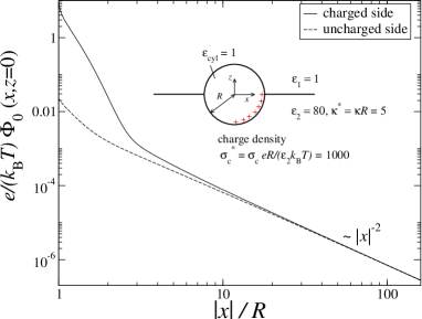
Figure 2: Potential along the interface for an inhomogeneously charged cylinder half–immersed in water. Maxwell’s equations hold in the upper phase and the cylinder, the Poisson–Boltzmann equation holds in the lower phase. The parameters are given in the inset, the numerical calculations have been done using FEMLAB.

II.4 The effective interaction energy

The free energy functional of a multiparticle configuration in the linear screening approximation reads ShHo90

$$F[\Phi]=\int d^{3}r\,\left[\rho_{\rm C}({\mathbf{r}})\Phi-\frac{\epsilon({\mathbf{r}})}{8\pi}\left[\kappa^{2}({\mathbf{r}})\Phi^{2}+|\nabla\Phi|^{2}\right]\right],$$ (11)

where the charge density $\rho_{\rm C}({\mathbf{r}})$ is localized on the colloidal particles. This includes the electrostatic energy as well as the entropy associated to the ion distribution. The extremum of $F[\Phi]$ provides the field equation in thermal equilibrium, $\nabla\cdot[\epsilon\nabla\Phi]=\epsilon\kappa^{2}\Phi-4\pi\rho_{C}$. With the help of this equation, the free energy in equilibrium simplifies to

$$F_{\rm eq}(\{{\mathbf{x}}_{\alpha}\})=\frac{1}{2}\int d^{3}r\,\rho_{\rm C}({\mathbf{r}})\Phi({\mathbf{r}}),$$ (12)

which is known as the ”potential of mean force” for the degrees of freedom ${\mathbf{x}}_{\alpha}$ (position of the center of a ball of radius $R$ enclosing the $\alpha$-th particle). One may decompose $F_{\rm eq}=F^{0}+\delta F$, where $F^{0}$ is the equilibrium free energy in the limit $|{\mathbf{x}}_{\alpha}-{\mathbf{x}}_{\beta}|\to\infty$ (isolated particles). The total potential can be similarly written as $\Phi=\sum_{\alpha}\Phi^{0}_{\alpha}+\delta\Phi$, where $\Phi^{0}_{\alpha}({\mathbf{r}})$ denotes the potential field generated by the $\alpha$-th particle in isolation and $\delta\Phi({\mathbf{r}};\{{\mathbf{x}}_{\alpha}\})$ is the total perturbation induced by the presence of other particles. Due to the linear nature of the problem, the perturbation $\delta\Phi$,

$$\delta\Phi({\mathbf{r}})=\sum_{\alpha\neq\beta}\int_{|{\mathbf{r}}^{\prime}-{\mathbf{x}}_{\alpha}|<R}d^{3}r^{\prime}\,G_{\alpha\beta}({\mathbf{r}},{\mathbf{r}^{\prime}})\Phi^{0}_{\beta}({\mathbf{r}}^{\prime}),$$ (13)

can be written in terms of a generalized susceptibility $G_{\alpha\beta}({\mathbf{r}},{\mathbf{r}}^{\prime})$ depending on the precise shape and charge distribution of the particles.

Since $\Phi^{0}({\mathbf{r}})$ near the interface exhibits asymptotically an isotropic decay $\propto 1/r^{3}$, $\delta\Phi({\mathbf{r}};\{{\mathbf{x}}_{\alpha}\})$ depends only on $d_{\alpha\beta}=|{\mathbf{x}}_{\alpha}-{\mathbf{x}}_{\beta}|$ (and not on the orientation of ${\mathbf{x}}_{\alpha}-{\mathbf{x}}_{\beta}$) in the asymptotic limit $d_{\alpha\beta}\to\infty$. Furthermore, $\delta\Phi$ is rescaled by a factor $\lambda^{-3}$ if all distances $d_{\alpha\beta}$ are rescaled simultaneously by a factor $\lambda$. From Eq. (12) the same property holds for $\delta F(\{{\mathbf{x}}_{\alpha}\})$. In particular, for a two–particle configuration this yields an asymptotic potential of mean force of the form

$$F_{\rm eq}(d)-F^{0}\sim\frac{B}{d^{3}}\qquad(d\to\infty),$$ (14)

and the constant $B$ is positive for like particles. In analogy with Eq. (3), it is natural to interpret this expression as the interaction energy between two effective dipoles perpendicular to the interface.

III Discussion and Conclusion

We have shown that the form of the multipole expansion of the potential around a charged colloid and of the effective interaction energy between two colloids trapped at a water interface is qualitatively different from the situation in bulk. The dominating interaction terms can be qualitatively understood by assuming water to be a perfect conductor. The leading interaction term between the colloids a distance $d$ apart is of dipole–dipole type ($\propto d^{-3}$) and isotropic in the interfacial plane. In other words, even if the charges on the colloid surface are distributed arbitrarily the counterions arrange themselves such that asymptotically the configuration corresponds to an effective dipole perpendicular to the interface. Orientation–dependent interactions and thus possible attractions for like–charged colloids only arise in subleading order.

This is in marked contrast to the analysis of the experiment reported in Refs. Che05 ; Che06 . Motivated by the experimentally found inhomogenous surface charge, it was pictorially suggested (see Fig. 1 in Ref. Che05 ) that spontaneous fluctuations in the colloid’s orientation would generate (via an instantaneously equilibrating counterion cloud) effective in–plane dipoles $\mathbf{p}_{i}$ with corresponding interactions $\propto[d^{2}({\mathbf{p}}_{1}\cdot{\mathbf{p}}_{2})-3({\mathbf{d}}\cdot{\mathbf{p}}_{1})({\mathbf{d}}\cdot{\mathbf{p}}_{2})]/d^{5}$. After averaging over the orientation fluctuations, such an interaction would lead to an effective, isotropic attraction competing with the isotropic dipole–dipole repulsion. According to the model worked out by the authors, the total interaction potential would exhibit an attractive minimum due to the effect of the fluctuating in–plane dipoles at rather small distances ($d\simeq 2.2$ colloid radii $R_{\rm C}$, so small that already the use of a pure dipole–dipole interaction casts serious doubts on the reliability of the model). The analysis in Ref. Zho07 purported to support this picture is actually incomplete and just states that no monopolar term arises, without entering into a systematic analysis of constraints on higher order multipoles. In another note Zho07a the existence of the Taylor expansion of the coefficients $A_{m}(q)$ around $q=0$ (see Eq. (9)) was doubted on which the asymptotic analysis of the electrostatic potential and field is based. The present explicit proof of the analyticity of the coefficients $A_{m}(q)$ should disperse such doubts.

The results of our work imply that asymptotically an in–plane dipolar interaction cannot arise if the counterions are equilibrated (see Eq. (14)). Consequently one cannot expect asymptotically relevant attractions from the orientational fluctuations of the colloids. However, for smaller $d$ the asymptotic $1/d$ expansion is likely to break down. For small colloid radius, $R_{\rm C}\ll\kappa^{-1}$, this becomes relevant when $d\sim\kappa^{-1}$: in this case the screening clouds of the colloids overlap and the interaction falls off exponentially with $d$ before crossing over to the algebraic decay Hur85 ; Dom07 . For large colloid radius, $R_{\rm C}\gg\kappa^{-1}$, the precise shape and charge distribution of the colloids will determine the interaction whenever $d\sim R_{\rm C}$. Certainly, for both regimes a more elaborate numerical analysis of the anisotropy in the electrostatic interactions is required to assess whether fluctuations in the orientation of the colloids may lead to attractions. However, even in that case their existence is doubtful looking at the general results on the absence of like–charge attraction in confined geometries Tri99 . In any case, the results from the model studied in Refs. Che05 ; Che06 are not reliable since the model presupposes an interaction energy which does not satisfy the correct asymptotic decay given by Eq. (14).

Appendix A Solution of the electrostatic problem

We consider the potential $\Phi_{\pm}({\mathbf{r}})$ in the domain shown in Fig. 1 given as the solution to the following problem :

$$\nabla^{2}\Phi_{+} = 0,\qquad{\mathbf{r}}\in\{s>R,z>0\},$$

$$\nabla^{2}\Phi_{-} = \kappa^{2}\Phi_{-},\qquad{\mathbf{r}}\in\{s>R,z<0\},$$

$$\Phi_{+}(s=R,\theta,\varphi) = \Phi_{R}(\theta,\varphi),\qquad 0<\theta<\frac{\pi}{2},$$

$$\Phi_{-}(s=R,\theta,\varphi) = \Phi_{R}(\theta,\varphi),\qquad\frac{\pi}{2}<\theta<\pi,$$

$$\Phi_{+}(r,\varphi,z=0) = \Phi_{-}(r,\varphi,z=0),\qquad r>R,$$

$$\epsilon_{+}\left.\frac{\partial\Phi_{+}}{\partial z}\right|_{z=0} = \epsilon_{-}\left.\frac{\partial\Phi_{-}}{\partial z}\right|_{z=0},\qquad r>R,$$

$$|\Phi({\mathbf{r}})| < \infty,\qquad|{\mathbf{r}}|\to\infty.$$

Here, $\Phi_{R}(\theta,\varphi)$ is the potential at the surface of the ball $s=R$ and is assumed to be given. In order to solve this problem, we split it in two auxiliary problems, one for each halfspace:

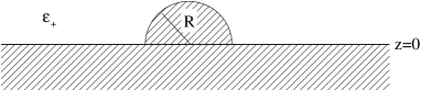
Figure 3: Domain of definition of the problem UP.

Problem UP in the domain $s>R$ and $z>0$, see Fig. 3:

$$\nabla^{2}\Phi_{+} = 0,\qquad{\mathbf{r}}\in\{s>R,z>0\},$$

$$\Phi_{+}(s=R,\theta,\varphi) = \Phi_{R}(\theta,\varphi),\qquad 0<\theta<\frac{\pi}{2},$$

$$\Phi_{+}(r,\varphi,z=0) = F_{0}(r,\varphi),\qquad r>R,$$

$$|\Phi_{+}({\mathbf{r}})| < \infty,\qquad|{\mathbf{r}}|\to\infty.$$

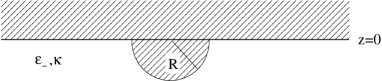
Figure 4: Domain of definition of the problem LOW.

Problem LOW in the domain $s>R$ and $z<0$, see Fig. 4:

$$\nabla^{2}\Phi_{-} = \kappa^{2}\Phi_{-},\qquad{\mathbf{r}}\in\{s>R,z<0\},$$

$$\Phi_{-}(s=R,\theta,\varphi) = \Phi_{R}(\theta,\varphi),\qquad\frac{\pi}{2}<\theta<\pi,$$

$$\Phi_{-}(r,\varphi,z=0) = F_{0}(r,\varphi),\qquad r>R,$$

$$|\Phi_{-}({\mathbf{r}})| < \infty,\qquad|{\mathbf{r}}|\to\infty.$$

Here $F_{0}(r,\varphi)$ (=potential at the interface $z=0$) is an auxiliary function which will be eventually determined by the boundary condition (4). Each of these problems can in turn be decomposed in simpler problems, one with boundary conditions imposed only at the plane $z=0$ and one with boundary conditions imposed only at the ball $s=R$:

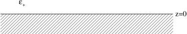
Figure 5: Domain of definition of the problem UP-cyl.

Problem UP-cyl in the domain $z>0$, see Fig. 5:

$$\nabla^{2}\Phi_{+}^{\rm cyl} = 0,\qquad{\mathbf{r}}\in\{z>0\},$$

$$\Phi_{+}^{\rm cyl}(r,\varphi,z=0) = F_{0}(r,\varphi)+{\cal F}_{0}(r,\varphi),\qquad 0<r,$$

$$|\Phi_{+}^{\rm cyl}({\mathbf{r}})| < \infty,\qquad|{\mathbf{r}}|\to\infty.$$

Figure 6: Domain of definition of the problem UP-sph.

Problem UP-sph in the domain $s>R$, see Fig. 6:

$$\nabla^{2}\Phi_{+}^{\rm sph} = 0,\qquad{\mathbf{r}}\in\{s>R\},$$

$$\Phi_{+}^{\rm sph}(R,\theta,\varphi) = \Phi_{R}(\theta,\varphi)-\Phi_{+}^{\rm cyl}(R,\theta,\varphi),\quad 0<\theta<\frac{\pi}{2},$$

$$\Phi_{+}^{\rm sph}(R,\theta,\varphi) = \mbox{}-\Phi_{+}^{\rm sph}(R,\pi-\theta,\varphi),\qquad\frac{\pi}{2}<\theta<\pi,$$

$$|\Phi_{+}^{\rm sph}({\mathbf{r}})| < \infty,\qquad|{\mathbf{r}}|\to\infty.$$

Here the function ${\cal F}_{0}(r,\varphi)$ verifies ${\cal F}_{0}(r>R,\varphi)=0$ and is an otherwise arbitrary smooth function which continues the potential $F_{0}(r,\varphi)$ into the region $r<R$ of the plane $z=0$. As discussed in the main text, ${\cal F}_{0}(r,\varphi)$ is just an intermediary auxiliary function whose precise choice is ultimately irrelevant for the determination of the total potential outside the ball $s=R$. With the choice of boundary condition for $\Phi_{+}^{\rm sph}$ at $s=R$ it is clear that $\Phi_{+}^{\rm sph}=0$ at $z=0$ and therefore

$$\Phi_{+}({\mathbf{r}})=\Phi_{+}^{\rm cyl}+\Phi_{+}^{\rm sph},\qquad{\rm if}\quad{\mathbf{r}}\in\{s>R,z>0\}.$$

Analogously, the problem LOW can be decomposed into a problem LOW-cyl and a problem LOW-sph and

$$\Phi_{-}({\mathbf{r}})=\Phi_{-}^{\rm cyl}+\Phi_{-}^{\rm sph},\qquad{\rm if}\quad{\mathbf{r}}\in\{s>R,z<0\}.$$

Each of these simpler problems is now amenable to an analytical solution, provided by Eqs. (II.2)–(7). The auxiliary functions $F_{0}$ and ${\cal F}_{0}$ are absorbed in the unknown coefficients $A_{m}(q)$ in Eq. (II.2), which are then determined by Eq. (4), the only boundary condition of the original problem not taken into account by the stepwise process of decomposing the problem into simpler ones.

References

- (1) F. H. Stillinger Jr., J. Chem. Phys. 35, 1584 (1961).
- (2) A. Hurd, J. Phys. A 18, L1055 (1985).
- (3) R. Aveyard et al., Langmuir 16, 1969 (2000).
- (4) O. Gómez-Guzmán and J. Ruiz-García, J. Colloid Interface Sci. 291, 1 (2005).
- (5) W. Chen, S. Tan, T.-K. Ng, W. T. Ford, and P. Tong, Phys. Rev. Lett. 95, 218301 (2005).
- (6) W. Chen, S. Tan, T.-K. Ng, W. T. Ford, and P. Tong, Phys. Rev. E 74, 021406 (2006).
- (7) J. C. Fernández–Toledano, A. Moncho–Jordá, F. Martínez–López, and R. Hidalgo–Alvarez, Langmuir 20, 6977 (2004).
- (8) L. Foret and A. Würger, Phys. Rev. Lett. 92, 058302 (2004).
- (9) M. Oettel, A. Domínguez, and S. Dietrich, Phys. Rev. E 71, 051401 (2005).
- (10) M. Oettel, A. Domínguez, and S. Dietrich, J. Phys.: Condens. Matter 17, L337 (2005).
- (11) A. Würger and L. Foret, J. Phys. Chem. B 109 16435 (2005).
- (12) A. Domínguez, M. Oettel, and S. Dietrich J. Chem. Phys., in press (2007).
- (13) K. A. Sharp and B. Honig, J. Phys. Chem 94, 7684 (1990).
- (14) Y. Zhou and T.-K. Ng, arXiv:cond-mat/0703667.
- (15) T.-K. Ng and Y. Zhou, arXiv:0708.2518.
- (16) E. Trizac and J.-L. Raimbault, Phys. Rev. E 60, 6530 (1999).