TMC-1C: an accreting starless core

Abstract

We have mapped the starless core TMC-1C in a variety of molecular lines with the IRAM 30m telescope. High density tracers show clear signs of self-absorption and sub-sonic infall asymmetries are present in ${\rm N}_{2}{\rm H}^{+}$(1–0) and ${\rm DCO}^{+}$(2–1) lines. The inward velocity profile in ${\rm N}_{2}{\rm H}^{+}$(1–0) is extended over a region of about 7,000 AU in radius around the dust continuum peak, which is the most extended “infalling” region observed in a starless core with this tracer. The kinetic temperature ($\sim 12$ K) measured from ${\rm C}^{17}{\rm O}$ and ${\rm C}^{18}{\rm O}$ suggests that their emission comes from a shell outside the colder interior traced by the mm continuum dust. The ${\rm C}^{18}{\rm O}$(2–1) excitation temperature drops from 12 K to $\simeq$10 K away from the center. This is consistent with a volume density drop of the gas traced by the ${\rm C}^{18}{\rm O}$ lines, from $\simeq$4$\times$10⁴ $\hbox{{\rm cm}}^{-3}$ towards the dust peak to $\simeq$6$\times$10³ $\hbox{{\rm cm}}^{-3}$ at a projected distance from the dust peak of 80″ (or 11,000 AU). The column density implied by the gas and dust show similar N₂H⁺ and CO depletion factors ($f_{D}\leq 6$). This can be explained with a simple scenario in which: (i) the TMC–1C core is embedded in a relatively dense environment ($n(\hbox{${\rm H}_{2}$})$ $\simeq$ 10⁴ $\hbox{{\rm cm}}^{-3}$), where CO is mostly in the gas phase and the ${\rm N}_{2}{\rm H}^{+}$ abundance had time to reach equilibrium values; (ii) the surrounding material (rich in CO and ${\rm N}_{2}{\rm H}^{+}$) is accreting onto the dense core nucleus; (iii) TMC-1C is older than 3$\times 10^{5}$ yr, to account for the observed abundance of ${\rm N}_{2}{\rm H}^{+}$ across the core ($\simeq$10^-10 w.r.t. ${\rm H}_{2}$); and (iv) the core nucleus is either much younger ($\simeq$ 10⁴ yr) or “undepleted” material from the surrounding envelope has fallen towards it in the past 10,000 yr.

1. Introduction

Dense starless cores in nearby low-mass star-forming regions such as Taurus represent the simplest areas in which to study the initial conditions of star formation. The dominant component of starless cores, H₂, is largely invisible in the quiescent interstellar medium, so astronomers typically rely on spectral line maps of trace molecules and continuum observations of the thermal emission from dust to derive their kinematics and physical state. However, it is now well established that different species and transitions trace different regions of dense cores, so that a comprehensive multi–line observations, together with detailed millimeter and sub–millimeter continuum mapping are required to understand the structure and the evolutionary status of an object which will eventually form a protostar and a protoplanetary system.

Previous studies of starless cores in Taurus, as well as other nearby star-forming regions, have shown that the relative abundance of many molecules varies significantly between the warmer, less dense envelopes and the colder, denser interiors (see Ceccarelli et al. 2006 and Di Francesco et al. 2006 for detailed reviews on this topic). For instance, Caselli et al. (1999), Bergin et al. (2002) and Tafalla et al. (2004) have shown that carbon-bearing species such as C¹⁷O, C¹⁸O, C³⁴S, and CS are largely absent from the cores L1544, L1498 and L1517B at densities larger than a few 10⁴ cm^-3, while nitrogen-bearing species such as N₂H⁺ and ammonia are preferentially seen at high densities. The chemical variations within a starless core are likely the result of molecular freeze–out onto the surfaces of dust grains at high densities and low temperatures, followed by gas phase chemical processes, which are profoundly affected by the abundance drop of important species, in particular CO (see e.g. Dalgarno & Lepp, 1984; Bergin & Langer, 1997; Taylor et al., 1998; Aikawa et al., 2005).

In the past few years it has also been found that not all starless cores show a similar pattern of molecular abundances and physical structure. Indeed, there is a subsample of starless cores (often called pre-stellar cores), which are particularly centrally concentrated, that shows kinematic and chemical features typical of evolved objects on the verge of star formation. These features include large values of CO depletion and deuterium fractionation, and evidence of “central” infall, i.e. presence of infall asymmetry in high density tracers in a restricted region surrounding the mm continuum dust peak (Williams et al., 1999; Caselli et al., 2002a; Redman et al., 2002; Crapsi et al., 2005; Williams et al., 2006). It is interesting that not all physically evolved cores show chemically evolved compositions, as shown by Lee et al. (2003) and Tafalla & Santiago (2004b). It is thus important to study in detail a larger number of cores to understand what is causing the chemical differentiation in objects with apparently similar physical ages. This is why we decided to focus our attention on TMC–1C, a dense core in Taurus, with physical properties quite similar to the prototypical pre–stellar core L1544 (also in Taurus), to study possible differences and try to understand their nature.

TMC–1C is a starless core in the Taurus molecular cloud, with a distance estimated at 140 pc (Kenyon et al., 1994). In a previous study, we have shown that TMC–1C has a mass of 6 M_⊙ within a radius of 0.06 pc from the column density peak, which is a factor of two larger than the virial mass derived from the N₂H⁺(1–0) line width, and we have shown that there is evidence for sub-sonic inward motions (Schnee & Goodman, 2005) as well as a velocity gradient consistent with solid body rotation at a rate of 0.3 km s^-1 pc^-1 (Goodman et al., 1993). TMC–1C is a coherent core with a roughly constant velocity dispersion, slightly higher than the sound speed, over a radius of 0.1 pc (Barranco & Goodman, 1998; Goodman et al., 1998). Using SCUBA and MAMBO bolometer maps of TMC-1C at 450, 850 and 1200 µm, we have mapped the dust temperature and column density and shown that the dust temperature at the center of the core is very low ($\sim$6 K) (Schnee et al., 2007).

In order to disentangle the physical and chemical information that can be gleaned from a combination of gas and dust observations of a dense core, we have now mapped TMC-1C at three continuum wavelengths (Schnee et al., 2007) and seven molecular lines. In Sec. 2, continuum and line observations are described. Spectra and maps are presented in Sec. 3. The analysis of the data, along with the discussion, has been divided in three parts: kinematics, including line width variations across the cloud, velocity gradients and inward velocities, is in Sec. 4; gas and dust column density and temperature are in Sect. 5; molecular depletion and chemical processes are discussed in Sect. 6. A summary can be found in Sect. 7.

2. Observations

2.1. Continuum

To map the density and temperature structure of TMC–1C, we have observed thermal dust emission at 450 and 850 µm with SCUBA and at 1200 µm with MAMBO–2.

2.1.1 SCUBA

We observed a 10′$\times$10′ region around TMC-1C using SCUBA (Holland et al., 1999) on the JCMT at 450 and 850 µm. We used the standard scan-mapping mode, recording 450 and 850 µm data simultaneously (Pierce-Price et al., 2000; Bianchi et al., 2000). Chop throws of 30″, 44″ and 68″ were used in both the right ascension and declination directions. The resolution at 450 and 850 µm is 7.5″ and 14″ respectively. The absolute flux calibration is $\sim$12% at 450 µm and $\sim$4% at 850 µm. The noise in the 450 and 850 µm maps are 13 and 9 mJy/beam, respectively. The data reduction is described in detail in Schnee et al. (2007).

2.1.2 MAMBO-2

Kauffmann et al. (in prep.) used the MAMBO-2 array (Kreysa et al., 1999) on the IRAM 30–meter telescope on Pico Veleta (Spain) to map TMC–1C at 1200 µm. The MAMBO beam size is 10$\farcs$7. The source was mapped on-the-fly, chopping in azimuth by 60″ to 70″ at a rate of 2 Hz. The absolute flux calibration is uncertain to $\sim$10%, and the noise in the 1200 µm map is 3 mJy/beam. The data reduction is described in detail in Kauffmann et al. (in prep.).

2.2. Spectral Line

We have used the IRAM 30-m telescope to map out emission from several spectral lines in order to understand the kinematic and spectral structure of TMC–1C. In November 1998, we mapped the spectral line maps of the C¹⁷O(1–0), C¹⁷O(2–1), C¹⁸O(2–1), C³⁴S(2–1), DCO⁺(2–1), DCO⁺(3–2), N₂H⁺(1–0) transitions. The inner 2′ of TMC-1C were observed with 20″ spacing in frequency-switching mode, and outside of this radius the data were collected with 40″ sampling. The data were reduced using the CLASS package, with second-order polynomial baselines subtracted from the spectra. The system temperatures, velocity resolution, beam size and beam efficiencies are listed in Table 1.

3. Results

3.1. Spectra

The spectra taken at the peak of the dust column density map are shown in Figure 1. The integrated intensity, velocity, line width and RMS noise for each transition is given in Table 2. From the figure it is evident that self–absorption is present everywhere, except in ${\rm C}^{17}{\rm O}$ and ${\rm C}^{18}{\rm O}$ lines. Clear signatures of inward motions (brighter blue peak; e.g. Myers et al. 1997, see also Sect. 4.3) are only present in the high density tracers ${\rm N}_{2}{\rm H}^{+}$and ${\rm DCO}^{+}$, which typically probe the inner portion of dense cores (e.g. Caselli et al. 2002b; Lee et al. 2004). The C³⁴S(2–1) line appears to be self–absorbed at the cloud velocity, but the spectrum is too noisy to confirm this.

To highlight the extent of the “infall” asymmetry in ${\rm N}_{2}{\rm H}^{+}$(1–0), Fig. 2 shows the profile of the main hyperfine component of the ${\rm N}_{2}{\rm H}^{+}$(1–0) transition (F₁,F = 2,3 $\rightarrow$ 1,2) across the whole mapped area (see Sect. 3.2). We will discuss these spectra in more detail in Sect. 4.3, but for now it is interesting to see how the profile shows complex structure, consistent with inward motion (red boxes) as well as outflow (blue boxes) and absorption from a static envelope.

3.2. Maps

From Fig. 1 and 2, it is clear that the main ${\rm N}_{2}{\rm H}^{+}$(1–0) hyperfine components are self-absorbed around the dust peak position. Therefore, a map of the ${\rm N}_{2}{\rm H}^{+}$(1–0) intensity integrated under the seven components will not reflect the ${\rm N}_{2}{\rm H}^{+}$ column density distribution. However, the weakest component (F₁ F = 10 $\rightarrow$ 11) is not affected by self-absorption, as shown in Fig. 3, where the weakest and the main (F₁ F = 23 $\rightarrow$ 12) components toward the dust peak position (the most affected by self-absorption) are plotted together for comparison. The two hyperfines in Fig. 3 have very different profiles: the main component is blue-shifted, suggestive of inward motions (see Sect. 4.3), whereas the weak component is symmetric and its velocity centroid is red shifted compared to the main component, indicating optically thin emission. Given that the self-absorption is more pronounced at the position of the dust peak, where the ${\rm N}_{2}{\rm H}^{+}$(1–0) optical depth is largest, we conclude that the weak component is likely to be optically thin across the whole TMC–1C core.

Thus, in the case of ${\rm N}_{2}{\rm H}^{+}$(1–0) self–absorption, we used the weak hyperfine component, divided by 1/27 (its relative intensity compared to the sum, normalized to unity, of the seven hyperfines), to determine the ${\rm N}_{2}{\rm H}^{+}$(1–0) integrated intensity, line width, and, as shown in Sec. 5, the ${\rm N}_{2}{\rm H}^{+}$ column density. In this analysis, only spectra with signal to noise (S/N) for the weak component $>$ 3 have been considered. In all other cases, ${\rm N}_{2}{\rm H}^{+}$(1–0) did not show signs of self–absorption and a normal integration below the 7 hyperfines has been performed.

Based on hyperfine fits to the C¹⁷O(1–0) transition and a comparison of the relative strengths of the three components, we see that the C¹⁷O(1–0) emission is optically thin throughout TMC–1C. Although the noise is generally too high in the C¹⁷O(2–1) data to make indisputable hyperfine fits, the results of such an attempt suggest that the C¹⁷O(2–1) lines are also optically thin, which is expected for thin C¹⁷O(1–0) emission and temperatures of $\sim$10 K. Thus, the integrated intensity maps of ${\rm C}^{17}{\rm O}$ lines will reflect the ${\rm C}^{17}{\rm O}$ column density distribution.

In order to estimate the optical depth of the C¹⁸O(2–1) lines, we compare the integrated intensity of C¹⁸O(2–1) to that of C¹⁷O(2–1). If both lines are thin, then the observed ratio should be equal to the cosmic abundance ratio, $R_{18,17}\equiv$ [¹⁸O]/[¹⁷O] = 3.65 (Wilson & Rood, 1994; Penzias, 1981). We observe that the ratio of the integrated intensities $R_{18,17}=2.3\pm 0.9$, which corresponds to an optical depth of the C¹⁸O(2–1) line of $\tau_{18}\simeq 1.5$.

Integrated intensity maps of C¹⁷O(1–0), C¹⁷O(2–1), C¹⁸O(2–1), DCO⁺(2–1) and N₂H⁺(1–0) are shown in Fig. 4. Note that the N₂H⁺ integrated intensity map peaks right around the position of the dust column peaks, which is not true for C¹⁷O and C¹⁸O. We do not present integrated intensity maps of C³⁴S(2–1) or DCO⁺(3–2), which have lower signal to noise.

4. Analysis. I. Kinematics

4.1. Line Widths

Ammonia observations have shown that TMC–1C is a coherent core, having a constant line width across the core at a value slightly higher than the thermal width, and increasing outside the “coherent” radius, $\sim$0.1 pc (Barranco & Goodman, 1998). Our N₂H⁺ observations of TMC–1C show that the line width remains constant, at a value $\sim$2 times higher than the thermal line width, over the entire core (see Fig. 5 for a map of the line width and a plot of line width vs. radius), though the dispersion in the N₂H⁺ line width is very large. This result is in agreement with the NH₃ observations of TMC–1C, and is not consistent with the decreasing N₂H⁺ and N₂D⁺ linewidths at larger radii seen in L1544 and L694-2, which in other important ways (density and temperature structure, velocity asymmetry seen in ${\rm N}_{2}{\rm H}^{+}$(1–0)) closely resemble TMC–1C. To make sure that the lack of correlation of the ${\rm N}_{2}{\rm H}^{+}$(1–0) line width is not due to geometric effects, considering the elongated structure of TMC–1C, we also plotted the ${\rm N}_{2}{\rm H}^{+}$(1–0) line width as a function of antenna temperature, and found similar results.

This behavior may be due to the coherence of the central portion of the core, which has nearly constant length along the line of sight, and thus the velocity dispersion comes from regions of the core that have similar scales (see Fig. 4 in Goodman et al. 1998). Cores formed by compressions in a supersonic turbulent flow naturally develop these regions of constant length at their centers (Klessen et al., 2005). Another reason that the N₂H⁺ line widths appear constant across the cloud could be the different “infall” velocity profile, with the velocity peaking farther away from the dust peak than in L1544 and L694-2 (though the projected velocity would still be at its maximum at the dust peak). In the case of L1544, Caselli et al. (2002a) showed that the ${\rm N}_{2}{\rm H}^{+}$(1–0) line profile is consistent with the Ciolek & Basu (2000) model at a certain time in the cloud evolution, where the “infall” velocity profile peaks at a radius of about 3,000 AU (see also Myers 2005 for alternative models with similar radial velocities). Indeed, in Sec. 4.3 we show that the extent of the asymmetry seen in ${\rm N}_{2}{\rm H}^{+}$(1–0) suggests that the peak of the inward motions is at about 7,000 AU, so that one does not expect to see broader line widths within this radius. In fact, the binned data in Fig. 5 show a hint of a peak at about 50″ (7000 AU at the distance of Taurus).

In order to compare the thermal and non-thermal line widths in TMC-1C, we assume that the gas temperature is equal to 10 K and use the formulae:

$$\Delta v_{T}=\sqrt{\left(\frac{8\ln(2)\,kT_{g}}{\mu m_{H}}\right)}$$ (1)

$$\Delta v_{NT}=\sqrt{(\Delta v_{obs})^{2}-(\Delta v_{T})^{2}}$$ (2)

where $\mu$ is the molecular weight of the species and $m_{H}$ is the mass of hydrogen.

Figure 6 shows the non-thermal line width plotted against the thermal line width at the position of the dust column density peak. To allow a fair comparison, all the data in the figure have been first spatially smoothed at the same resolution of the ${\rm NH}_{3}$ map (1′). Although C¹⁷O, C¹⁸O, DCO⁺ and N₂H⁺ all have similar molecular weights, they have significantly different values for their non-thermal line widths. The thermal line width is much smaller than the non-thermal line width for the molecules C¹⁷O and C¹⁸O, while the ratio is closer to unity for DCO⁺ and N₂H⁺. This suggests that the isotopologues of CO are tracing material at larger distances from the center, with a larger turbulent line width, than are DCO⁺ and N₂H⁺, which presumably are tracing the higher density material closer to the center of TMC-1C. The C¹⁸O(2–1) line is slightly thick, and this is probably the reason of its slightly larger line width when compared to the thin C¹⁷O(2–1) line, as shown in Figure 6. For each transition observed, we see no clear correlation between the observed line width and the thermal line width (and therefore with temperature, column density and distance from the peak column density, see Section 5.2). As in the study of depletion, the lower signal to noise in C³⁴S(2–1), DCO⁺(2–1) and DCO⁺(3–2) make any possible trends between $\Delta v$ and $\Delta v_{thermal}$ more difficult to determine. From Fig. 6 we note that NH₃ and N₂H⁺ have similar non-thermal line widths, which makes sense given that ${\rm N}_{2}{\rm H}^{+}$ and ${\rm NH}_{3}$ are expected to trace similar material (e.g. Benson et al. 1998). However, this result is in contrast with the findings of Tafalla et al. (2004) who found narrower ${\rm NH}_{3}$ line widths towards L1498 and L1517B.

We finally note that the line widths that we measure in C¹⁷O and C¹⁸O are larger than the N₂H⁺ linewidths throughout TMC–1C, which contrasts with the results seen in C¹⁸O and N₂H⁺ in B68 (Lada et al., 2003). This is consistent with the fact that TMC–1C, unlike B68, is embedded in a molecular cloud complex and it is not an isolated core. Thus, CO lines in TMC–1C also trace the (lower density and more extended) molecular material, part of the Taurus complex, where larger ranges of velocities are present along the line of sight.

4.2. Velocity Gradients

In order to study the velocity field of TMC-1C, we determine the centroid velocities for C¹⁷O(2–1), C¹⁸O(2–1), C³⁴S(2–1), DCO⁺(2–1) and DCO⁺(3–2) with Gaussian fits. The centroid velocities of the C¹⁷O(1—0) and N₂H⁺(1–0) lines are determined by hyperfine spectral fits. For those N₂H⁺ spectra that show evidence of self-absorption, the velocity is derived from a Gaussian fit to the thinnest component. The velocity gradient at each position is calculated by fitting the velocity field with the function:

$$v_{lsr}=v_{o}+\frac{dv}{ds}\Delta\alpha\cos{\theta}+\frac{dv}{ds}\Delta\delta\sin{\theta}$$ (3)

where $v_{o}$ is the bulk motion along the line of sight, $\Delta\alpha$ and $\Delta\delta$ are RA and DEC offsets from the position of the central pixel, $dv/ds$ is the magnitude of the velocity gradient in the plane of the sky, and $\theta$ is direction of the velocity gradient. The fit to the velocity gradient is based on fitting a plane through the position–position velocity cube as in Goodman et al. (1993) (for the “total” gradient across the cloud) and in Caselli et al. (2002b) (for the “local” gradient at each position). The fit for the “total” velocity gradient gives a single direction and magnitude for the entire velocity field analyzed. The “local” velocity gradient is calculated at each position in the spectral line maps based on the centroid velocities of the center position and its nearest neighbors, with the weight given to the neighbors decreasing exponentially with their distance from the central position.

Analysis of ammonia observations with $\sim 60$″ resolution of TMC–1C indicate an overall velocity gradient of 0.3 km s^-1 pc^-1 directed 129 degrees East of North (Goodman et al., 1993). The velocity field that we measure in TMC–1C has spatial resolution three times greater ($\sim$20″) than the ammonia study, and reveals a pattern more complicated than that of solid body or differential rotation. The velocity fields measured by C¹⁷O(1–0), C¹⁷O(2–1) and C¹⁸O(2–1) are shown in Fig. 7. Although there is a region that closely resembles the velocity field expected from rotation (gradient arrows of approximately equal length pointing in the same direction), the measured velocities vary from blue to red to blue along a NW - SE axis. The N₂H⁺(1–0) velocity fields (shown in Fig. 7) also follow the same blue to red to blue pattern along the NW - SE axis, but the observations cover a somewhat different area than the CO observations, which complicates making a direct comparison. Taken as a whole, it is clear that there is an ordered velocity field in portions of the TMC-1C core, and that the lower density CO tracers “see” a velocity field similar to that probed by N₂H⁺ lines, which trace higher density material. In any case, the velocity field that looks like rotation reported in Goodman et al. (1993) turns out to be more complicated when seen over a larger area with finer resolution. The direction and magnitude of the velocity gradient in the region that resembles solid body rotation is shown in Fig. 8 for each transition.

4.3. Inward Motions

To quantify the velocity of the inward motion from the ${\rm N}_{2}{\rm H}^{+}$(1–0) line across the TMC–1C cloud, we use a simple two–layer model, similar to that described by Myers et al. (1996). This model assumes that the cloud can be divided in two parts with uniform excitation temperature ($T_{\rm ex}$, gradients in $T_{\rm ex}$ between the two layers as in De Vries & Myers 2005, are not considered here), line width ($\Delta v$), optical depth ($\tau$) and LSR velocity ($V_{\rm LSR}$) and that the foreground layer has a lower excitation temperature. For simplicity, we also assume that the seven hyperfines have the same $T_{\rm ex}$, which is a very rough assumption in regions of large optical depth, as recently found by Daniel et al. (2006). Despite of the simplicity of the model, we find good fits to the seven hyperfine lines and determine the value of the velocity difference between the two layers, which can be related to the “infall” velocity.

In Fig. 9 we present five spectra which represent a cut across the major axis of the core, passing through the dust peak. For display purposes, the spectra have been centered to 0 velocity, subtracting the LSR velocity obtained from a Gaussian fit to the weak hyperfine component (for offsets [-40,60], [-20,40], [0,20], where the self-absorption in present) or hfs fits in CLASS (for offsets [20,0] and [40,-20]). The $V_{\rm LSR}$ velocity is shown in the top right of each panel. The cut is from South-East (offset [40,-20], see Fig. 2) to North-West (offset [-40,60]). The first thing to note in the figure is that clear signs of self-absorption and asymmetry are present toward the dust peak and in the North-West, but not in the two Southern positions. This trend can also be seen as a general feature in Fig. 2, where it is evident that asymmetric lines are more numerous North–West of the dust peak.

The excitation temperature, total optical depth, line width and the velocity ($V-V_{\rm LSR}$, see Fig. 9) of the foreground (F) and background (B) layers are reported in Table 3. To find the best fit parameters, we first performed an hfs fit to the [20,0] spectrum, which is the closest spectrum to the dust peak not showing self-absorption. The values of $\tau_{\rm TOT}$, $T_{\rm ex}$ and line width obtained from this fit have been adopted for the background emission at the dust peak position and the best fit has been found by adding the foreground layer and minimising the residuals. For the two spectra North–West of the [0,20] position, adjustment to the parameters of the background layer were necessary to obtain a good fit. We point out that the five spectra we chose for this analysis are representative of the whole area surrounding the TMC–1C dust peak, where a mixture of symmetric, blue–shifted and red–shifted spectra are present. As already stated, the majority of the asymmetric spectra show inward motions and extend over a region with radius $\sim$7000 AU (see Fig. 2).

The properties derived for the foreground layer ($T_{\rm ex}$ $\simeq$3.3–3.5 K, $\tau_{\rm TOT}$ $\simeq$10–15, and $\Delta v\simeq$0.2 ${\rm km\,s}^{-1}$) have been used as input parameters in a Large Velocity Gradient (LVG) code for a uniform medium and found to be consistent with the ${\rm N}_{2}{\rm H}^{+}$(1–0) tracing gas at a density $n(\hbox{${\rm H}_{2}$})$ $\simeq$ 5$\times$10³ $\hbox{{\rm cm}}^{-3}$, kinetic temperature $T_{\rm kin}$ $\simeq$ 10 K and with column density $N(\hbox{${\rm N}_{2}{\rm H}^{+}$})$ $\simeq$ 5$\times$10¹² $\hbox{{\rm cm}}^{-2}$, values comparable to those found for the background layer (see Table 5 and Sec. 5.1).

It is interesting that the maximum of the line-of-sight component of the inward velocity ($\sim$0.15 ${\rm km\,s}^{-1}$) is found toward the dust peak, whereas one pixel away from it, the inward velocity drops to 0.05 ${\rm km\,s}^{-1}$. This is suggestive of a geometric effect, in which the inward velocity vector is directed toward the dust peak, so that only a fraction $cos(\theta)$ (with $\theta$ the angle between the l.o.s. and the infall velocity direction) of the total velocity is directed along the line of sight in those positions away from the dust peak. Of course, our simplistic model prevents us to go further than this, i.e. the uncertainties are too large to build a 3D model of the velocity profile within the cloud.

As shown in Fig. 2, in the North–West end of the TMC–1C core (around offset [-250,150]), there are other signatures of inward motions, which may indicate the presence of another gravitational potential well. This suggestion is indeed reinforced by Fig. 8 of Schnee et al. (2007), which shows high extinction and low temperatures in the same direction. Unfortunately, the continuum coverage is not good enough to attempt a detailed analysis, but it appears evident that the extension toward the North–West is another dense core connected to the main TMC–1C condensation with lower density and warmer gas and dust.

5. Analysis. II. Column Density and Temperature

5.1. Gas Column Density

To derive the column density of gas from each molecule, we assume that all rotation levels are characterized by the same excitation temperature $T_{ex}$ (the CTEX method, described in Caselli et al. 2002b). In case of optically thin emission,

$$N_{tot}=\frac{8\pi W}{\lambda^{3}A}\frac{g_{l}}{g_{u}}\frac{1}{J_{\nu}(T_{ex})-J_{\nu}(T_{bg})}\frac{1}{1-\exp(-h\nu/kT_{ex})}\frac{Q_{rot}}{g_{l}\exp(-E_{l}/kT_{ex})}$$ (4)

where $\lambda$ and $\nu$ are the wavelength and frequency of the transition, $k$ is the Boltzmann constant, $h$ is the Planck constant, $A$ is the Einstein coefficient, $g_{l}$ and $g_{u}$ are the statistical weights of the lower and upper levels, $J_{\nu}(T_{ex})$ and $J_{\nu}(T_{bg})$ are the equivalent Rayleigh-Jeans excitation and background temperatures, W is the integrated intensity of the line. The partition function ($Q_{rot}$) and the energy of the lower level ($E_{l}$) for linear molecules are given by:

$$Q_{rot}=\sum_{J=0}^{\infty}(2J+1)\exp(-E_{J}/kT)$$ (5)

and

$$E_{J}=J(J+1)hB$$ (6)

and $B$ is the rotational constant (see Table 4 for the values of the constants).

The ${\rm C}^{17}{\rm O}$(1–0) and (2–1) lines have hyperfine structure, enabling the measurement of the optical depth. We find that the lines are optically thin throughout the core. To determine the column density, we assume an excitation temperature of 11 K, which is the average value of $T_{\rm ex}$ found from our ${\rm C}^{18}{\rm O}$ data around the dust peak position, as explained in Sect. 5.3. In the case of ${\rm C}^{18}{\rm O}$(2–1) lines, we correct for optical depth before determining the column density, using the correction factor:

$$C_{\tau} = \frac{\tau}{1-e^{-{\tau}}}$$ (7)

As explained in Sect. 3.1, ${\rm N}_{2}{\rm H}^{+}$(1–0) lines show clear signs of self–absorption in an extended area around the dust peak. To determine the column density across the core, first we select spectra without self–absorption, and those with high S/N (i.e. with $W/\sigma_{W}$ $>$ 20, with $W$ $\equiv$ integrated intensity; see Caselli et al. 2002b) have been fitted in CLASS to find $T_{\rm ex}$ and $\tau$. The mean value of $T_{\rm ex}$ found with this analysis (4.4$\pm$0.1 K) has been used for all other positions where an independent estimate of $T_{\rm ex}$ was not possible (i.e. for self-absorbed or thin lines). For optically thin ${\rm N}_{2}{\rm H}^{+}$(1–0) transitions, the intensity was integrated below the seven hyperfine and the expression (4) used to determine the total column density.

In cases of self-absorbed spectra, the ${\rm N}_{2}{\rm H}^{+}$ column density has been estimated from the integrated intensity of the weakest (and lowest frequency) hyperfine component ($F_{1}F$ = 1 0$\rightarrow$1 1), using eq. 4 (assuming $T_{\rm ex}$=4.4 K) and multiplying by 27 (the inverse of the hyperfine relative intensity). The weakest component is not affected by self–absorption, as shown in Fig. 3, suggesting that its optical depth is low. We have checked that these two different methods approximately give the same results by measuring the ${\rm N}_{2}{\rm H}^{+}$ column density with both procedures in those cases where self-absorption is not present and where the weakest hyperfine component has a S/N ratio of at least 4. We found that the two column density values agree to within 10%.

${\rm DCO}^{+}$(2–1) and ${\rm DCO}^{+}$(3–2) lines are clearly self–absorbed and the column density determination is very uncertain (given that there are no clues about their optical depth and excitation temperature). The estimates listed in Table 5 should be considered lower limits. $T_{\rm ex}$ = 4.4 K has beed assumed, based on the fact that the ${\rm DCO}^{+}$ lines are expected to trace similar conditions than ${\rm N}_{2}{\rm H}^{+}$. C³⁴S(2–1) spectra have low sensitivity, and the lines are affected by self–absorption (see Fig. 1), so the derived C³⁴S column density is highly uncertain.

The ${\rm N}_{2}{\rm H}^{+}$ abundance, $X(\hbox{${\rm N}_{2}{\rm H}^{+}$})$ ($\equiv$ $N(\hbox{${\rm N}_{2}{\rm H}^{+}$})/N(\hbox{${\rm H}_{2}$})$), toward the dust peak is 1.6$\times$10^-10, identical (within the errors) to that derived toward the L1544 dust peak (Crapsi et al., 2005, e.g.). This is interesting considering that $N(\hbox{${\rm H}_{2}$})$ in TMC–1C is 1.6 times lower than in L1544, in which ${\rm N}_{2}{\rm H}^{+}$ closely follows the dust column (as already found in previous work). However, unlike L1544, where the ${\rm N}_{2}{\rm H}^{+}$ abundance appears constant with impact parameters (e.g. Tafalla et al. 2002 and Vastel et al. 2006), in TMC–1C the ${\rm N}_{2}{\rm H}^{+}$ abundance increases away from the dust peak by a factor of about two within 50″, as shown in Fig. 10 (see also Fig. 14 in Sect. 6.1). Fig. 10 displays $A_{\rm V}$ (see Sect. 5.2), $N(\hbox{${\rm N}_{2}{\rm H}^{+}$})$ and $X(\hbox{${\rm N}_{2}{\rm H}^{+}$})$, normalized to the corresponding maximum values (63.2 mag, 1.1$\times$10¹³ $\hbox{{\rm cm}}^{-2}$, and 4.8$\times$10^-10, respectively) in two cuts (one in right ascension and one in declination) passing through the dust peak. One point to note is that the abundance derived at the dust peak (marked by the black dotted line) is the minimum value observed, indicating moderate (factor of $\sim$2) depletion.

5.2. Dust Column Density

In Schnee et al. (2007) we used SCUBA and MAMBO maps at 450, 850 and 1200 µm to create column density and dust temperature maps of TMC–1C. In this paper we smooth the dust continuum emission maps to the 20″ spacing of the IRAM maps and then derive $A_{\rm V}$ and $T_{d}$ to facilitate a direct comparison of the gas and dust properties. At each position, we make a non-linear least squares fit for the dust temperature and column density such that the difference between the predicted and observed 450, 850 and 1200 µm observations is minimized. The errors associated with such a fitting procedure are described in Schnee et al. (2007). Dust column density and temperature maps of TMC–1C are shown in Fig. 8 of Schnee et al. (2007).

From Fig. 8 in Schnee et al. (2007), it is clear that there is an anti-correlation between extinction and dust temperature (as also predicted by theory, e.g. Evans et al. 2001, Zucconi et al. 2001, Galli et al. 2002). To better show this, the two quantities are plotted in Fig. 11. The data in Fig. 11 are not smoothed to the IRAM 30m beam at 3 mm, since this is only a dust property intercomparison and does not refer to the gas properties. Higher $A_{\rm V}$ (60 $<A_{\rm V}\leq$ 90 mag) and lower dust temperatures (5 $\leq T_{\rm dust}<$ 6 K) are detectable at the higher resolution. We compare the $T_{\rm d}-A_{\rm V}$ relationship seen in TMC–1C with that predicted by Zucconi et al. (2001) for an externally heated pre-protostellar core (the solid red line in Fig. 11). We find that at high column density ($A_{\rm V}>30$) the observed dust temperature in TMC–1C is lower than that of the model core, while at low column density ($10<A_{\rm V}<20$) the observed dust temperature is higher than the model predicts. However, given that the model predicts the dust temperature at the center of a spherical cloud, and that the geometry of TMC–1C is certainly not spherical, only a rough agreement between the model and observations should be expected.

5.3. Gas Temperature

Because of its low dipole moment, CO is a good gas thermometer, given that it is easily thermalized at typical core densities. However, it is now well established that CO is significantly frozen onto dust grains at densities $\geq$ 10⁵ cm^-3 (one exception being L1521E; Tafalla & Santiago, 2004b) and this is also the case in TMC–1C. Therefore, at the dust peak we do not expect to measure a gas temperature from CO of $\sim$7 K, but instead a higher value reflecting the temperature in the outer layers of the cloud. The lines available for this analysis are: C¹⁷O(1–0), C¹⁷O(2–1), and C¹⁸O(2–1). The C¹⁷O(2–1)/C¹⁸O(2–1) brightness temperature ratio has been used to derive the excitation temperature of the C¹⁸O line, which is coincident with the kinetic temperature if the line is thermalized. To test the hyposthesis of thermalization we use an LVG (Large-Velocity-Gradient) program to determine at which volume density and kinetic temperature the observed C¹⁷O(1–0) and C¹⁷O(2–1) brightness temperatures can be reproduced. We use a one-dimensional non-LTE radiative transfer code (van der Tak et al., 2007) available at http://www.strw.leidenuniv.nl/ moldata/radex.html.

5.3.1 C¹⁷O(2-1) and C¹⁸O(2-1) as a measure of $T_{\rm kin}$

These two lines have similar frequencies, so the corresponding angular resolution is almost identical and no convolution is needed. Following a similar analysis done with the J=1–0 transition of the two CO isotopologues (Myers et al. 1983), the optical depth of the C¹⁸O(2–1) line ($\tau_{18}$) can be found from:

$$\frac{T_{\rm mb}[\hbox{${\rm C}^{18}{\rm O}$}(2-1)]}{T_{\rm mb}[\hbox{${\rm C}^{17}{\rm O}$}(2-1)]} = 3.65\times\frac{1-e^{-\tau_{18}}}{\tau_{18}},$$ (8)

where $T_{\rm mb}[i]$ is the main beam brightness temperature of transition $i$ (assuming a unity filling factor). The last term in the right hand side is the optical depth correction which is used to determine the total column density of ${\rm C}^{18}{\rm O}$ in a plane parallel geometry, which most likely applies to CO emitting regions, i.e. the external core layers.

Once $\tau_{18}$ is measured, the excitation temperature ($T_{\rm ex}$) of the corresponding transition (thus the gas kinetic temperature, if the line is in local thermodynamic equilibrium) can be estimated from the radiative transfer equation:

$$T_{\rm mb} = [J_{\nu}(T_{\rm ex})-J_{\nu}(T_{\rm bg})](1-e^{-\tau}),$$ (9)

where $J_{\nu}(T_{\rm ex})$ and $J_{\nu}(T_{\rm bg})$ are the equivalent Reyleigh–Jeans temperatures, with

$$J_{\nu}(T)=\frac{T_{0}}{\exp(T_{0}/T)-1},$$ (10)

$T_{0}$ = $h\nu/k_{\rm B}$, and $\nu$ the frequency of the ${\rm C}^{18}{\rm O}$(2–1) line (see Table 1).

Figure 12 (left panel) shows the results of this analysis. The set of data points in Fig. 12 is limited to only those spectra with $T_{\rm mb}[\hbox{${\rm C}^{17}{\rm O}$}(2--1)]/T_{\rm rms}$ $\geq$ 10, to avoid scatter due to noise. The error associated with the gas temperature has been calculated by propagating the errors on $\tau_{18}$ and $T_{\rm mb}$[${\rm C}^{18}{\rm O}$(2–1)] into Eq. 9 and its expression is given in the appendix.

It is interesting to note that the ${\rm C}^{18}{\rm O}$(2–1) excitation temperature appears to decrease away from the center, and, if this line is thermalized, it suggests that the kinetic temperature also drops away from the center, in contrast with the dust temperature. Indeed, the two quantities are completely uncorrelated in the 12 common positions with large S/N ${\rm C}^{18}{\rm O}$(2–1) spectra (not shown). $T_{\rm ex}$ is close to 12 K at the core center, whereas it drops to 9–10 K one arcmin away from the dust peak. Is this drop due to a decreasing gas temperature, as recently found by Bergin et al. (2006) in the Bok Globule B68? Unlike B68, we believe that our result is due to the volume density decrease. Indeed, the critical densities of the J = 2–1 lines of ${\rm C}^{17}{\rm O}$ and ${\rm C}^{18}{\rm O}$ are a few $\times$ 10⁴ $\hbox{{\rm cm}}^{-3}$, so that only if the volume density traced by one of the two isotopologues is larger than, say, 5$\times$10⁴ $\hbox{{\rm cm}}^{-3}$ can the J = 2–1 lines be considered good gas thermometers. In the next subsection, we investigate this point more quantitatively.

5.3.2 C¹⁷O(1–0) and C¹⁷O(2–1) to measure $T_{\rm ex}$[${\rm C}^{17}{\rm O}$(2–1)]

In Fig. 12 (right panel), the brightness temperature ratio of the ${\rm C}^{17}{\rm O}$(1–0) and ${\rm C}^{17}{\rm O}$(2–1) lines is plotted as a function of distance from the dust peak. Because of the different angular resolutions at the 2–1 and 1–0 frequencies, the 1 mm data have been smoothed to the 3 mm resolution and both data cubes have then been regridded, to allow a proper comparison. The ratio is indeed increasing towards the edge of the cloud, consistent with our previous finding of a $T_{\rm ex}$[${\rm C}^{18}{\rm O}$(2–1)] drop in the same direction (see left panel).

Both ${\rm C}^{17}{\rm O}$(1–0) and (2–1) lines possess hyperfine structure, which provides a direct estimate of the line optical depth. Using the hfs fit procedure available in CLASS, we found that all over the TMC–1C cloud, both lines are optically thin. This means that it is not possible to derive the excitation temperature in an analytic way, so we use the LVG code introduced in Sect. 5.3. This code assumes homogeneous conditions, which is likely to be a good approximation for the region traced by CO isotopologues. In fact, because of freeze-out, CO does not trace the regions with densities larger than about 10⁵ cm^-3 (see below and Sect. 6.1), so that the physical conditions traced by CO around the dust peak are likely to be close to uniform (n(H₂) $\sim$ a few times 10⁴ and about constant temperature). This is also supported by the integrated intensity CO maps, which appear extended and uniform around the dust peak (see Fig. 4).

To better understand this result, the LVG code has been run to see how changes in volume density and gas temperature affect the line ratio. This is shown in Fig. 13, where the top panel shows the $T_{\rm mb}$ ratio as a function of $T_{\rm kin}$ for a fixed value of the volume density ($n(\hbox{${\rm H}_{2}$})$ = 2$\times$10⁴ $\hbox{{\rm cm}}^{-3}$), a ${\rm C}^{17}{\rm O}$ column density of 10¹⁵ $\hbox{{\rm cm}}^{-2}$ (as found in Section 5.1), and a line width of 0.4${\rm km\,s}^{-1}$, as observed. The horizontal dashed lines enclose the range of $T_{\rm mb}$ ratios observed in TMC–1C and reported in Fig. 12. Thus, the observed $T_{\rm mb}$ range (at this volume density) corresponds to a range of gas temperature between 11 K toward the dust peak and $\sim$7 K away from it, thus confirming our previous findings of a decreasing ${\rm C}^{18}{\rm O}$(2–1) excitation temperature away from the dust peak.

In the bottom panel of Fig. 13, the same brightness temperature ratio is plotted as a function of $n(\hbox{${\rm H}_{2}$})$, for a fixed kinetic temperature ($T_{\rm kin}$=11 K), $N(\hbox{${\rm C}^{17}{\rm O}$})$ = 10¹⁵ $\hbox{{\rm cm}}^{-2}$ and $\Delta v$=0.4 ${\rm km\,s}^{-1}$, as before. The black curve shows this variation and, not surprisingly, the observed range of $T_{\rm mb}$ ratios can also be explained if the volume density (traced by the ${\rm C}^{17}{\rm O}$ lines) decreases from $\simeq 4\times 10^{4}$ $\hbox{{\rm cm}}^{-3}$ toward the dust peak to $\simeq 6\times 10^{3}$ $\hbox{{\rm cm}}^{-3}$ away from it (the point farthest away being at a projected distance of 80″, or 11,000 AU, see Fig. 12). Note that the volume density traced by the ${\rm C}^{17}{\rm O}$ line towards the dust peak is significantly lower than the central density of TMC-1C ($\simeq$5$\times$10⁵ $\hbox{{\rm cm}}^{-3}$; see Schnee et al. 2007), once again demonstrating that CO is not a good tracer of dense cores. The bottom panel of Fig. 12 is consistent with a volume density decrease away from the dust peak, or, more precisely, a lower fraction of (relatively) dense gas intercepted by the ${\rm C}^{17}{\rm O}$ lines along the line of sights. In the same plot, the red curves show the excitation temperatures of the ${\rm C}^{17}{\rm O}$(1–0) and (2–1) lines vs. $n(\hbox{${\rm H}_{2}$})$. Note that $T_{\rm ex}$[${\rm C}^{17}{\rm O}$(2–1)] = $T_{\rm kin}$ only when the density becomes larger than $\sim$10⁵ $\hbox{{\rm cm}}^{-3}$. Thus, the ${\rm C}^{17}{\rm O}$(2–1) line is sub-thermally excited in TMC–1C.

In summary, the rise in the ${\rm C}^{17}{\rm O}$(1–0)/(2–1) brigthness temperature ratio away from the dust peak ratio can be caused by either a gas temperature decrease or a volume density decrease (or both). Considering that the dust (and likely the gas; see the recent paper by Crapsi et al. 2007) temperature is clearly increasing away from the dust peak, we believe that the drop in $T_{\rm ex}$ observed both using the ${\rm C}^{18}{\rm O}$ and ${\rm C}^{17}{\rm O}$ lines is more likely due to a drop in the volume density traced by these species. This is reasonable in the case of a core embedded in a molecular cloud complex, such as TMC–1C, where the fraction of low density material intercepted along the line of sight by ${\rm C}^{18}{\rm O}$ and ${\rm C}^{17}{\rm O}$ observations is significantly larger than in isolated Bok Globules such as B68 (see Bergin et al. 2006). In any case, a detailed study of the volume density structure of the outer layers of dense cores will definitely help in assessing this point.

6. Analysis. III. Chemical Processes

6.1. Molecular Depletion

By comparing the integrated intensity maps of CO isotopologues and N₂H⁺(1–0) (Fig. 4) in TMC-1C with the column density implied by dust emission (Fig. 8 in Schnee et al. (2007)), we see that at the location of the dust column density peak the CO emission is not peaked at all. The N₂H⁺(1–0) emission peaks in a ridge around the dust column density maximum, not at the peak, but in general N₂H⁺ traces the dust better than the C¹⁸O emission does. Below, we measure the depletion of each observed molecule and compare our results to similar cores.

Previous molecular line observations of starless cores such as L1512, L1544, L1498 and L1517B, consistently show that CO and its isotopologues are significantly depleted, e.g. (Lee et al., 2003; Tafalla et al., 2004). However, other molecules such as DCO⁺ and N₂H⁺ are typically found to trace the dust emission well, (e.g. Caselli et al. 2002b; Tafalla et al. 2002, 2004), although there is some evidence of their depletion in the center of chemically evolved cores, such as B68 (Bergin et al., 2002), L1544 (Caselli et al., 2002b) and L1512 (Lee et al., 2003). In order to measure the depletion in TMC-1C, we define the depletion factor of species $i$:

$$f_{D}(i)=X_{can}(i)\frac{N(H_{2})_{dust}}{N(i)}$$ (11)

where $X_{can}$ is the “canonical” (or undepleted) fraction abundance of species $i$ with respect to H₂ (see Table 4), $N(H_{2})_{dust}$ is the column density of molecular hydrogen as derived from dust emission, and $N(i)$ is the column density of the molecular species as derived in Section 5.1.

The derived depletion factors for each molecule (except for ${\rm DCO}^{+}$ and C³⁴S, where the column density determination is quite uncertain, as explained in Sec. 5.1) in each position with signal to noise $>$ 3 are plotted against the dust-derived column density in Figure 14. The typical random error in the derived depletion is shown in each panel, and is derived from the noise in the spectra. Uncertainty in the derived column density from dust emission is dominated by calibration uncertainties in the bolometer maps, and is not included in this calculation, nor is the uncertainty in the calibration of the spectra ($\sim$20%), which would adjust the derived depletion factors systematically, but would not alter the observed trends. Depletions factors are found to increase with higher dust colunm density (Fig. 14). In TMC-1C we see a linear relationship between C¹⁷O and C¹⁸O depletion and dust-derived column density, which has also been seen in C¹⁸O by Crapsi et al. (2004) in the core L1521F, which contains a Very Low Luminosity Object (Bourke et al., 2006). To check the impact of resolution on the derived depletion, we compare the C¹⁸O(2–1) depletion when smoothed to 20″ (the resolution of the C¹⁷O(1–0) data) with that derived from smoothing C¹⁸O(2–1) to 14″ (the resolution of the bolometer data). We find no systematic difference between the two calculations of the depletion, and a 13% standard deviation in the ratio of the derived depletions.

The depletion factor and column density at the position of the dust peak is listed in Table 5 for each tracer. The depletion factor measured in ${\rm N}_{2}{\rm H}^{+}$ clearly follows a different trend compared to the CO isotopologues. First of all, in Fig. 14 the ${\rm N}_{2}{\rm H}^{+}$ depletion factor is allowed to have values below 1, because of our (arbitrary) choice for the “canonical” abundance of ${\rm N}_{2}{\rm H}^{+}$  assumed here to be equal to 1.4$\times 10^{-10}$, the average value across TMC–1C. We point out that a “canonical” abundance for ${\rm N}_{2}{\rm H}^{+}$ is much harder to derive than for CO, because ${\rm N}_{2}{\rm H}^{+}$ lines are much harder to excite (and thus detect) in low density regions where depletion is negligible. Nevertheless, Fig. 20 shows that the ${\rm N}_{2}{\rm H}^{+}$ depletion factor monotonically increases (as in the case of CO) for N(H₂) $\geq 3\times 10^{22}$ cm^-2 (or A${}_{\rm V}\geq 30$ mag). This is clear evidence of ${\rm N}_{2}{\rm H}^{+}$ depletion in the core nuclei, in a central region with radius $\sim$6000 AU, where A${}_{\rm V}\geq 30$ mag (see also Fig. 10).

The dispersion in the ${\rm N}_{2}{\rm H}^{+}$ depletion factor vs. N(H₂) relation is very large with no obvious trend at lower A_V values (N(H₂) $<3\times 10^{22}$ cm^-2), which we believe is due to our choice of excitation temperature where the ${\rm N}_{2}{\rm H}^{+}$(1–0) line is optically thin. As explained in Sect. 5.1, in the case of optically thin lines, T_ex has been assumed equal to 4.4 K, the mean value derived from the optically thick spectra which do not show self-absorption (and which trace regions with A${}_{\rm V}\geq 20$ mag). Therefore, in all positions with N(H₂) below 2$\times 10^{22}$ cm^-2, where the volume density is also likely to be low, the assumed ${\rm N}_{2}{\rm H}^{+}$(1–0) excitation temperature is likely to be an overestimate of the real T_ex. To see if this can indeed be the cause of the observed scatter, consider a cloud with kinetic temperature of 10 K, volume density of 3$\times 10^{4}$ cm^-3, line width of 0.3 km s^-1 and an excitation temperature of 4.4 K for the ${\rm N}_{2}{\rm H}^{+}$(1–0) line. Using the RADEX LVG program, this corresponds to a ${\rm N}_{2}{\rm H}^{+}$ column density of 10¹² cm^-2. If the density drops by a factor of two (whereas all the other parameters are fixed), the ${\rm N}_{2}{\rm H}^{+}$(1–0) excitation temperature drops to 3.6 K. In these conditions, using T_ex = 4.4 K instead of 3.6 K, in our analytic column density determination (see Sect. 5.1), implies underestimating N(${\rm N}_{2}{\rm H}^{+}$) by 50%. Therefore, our assumption of constant T_ex can be the main cause of the observed f_D scatter at low extinctions.

Because of the anti-correlation between dust temperature and column density (see Fig. 11), we expect that there will also be an anti-correlation between the depletion factor, $f_{D}$, and dust temperature. Figure 14 (right panels) shows the depletion factor for each molecule plotted against the line-of-sight averaged dust temperature. As expected, the depletion is highest in the low temperature regions though the lower signal to noise in C³⁴S and DCO⁺ make this somewhat harder to see. The anti-correlation between the depletion factor and dust temperature has also been seen by Kramer et al. (1999) in IC5146 in C¹⁸O, though in TMC-1C the temperatures are somewhat lower.

Our data clearly suggest that there is an increasing depletion of ${\rm N}_{2}{\rm H}^{+}$ with increasing ${\rm H}_{2}$ column (and volume) density. In previous work (e.g. Tafalla et al. 2002, 2004; Vastel et al. 2006), the observed ${\rm N}_{2}{\rm H}^{+}$ abundance appears constant across the core, although the data are also consistent with chemical models in which the ${\rm N}_{2}{\rm H}^{+}$ abundance decreases by factors of a few (Caselli et al., 2002b). Bergin et al. (2002) also deduce small depletion factors for ${\rm N}_{2}{\rm H}^{+}$ when comparing data to models and Pagani et al. (2005) found clear signs of ${\rm N}_{2}{\rm H}^{+}$ depletions at densities above $\sim$10⁵ $\hbox{{\rm cm}}^{-3}$. There is also evidence of ${\rm N}_{2}{\rm H}^{+}$ depletion towards the Class 0 protostar IRAM 04191+1522 (Belloche & André, 2004) in Taurus. The average ${\rm N}_{2}{\rm H}^{+}$ abundance that we find in TMC-1C, relative to H₂, is 1.4$\times 10^{-10}$.

What appears to be different from previous work is that the CO depletion factor towards the dust peak is relatively low (compared to, e.g., L1544), and, at the same time, ${\rm N}_{2}{\rm H}^{+}$(1–0) lines are bright over an extended region. If TMC–1C were chemically young (such as L1521E; Tafalla & Santiago 2004, Hirota et al. 2002), then there would be negligible CO freeze–out and low abundances of ${\rm N}_{2}{\rm H}^{+}$, given that ${\rm N}_{2}{\rm H}^{+}$ is a “late-type” molecule (i.e. its formation requires significantly longer times (factors $>$10) than CO and other C–bearing species). In TMC–1C we observe moderate CO and ${\rm N}_{2}{\rm H}^{+}$depletions, as well as extended ${\rm N}_{2}{\rm H}^{+}$ emission with derived fractional abundances around 10^-10. To derive an approximate value of the average gas number density of the region where ${\rm N}_{2}{\rm H}^{+}$ emission is present, we first sum all the observed ${\rm N}_{2}{\rm H}^{+}$(1–0) spectra (over the whole mapped area, with size $\simeq$450″$\times$170″, corresponding to a linear geometric mean of about 40,000 AU; see Fig. 7) and then perform an hfs fit in CLASS to derive the excitation temperature. We find $T_{\rm ex}$ = 3.6$\pm$0.02 K and $N(\hbox{${\rm N}_{2}{\rm H}^{+}$})$ = 4.84$\pm$0.03 $\times 10^{12}$ $\hbox{{\rm cm}}^{-2}$, which can be reproduced with the LVG code if $n(\hbox{${\rm H}_{2}$})$ = 5$\times$10³ $\hbox{{\rm cm}}^{-3}$ and $T_{\rm kin}$ = 11 K, as found in previous sections (see Sect. 4.3 and 5.3). The average value of the extinction across the whole TMC–1C core is 23 mag, so that the corresponding ${\rm N}_{2}{\rm H}^{+}$ abundance is 2$\times 10^{-10}$, close to the average value found before. How long does it take to form ${\rm N}_{2}{\rm H}^{+}$ with fractional abundances of $\sim 10^{-10}$ in regions with volume densities $\sim 5\times 10^{3}$ cm^-3? Roberts et al. (2004) derive times $\geq 3\times 10^{5}$ yr at n(H₂) = 10⁴ cm^-3, so that this can be considered a lower limit to the age of the TMC–1C core.

In summary, all the above observational evidence suggests that the majority of the gas observed towards TMC–1C has been at densities $\sim$10⁴ cm^-3 for at least a few times 10⁵ yr and that material is accreting toward the region marked by the mm dust emission peak. We finally note that the density profile of the region centered at the dust peak position is steeper (consistent with a power law; see Fig. 13 of Schnee & Goodman 2005) than found in other cores, so that Bonnor-Ebert spheres may not be the unique structure of dense cores in their early stages of evolution.

6.2. Chemical Model

Although TMC–1C is more massive than L1544 by a factor of about two, the physical structures of the two cores are similar: the central density of TMC–1C is $\sim 5\times 10^{5}$ $\hbox{{\rm cm}}^{-3}$ (factor of $\sim$ 2 lower than L1544, according to Tafalla et al. 2002) and the central temperature is $\sim$7 K, similar to the dust temperature deduced by Evans et al. (2001) and Zucconi et al. (2001) in the center of L1544, and close to the gas temperature recently measured by Crapsi et al. (2007), again toward the L1544 center. However, the chemical characteristics of the two cores appear quite different. In TMC–1C: 1. the observed CO depletion factor is about 4.5 times smaller than in L1544 (see Section 6.1 and Crapsi et al. (2005)); 2. the deuterium fractionation is three times lower (Crapsi et al., 2005) than in L1544; 3. the ${\rm N}_{2}{\rm H}^{+}$ column density at the dust peak is two times lower and the ${\rm C}^{17}{\rm O}$ column density is 1.7 times larger than in L1544 (Caselli et al., 2002b). All this is consistent with a younger chemical (and dynamical) age (Shematovich et al., 2003; Aikawa et al., 2005).

To understand this chemical differentiation in objects in apparently similar dynamical phases, we used the simple chemical model originally described in Caselli et al. (2002b) and more recently updated by Vastel et al. (2006). The model consists of a spherical cloud with density and temperature gradients as determined by Schnee et al. (2007). The model starts with ${\rm H}_{2}$, ${\rm N}_{2}$, CO and O in the gas phase, a gas–to–dust mass ratio of 100, and a Mathis, Rumpl & Nordsiek (1977; MRN) grain size distribution. Molecules and atoms are allowed to freeze–out onto dust grains and desorb via cosmic–ray impulsive heating (Caselli et al., 2002b; Hasegawa & Herbst, 1993). The adopted binding energies of CO and ${\rm N}_{2}$ are 1100 K and 982.3 K, respectively. The CO binding energy is intermediate between the one measured for CO onto (i) icy mantles (1180 K; Collings et al. 2003 and Fraser et al. 2004) and (ii) CO mantles (885 K; Öberg et al. 2005). The adopted value (1100 K) is the weighted mean of the two measured values, assuming that water is about four times more abundant than CO in the Taurus molecular cloud (see Table 2 of Ehrenfreund & Charnley 2000 and references therein). See Öberg et al. (2005) for adsorption onto icy mantles. For the atomic oxygen binding energy we used 750 K, as in Vastel et al. (2006). The following parameters have also been assumed from Vastel et al. (2006): (i) the cosmic ray ionization rate (1.3$\times$10^-17 s^-1); (ii) the minimum size of dust grains ($a_{\rm min}$ = 5$\times 10^{-6}$ cm); (iii) the “canonical” abundance of CO (9.5$\times$10^-5, from Frerking et al. (1982); (iv) the sticking coefficient ($S$=1, as recently found by Bisschop et al. (2006) for CO and ${\rm N}_{2}$); (v) the initial abundance of ${\rm N}_{2}$ equal to 4$\times 10^{-5}$, i.e. about 50% the total abundance of nitrogen observed in the interstellar medium (Meyer et al., 1997); (vi) the initial abundance of “metals” (M⁺, in Fig. 15) of 10^-6 (from McKee (1989)); and (vii) the initial abundance of Oxygen, fixed at a half the canonical abundance of CO (i.e. 13 times lower than the cosmic abundance; Meyer et al. 1998).

The model is run until the ${\rm C}^{17}{\rm O}$ column density toward the center of the cloud reaches the observed value ($t$ = 8$\times$10³ yr). During this time, the abundance of molecular ions is calculated within the cloud using steady state chemical equations with the instantaneous abundances of the neutral species. To determine $x(e)$, the reaction scheme of Umebayashi & Nakano (1990) is used, where the abundance of the generic molecular ion “mH⁺” (essentially the sum of ${\rm HCO}^{+}$, ${\rm N}_{2}{\rm H}^{+}$, ${\rm H}_{3}{\rm O}^{+}$ and their deuterated forms) is calculated (see Caselli et al. (2002b) for more details). The calculated abundance profiles of the various species have then been convolved with the HPBWs of the 30m antenna at the corresponding frequencies and the derived column densities are in very good agreement with the observed quantities (within factors of 2 for ${\rm N}_{2}{\rm H}^{+}$, ${\rm N}_{2}{\rm D}^{+}$ and, of course, CO isotopologues), which is very encouraging, considering the simplicity of the model.

The best-fit chemical structure of TMC–1C, reached after 10,000 yr, is shown in the left panel of Fig. 15. Note that despite the similar binding energies of CO and ${\rm N}_{2}$, the ${\rm HCO}^{+}$ and ${\rm DCO}^{+}$ drops are steeper than those of ${\rm N}_{2}{\rm H}^{+}$ and ${\rm N}_{2}{\rm D}^{+}$, which is due to the fact that the CO freeze–out (although lower than in L1544) enhances the ${\rm N}_{2}{\rm H}^{+}$ production rate, as pointed out by previous chemical models (Aikawa et al., 2001). Finally, we note that the CO depletion factor within the cloud, $F_{\rm D}$(CO), is significantly lower than in L1544 at radii $\mathrel{\mathchoice{\vbox{\offinterlineskip\halign{\hfil$\displaystyle#$\hfil\cr<\cr\sim\cr}}}{\vbox{\offinterlineskip\halign{\hfil$\textstyle#$\hfil\cr<\cr\sim\cr}}}{\vbox{\offinterlineskip\halign{\hfil$\scriptstyle#$\hfil\cr<\cr\sim\cr}}}{\vbox{\offinterlineskip\halign{\hfil$\scriptscriptstyle#$\hfil\cr<\cr\sim\cr}}}}$ 5,000 AU, which reflects the different density profile (see right bottom panel in Fig. 15).

The present data, together with previous work, show that there are significant chemical variations among apparently similar cloud cores and that CO is not always heavily depleted when the volume density becomes larger than a few $\times$10⁴ $\hbox{{\rm cm}}^{-3}$ (as found in L1544, L1498 and L1517B; Caselli et al. 2002, Tafalla et al. 2002, 2004). Indeed, the case of L1521E, a Taurus starless core, where the central density is 10⁵ $\hbox{{\rm cm}}^{-3}$ but no CO freeze–out is observed (Tafalla & Santiago, 2004b), suggests that cloud cores in similar dynamical stages can have different chemical compositions. This point has been further discussed by Lee et al. (2003), who underline the importance of the environment in setting the chemical/dynamical stage of a core, so that a core like L1521E (and L1689B) may have experienced a recent contraction phase, where the chemistry has not yet had the time to adjust to the new physical structure. On the other hand, the Bok Globule B68, being close to equilibrium, may have achieved the present structure a long time ago, so that both CO and ${\rm N}_{2}{\rm H}^{+}$ had time to freeze–out (as found by Bergin et al. (2002)).

The present detailed study of TMC–1C adds a new piece to the puzzle: cores which are currently accreting material from the surrounding cloud appear chemically younger, with lower CO depletion factors. If the accreting cloud material, at densities $\mathrel{\mathchoice{\vbox{\offinterlineskip\halign{\hfil$\displaystyle#$\hfil\cr<\cr\sim\cr}}}{\vbox{\offinterlineskip\halign{\hfil$\textstyle#$\hfil\cr<\cr\sim\cr}}}{\vbox{\offinterlineskip\halign{\hfil$\scriptstyle#$\hfil\cr<\cr\sim\cr}}}{\vbox{\offinterlineskip\halign{\hfil$\scriptscriptstyle#$\hfil\cr<\cr\sim\cr}}}}$10⁴ $\hbox{{\rm cm}}^{-3}$, is old enough ($\mathrel{\mathchoice{\vbox{\offinterlineskip\halign{\hfil$\displaystyle#$\hfil\cr>\cr\sim\cr}}}{\vbox{\offinterlineskip\halign{\hfil$\textstyle#$\hfil\cr>\cr\sim\cr}}}{\vbox{\offinterlineskip\halign{\hfil$\scriptstyle#$\hfil\cr>\cr\sim\cr}}}{\vbox{\offinterlineskip\halign{\hfil$\scriptscriptstyle#$\hfil\cr>\cr\sim\cr}}}}3\times 10^{5}$ yr) to have formed observable abundances of ${\rm N}_{2}{\rm H}^{+}$ (as in TMC–1C), then ${\rm N}_{2}{\rm H}^{+}$ lines toward the dust peak will be bright. On the other hand, the chemical structure of cores such as L1521E (rich in CO, but poor in N–bearing species such as ${\rm N}_{2}{\rm H}^{+}$ and ${\rm NH}_{3}$) may be understood as young condensations which are accreting either lower density material (where the chemical times scales for ${\rm N}_{2}{\rm H}^{+}$ formation are significantly longer) or material which spent only a small fraction of 10⁵ yr at relatively high densities ($\sim$10⁴ $\hbox{{\rm cm}}^{-3}$). The former hypothesis may be valid in environments less massive than those associated with TMC–1C (and it does not require large contraction speeds), whereas the latter hypothesis needs dynamical time scales shorter than or at most comparable to chemical time scales (which are about 10⁴ yr at densities of $\sim$10⁵ $\hbox{{\rm cm}}^{-3}$, as can be found from the freeze–out time scale of species such as CO).

In summary, TMC-1C, being more massive than L1544 and other typical low-mass cores, has a larger reservoir of undepleted material at densities close to 10⁴$\hbox{{\rm cm}}^{-3}$, where both CO and ${\rm N}_{2}{\rm H}^{+}$ are abundant. Detailed chemical models suggest that TMC–1C must be at least $3\times 10^{5}$ yr old, to reproduce the observed ${\rm N}_{2}{\rm H}^{+}$ abundances across the cloud. Our simple chemical code tell us that the observed CO depletion factors can be reached in only 10,000 yr. Therefore, the core nucleus is either significantly younger than the surrounding material or the surrounding (undepleted) material has accreted toward the core nucleus in the past 10,000 yr. In either case, this is evidence that the densest part of TMC–1C has recently accreted material.

From the velocity gradients presented in Section 4.2 it is hard to see a clear pattern of flowing material towards the dust peak, but the “chaotic” pattern is reminiscent of a turbulent flow that may be funnelling towards the densest region, aided by gravity. In any case, the extended inward motions deduced from ${\rm N}_{2}{\rm H}^{+}$ observations (see Sect. 4.3) is consistent with material at about (5–10)$\times$10³ $\hbox{{\rm cm}}^{-3}$ currently accreting toward the dust peak position at velocities around 0.1 ${\rm km\,s}^{-1}$. It will be extremely important to compare this velocity field with those predicted by turbulent simulations of molecular cloud evolution, especially considering the possibility of competitive accretion (Bonnell & Bate 2006). Observation of CS will also be important to check our prediction of a larger “extended infall” velocity, when compared to L1544.

7. Summary

A detailed observational study of the starless core TMC–1C, embedded in the Taurus molecular cloud, has been carried out with the IRAM 30m antenna. We have determined that TMC-1C is a relatively young core (t $\mathrel{\mathchoice{\vbox{\offinterlineskip\halign{\hfil$\displaystyle#$\hfil\cr>\cr\sim\cr}}}{\vbox{\offinterlineskip\halign{\hfil$\textstyle#$\hfil\cr>\cr\sim\cr}}}{\vbox{\offinterlineskip\halign{\hfil$\scriptstyle#$\hfil\cr>\cr\sim\cr}}}{\vbox{\offinterlineskip\halign{\hfil$\scriptscriptstyle#$\hfil\cr>\cr\sim\cr}}}}3\times 10^{5}$ yr), with evidence of material accreting toward the core nucleus (located at the dust emission peak). The core material at densities $\mathrel{\mathchoice{\vbox{\offinterlineskip\halign{\hfil$\displaystyle#$\hfil\cr>\cr\sim\cr}}}{\vbox{\offinterlineskip\halign{\hfil$\textstyle#$\hfil\cr>\cr\sim\cr}}}{\vbox{\offinterlineskip\halign{\hfil$\scriptstyle#$\hfil\cr>\cr\sim\cr}}}{\vbox{\offinterlineskip\halign{\hfil$\scriptscriptstyle#$\hfil\cr>\cr\sim\cr}}}}$10⁵ $\hbox{{\rm cm}}^{-3}$ is embedded in a cloud condensation with total mass of about 14 M_⊙ and average density of $\simeq$10⁴ $\hbox{{\rm cm}}^{-3}$, where CO is mostly in the gas phase and ${\rm N}_{2}{\rm H}^{+}$ had the time to reach the observed abundances of $\simeq$10^-10. The overall structure is suggestive of ongoing inflow of material toward the central condensation. In addition, we have found that:

1. ${\rm N}_{2}{\rm H}^{+}$(1–0) lines show signs of inward asymmetry over a region of about 7,000 AU in radius. This is the most extended inward asymmetry observed in ${\rm N}_{2}{\rm H}^{+}$ so far. The data are consistent with simple two–layer models, where the line-of-sight component of the relative (infall) velocities range from $\sim$0.15 ${\rm km\,s}^{-1}$ (toward the dust peak) to $\sim$0.05 ${\rm km\,s}^{-1}$ (at a distance from the dust peak of about 7,000 AU).

2. CO isotopologues and ${\rm N}_{2}{\rm H}^{+}$ show increasing depletion as $A_{V}$ increases and $T_{d}$ decreases. The amount of CO depletion that we observe is a factor of $\sim$5 lower than that of L1544, whereas ${\rm N}_{2}{\rm H}^{+}$ column densities are only a factor of two lower. Also, ${\rm N}_{2}{\rm H}^{+}$ show clear signs of moderate depletion toward the dust peak position.

3. The gas temperature determined from ${\rm C}^{18}{\rm O}$(2–1) is 12 K at the dust peak, indicating that CO is not tracing the dense ($n(\hbox{${\rm H}_{2}$})>5\times 10^{4}$ $\hbox{{\rm cm}}^{-3}$) and cold ($T_{\rm kin}<$ 10 K) regions of dense cores. The ${\rm C}^{18}{\rm O}$(2–1) excitation temperature drops outside the dust peak, and this is consistent with a roughly constant kinetic temperature and a dropping volume density (traced by CO isotopologues) from $\sim 4\times 10^{4}$$\hbox{{\rm cm}}^{-3}$ toward the dust peak to $\simeq 6\times 10^{3}$$\hbox{{\rm cm}}^{-3}$ at a projected distance from the dust peak of about 11,000 AU (no high S/N data are available to probe larger size scales).

4. N₂H⁺(1-0) line widths are constant across the core, which is consistent with previous NH₃ measurements (Barranco & Goodman, 1998), but different from what has been found with N₂H⁺ and N₂D⁺ observations of L1544 and L1521F (Crapsi et al., 2005), where line widths are increasing toward the core center. The increase in line width with radius seen in C¹⁸O and N₂H⁺ in B68 (Lada et al., 2003) is not seen in TMC–1C, and unlike B68, the C¹⁸O line width is significantly larger than the N₂H⁺ line width throughout TMC-1C. This is consistent with the fact that TMC–1C, unlike B68, is embedded in a molecular cloud complex, so that CO lines trace more material along the line of sight of TMC–1C.

5. The velocity field that we see in TMC–1C does not show the global signs of rotation that were seen in NH₃ observations over a somewhat different area at arcminute resolution in Goodman et al. (1993). Nevertheless, one portion of TMC–1C encompassing the dust peak position does have a more coherent velocity field, suggestive of solid body rotation with magnitude $\simeq$4 ${\rm km\,s}^{-1}$pc^-1, in the tracers C¹⁷O(1-0), C¹⁷O(2-1), C¹⁸O(2-1) and ${\rm N}_{2}{\rm H}^{+}$(1-0).

6. The observed chemical structure of the TMC–1C core can be reproduced with a simple chemical model, adopting the CO and N₂ binding energies recently measured in the laboratory. We argue here that “chemically young and physically evolved” cores like L1521E and L1698B (those with low CO depletion, faint ${\rm N}_{2}{\rm H}^{+}$ lines, central densities above $10^{5}$ cm^-3 and centrally concentrated structure) have lower density envelopes than TMC–1C in which the ${\rm N}_{2}{\rm H}^{+}$ abundance did not have the time to reach equilibrium values. On the other hand, “chemically and physically evolved cores” like L1544, L694-2 and L183 (those with high CO depletion and bright ${\rm N}_{2}{\rm H}^{+}$ lines) are likely to have lower rates of accretion of material from the envelope to the nucleus than in TMC–1C (or it has ended), and with a core nucleus undergoing contraction. Finally, “chemically evolved” but less centrally concentrated cores (e.g. L1498, L1512, B68), can just be older objects (age $\mathrel{\mathchoice{\vbox{\offinterlineskip\halign{\hfil$\displaystyle#$\hfil\cr>\cr\sim\cr}}}{\vbox{\offinterlineskip\halign{\hfil$\textstyle#$\hfil\cr>\cr\sim\cr}}}{\vbox{\offinterlineskip\halign{\hfil$\scriptstyle#$\hfil\cr>\cr\sim\cr}}}{\vbox{\offinterlineskip\halign{\hfil$\scriptscriptstyle#$\hfil\cr>\cr\sim\cr}}}}10^{6}$ yr), close to equilibrium, as suggested by Lada et al. (2003). In the case of TMC–1C, there is evidence that the core is at least $3\times 10^{5}$ yr old and has recently accreted less chemically evolved material.

More comprehensive chemical models, taking into account the accretion of chemically young material, as well as a comparison between the observed velocity patterns and turbulent models of cloud core formation are sorely needed to test our conclusions.

Appendix A Error estimates on $T_{\rm ex}$

From the equation of radiative transfer (see eq. 9), once $T_{\rm mb}$, $\tau$ and the corresponding errors are known, the error on $T_{\rm ex}$ ($\sigma_{T_{\rm ex}}$) can be determined following the rules of error propagation:

$$\sigma_{T_{\rm ex}}^{2} = \left(\frac{\partial T_{\rm ex}}{\partial T_{\rm mb}}\sigma_{T_{\rm mb}}\right)^{2}+\left(\frac{\partial T_{\rm ex}}{\partial\tau}\sigma_{\tau}\right)^{2},$$ (A1)

where $\sigma_{T_{\rm mb}}$ and $\sigma_{\tau}$ are the errors associated with $T_{\rm mb}$ and $\tau$, respectively.

The expression of $T_{\rm ex}$ is found by inverting eq. 9:

$$T_{\rm ex} = \frac{T_{0}}{\ln[T_{0}/A+1]}\,,\,{\rm where}$$ (A2)

$$A = \frac{T_{\rm mb}}{1-e^{-\tau}}+J_{\nu}(T_{\rm bg}).$$

Thus, the partial derivatives in eq. A1 are:

$$\frac{\partial T_{\rm ex}}{\partial T_{\rm mb}} = \frac{a^{2}b}{(bc+T_{\rm mb})(ab+cb+T_{\rm mb})\ln\left(\frac{ab}{bc+T_{\rm mb}}+1\right)^{2}}$$ (A3)

$$\frac{\partial T_{\rm ex}}{\partial\tau} = -a\ln\left[\frac{a}{c-T_{\rm mb}/b}+1\right]^{2}\times\frac{aT_{\rm mb}e^{\tau}}{(e^{\tau}T_{\rm mb}-bc)(e^{\tau}T_{\rm mb}-ab-bc)}$$ (A4)

where,

$$a \equiv T_{0}$$ (A5)

$$b \equiv 1-e^{-\tau}$$ (A6)

$$c \equiv J_{\nu}(T_{\rm bg}).$$ (A7)

Table 1Observing Parameters of IRAM Spectra

Transition	$T_{sys}$	Spectral Resolution	FWHM	$B_{eff}$	Frequency	VLSR
	Kelvin	${\rm km\,s}^{-1}$	arcseconds		GHz	${\rm km\,s}^{-1}$
C17O(1-0)	353	0.052	18.4	0.66	112.3592837	5.2
C17O(2-1)	1893	0.052	9.2	0.40	224.7143850	5.2
C18O(2-1)	1050	0.053	9.4	0.41	219.5603541	5.2
C34S(2-1)	202	0.061	21.4	0.72	96.4129495	5.2
DCO+(2-1)	479	0.041	14.3	0.54	144.0773190	5.2
DCO+(3-2)	622	0.054	9.5	0.42	216.1126045	5.2
N2H+(1-0)	185	0.031	22.1	0.73	93.1737725	5.2

Table 2Fit Line Parameters at Dust Peak

Transition	VLSR	$\int$ Tdv	FWHM	rms
	${\rm km\,s}^{-1}$	K ${\rm km\,s}^{-1}$	${\rm km\,s}^{-1}$	K
C17O(1-0)	5.33 $\pm$ 0.03	0.37 $\pm$ 0.07	0.45 $\pm$ 0.11	0.089
C17O(2-1)	5.49 $\pm$ 0.01	0.71 $\pm$ 0.05	0.43 $\pm$ 0.04	0.144
C18O(2-1)	5.20 $\pm$ 0.01	2.07 $\pm$ 0.01	0.41 $\pm$ 0.01	0.250
C34S(2-1)	5.26 $\pm$ 0.04	0.17 $\pm$ 0.03	0.50 $\pm$ 0.10	0.092
DCO+(2-1)	5.14 $\pm$ 0.01	0.28 $\pm$ 0.03	0.16 $\pm$ 0.02	0.204
DCO+(3-2)	5.25 $\pm$ 0.02	0.34 $\pm$ 0.04	0.26 $\pm$ 0.04	0.179
N2H+(1-0)	5.20 $\pm$ 0.01	0.20 $\pm$ 0.03	0.19 $\pm$ 0.03	0.104

Table 3Fit results for the five spectra in Fig. 9

Offset	$T_{\rm ex}$	$\tau_{\rm TOT}$	$\Delta v$	$V_{f}-V_{b}$
(arcsec)	K		${\rm km\,s}^{-1}$	${\rm km\,s}^{-1}$
-40,60 B	4.5	17	0.25	0.0
-40,60 F	3.3	10	0.15	-0.05
-20,40 B	4.5	15	0.25	0.0
-20,40 F	3.5	15	0.20	0.05
0,20 B	4.4	23	0.17	0.0
0,20 F	3.3	10	0.23	0.15
20,0	4.4$\pm$0.3	23$\pm$2	0.17$\pm$0.01	…
40,-20	4.9$\pm$0.3	8.8$\pm$0.8	0.22$\pm$0.01	…

Table 4Molecular Transition Constants and Assumed Abundances

Transition	A	B	$g_{l}$	$g_{u}$	$X_{can}\tablenotemark{d}$
	$s^{-1}$	GHz			$n/n_{H_{2}}$
C17O(1-0)	6.697E-8	56.179990	1	3	$4.7\times 10^{-8}$
C17O(2-1)	6.425E-7	56.179990	3	5	$4.7\times 10^{-8}$
C18O(2-1)	6.011E-7	54.891420	3	5	$1.7\times 10^{-7}$
C34S(2-1)	1.600E-5	24.103548	3	5	$1.3\times 10^{-10}$
DCO+(2-1)	2.136E-4	36.01976	3	5	$2.8\times 10^{-10}$
DCO+(3-2)	7.722E-4	36.01976	5	7	$2.8\times 10^{-10}$
N2H+(1-0)	3.628E-5	46.586867	1	3	$1.4\times 10^{-10}$

Table 5Gas Column Density and Depletion at Dust Peak

Transition	N	$f_{D}$	Percent Error
	cm-2
C17O	1.0E15	2.8	5
C17O	7.8E14	3.6	7
C18O	2.6E15	3.8	3
C34S	5.4E11	12	20
DCO+	1.3E12	10	14
DCO+	2.8E12	5.9	13
N2H+	9.4E12	0.9	6

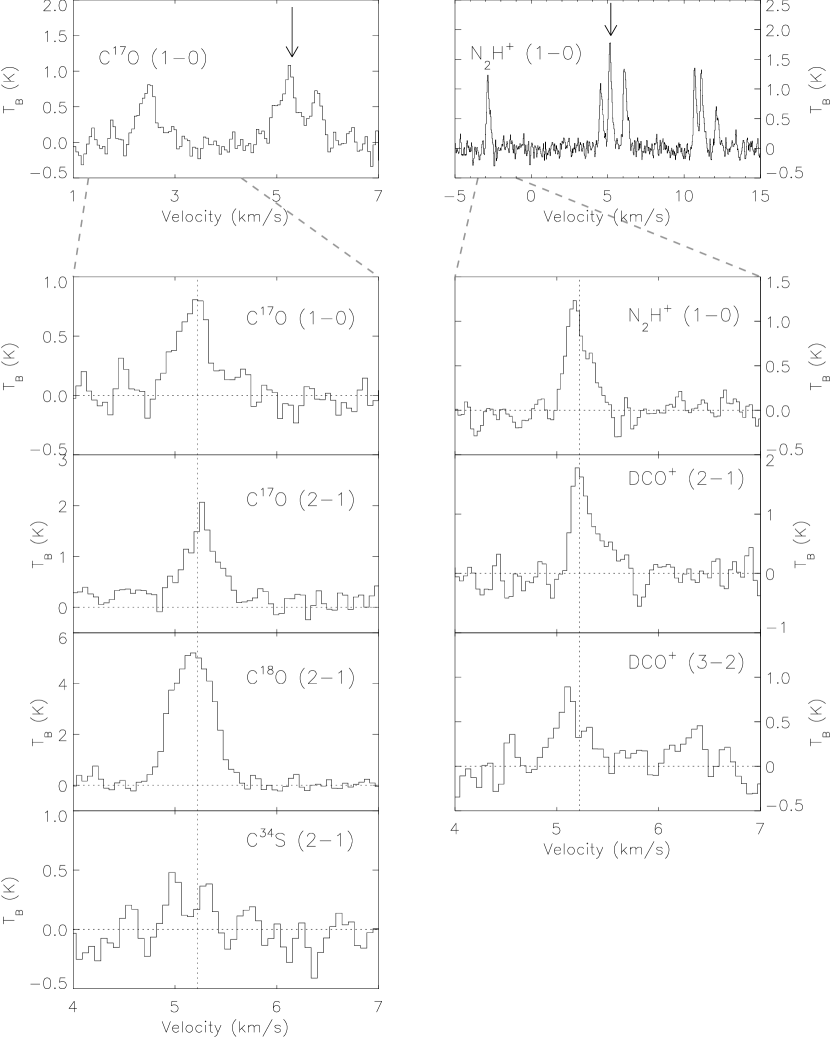
Figure 1.— The spectra taken at the (0,20) position, which is the peak of the dust emission map. The velocity scales on the spectra showing hyperfine structure are only correct for the marked component, whereas the enlarged portion of the spectra has been recentered at the frequency of the isolated component. The vertical dotted line shows the LSR velocity of the weakest component of the N₂H⁺(1-0) spectrum, as determined by a Gaussian fit, for comparison.

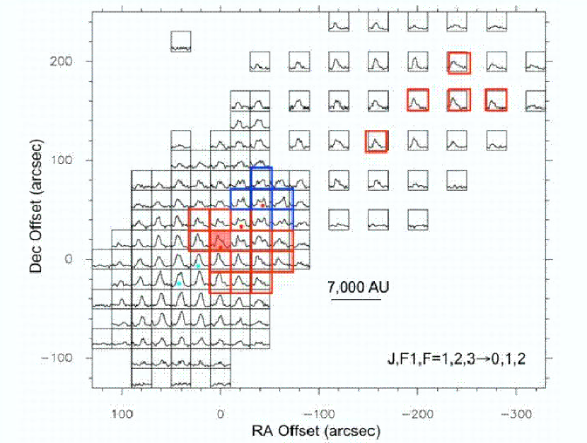
Figure 2.— Spectra of the F₁,F = 2,3 $\rightarrow$ 1,2 hyperfine component of ${\rm N}_{2}{\rm H}^{+}$ across the whole TMC–1C mapped region. Red boxes mark spectra consistent with inward motions, whereas blue boxes mark spectra with outflow signatures (see Sect. 4.3). Colored dots indicate those positions displayed in Fig. 9. The red-filled box mark the position of the continuum dust emission peak. The asymmetry in the high density tracer ${\rm N}_{2}{\rm H}^{+}$ is observed in an extended region, larger than that previously found in other evolved pre–stellar cores. See Fig. 4 for contours of column density based on dust emission.

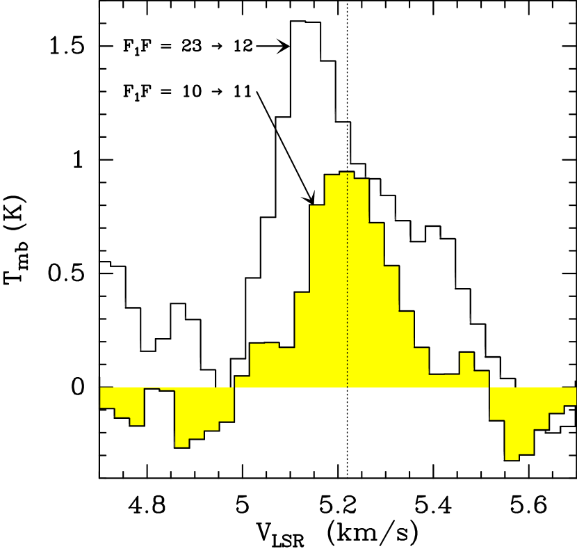
Figure 3.— Profile of the main F₁,F = 23 $\rightarrow$ 12 hyperfine component of ${\rm N}_{2}{\rm H}^{+}$(1–0) (white histogram) superposed on the spectrum of the weak F₁F = 10 $\rightarrow$ 11 component (yellow histogram) at the dust peak position. Note that the weak component is symmetric and peaks where the absorption of the main component is steepest, suggesting that this component is optically thin and can be used to estimate the column density and line width where the main group of hyperfines is affected by self-absorption.

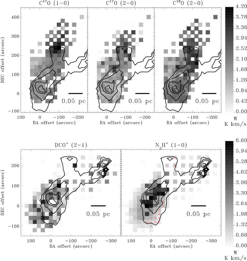
Figure 4.— Integrated intensity maps of (top left) C¹⁷O(1–0), (top middle) C¹⁷O(2–1), (top right) C¹⁸O(2–1), (bottom left) DCO⁺(2–1) and (bottom right) N₂H⁺(1–0). The C¹⁷O(1–0), C¹⁷O(2–1) and DCO⁺(2–1) integrated intensities have been scaled up by factors of 1.5, 2.0 and 5.0, respectively. For all spectra showing self-absorption, the N₂H⁺ integrated intensity has been calculated from the thinnest hyperfine component. The contours show the visual extinction derived from the dust emission, at levels of $A_{V}$ = 10, 25, 40, and 55 mag. The 1$\sigma$ uncertainties in the integrated intensity are $\sim$0.05, $\sim$0.06, $\sim$0.10, $\sim$0.07 and $\sim$0.08 K km s^-1 in C¹⁷O(1–0), C¹⁷O(2–1), C¹⁸O(2–1), DCO⁺(2–1) and N₂H⁺(1–0) respectively. The positions with large N₂H⁺ depletion and low column density have been marked with red crosses.

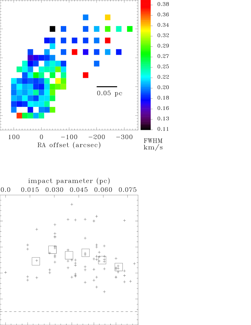
Figure 5.— (Top Panel) N₂H⁺(1-0) observed line width across the TMC–1C core. (Bottom Panel) N₂H⁺(1-0) observed line width (in km s^-1) vs. distance from the peak of the dust column density map. For those positions where the self–absorption is present, we used the width of the weak component as representative of the intrinsic line width of the (1-0) line. The crosses show the values at each position in the map with S/N $>$ 3, and the large squares are averages of the data with 15″ bins. The horizontal dashed line shows the thermal FWHM at 10 K for reference.

Figure 6.— The non-thermal line width plotted against the thermal line width for each transition observed, at the position of the dust emission peak. The thermal line width is calculated from an assumed gas temperature of 10 K. The error in the non-thermal line width is derived using the error in the FWHM of the Gaussian fit to the line. The line withs of C³⁴S(2–1) and ${\rm DCO}^{+}$(3–2) are highly uncertain, because of the strong absorption observed (see Fig. 2) and the plotted errors do not take the absorption into account. The NH₃ intrinsic line width is taken from Barranco & Goodman (1998). To make a fair comparison, all of the spectral line maps have been spatially smoothed to the $\sim$1′ resolution of the NH₃ map.

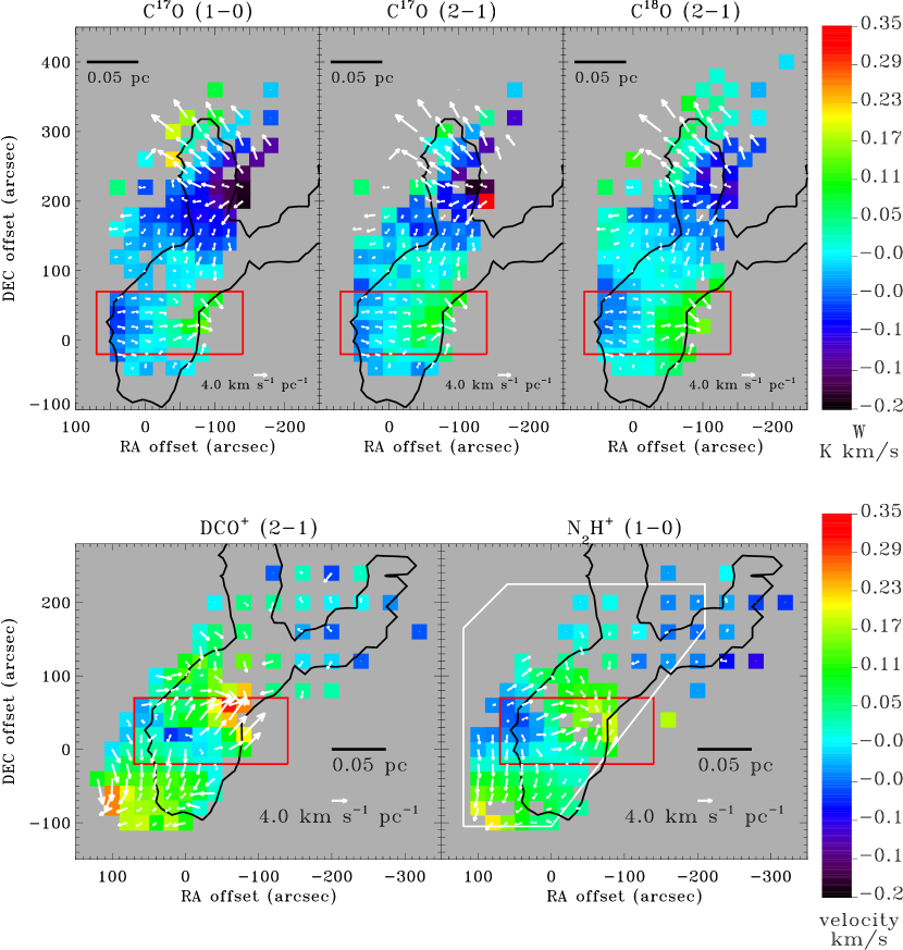
Figure 7.— Top Panels) The velocity field for C¹⁷O(1-0), C¹⁷O(2-1) and C¹⁸O(2-1). The black contour shows the A${}_{\rm V}=10$ mag boundary, and the arrows show the direction and magnitude of the line-of-sight velocity gradient, pointing from blue to red. The red box encloses a region with a velocity gradient similar to that of rotation as seen in the isotopologues of CO. In each map the velocity shown is the difference between the measured VLSR at each position and the velocity at the (0,0) position. The lengths of the arrows are proportional to the magnitude of the gradient, and is scaled to the labeled arrow. (Bottom Panels) velocity field for ${\rm DCO}^{+}$(2–1) and N₂H⁺(1–0) in TMC-1C. The red box encloses a region with a velocity gradient in isotopologues of CO that looks similar to that of rotation. The white box shows the region observed in NH₃ by Barranco & Goodman (1998).

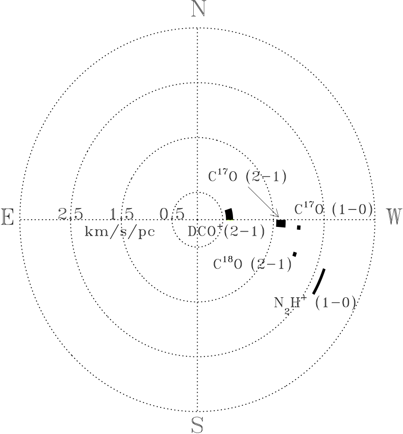
Figure 8.— The overall velocity gradient for each tracer in the region bounded by $-140<$ RA${}_{\rm offset}<70$ and $-20<$ DEC${}_{\rm offset}<70$, the region in the red box in Fig. 7 and 7. The dotted circles show the magnitude of gradients equal to 0.5, 1.5, 2.5 and 3.5 km s^-1 pc^-1.

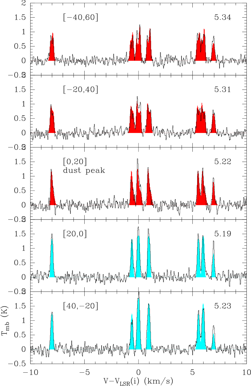
Figure 9.— ${\rm N}_{2}{\rm H}^{+}$(1–0) spectra (black histogram) along a South–East (bottom panel) to North–West (top panel) strip (see spectra labelled with colored dots in Fig. 2). Filled red histograms are two–layer model results, whereas light blue filled histograms are simply fits to the line, assuming one emitting layer and constant $T_{\rm ex}$ for the seven hyperfines. Offsets from Fig. 2 are in the top left of each panel. Numbers in the top right are the $V_{\rm LSR}$ velocities (in ${\rm km\,s}^{-1}$) from gaussian fits to the hfs structure. The parameters of the fits are in Table 3. Note that the redshifted absorption (and thus the infall velocity) is largest toward the dust peak and that the self-absorption is present towards the North–West but not towards the South–East.

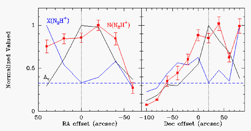
Figure 10.— Right ascension (left) and declination (right) cuts cross the TMC–1C core, passing through the dust peak position (black dotted line), of $A_{\rm V}$ (black curve), $N(\hbox{${\rm N}_{2}{\rm H}^{+}$})$ (red curve), and $X(\hbox{${\rm N}_{2}{\rm H}^{+}$})$ (blue curve) normalized to their maximum values (see text). The blue dashed line is the abundance value observed across L1544 (see Vastel et al. 2006). $X(\hbox{${\rm N}_{2}{\rm H}^{+}$})$ shows an anticorrelation with the dust profile, suggestive of some ${\rm N}_{2}{\rm H}^{+}$ depletion toward the dust center.

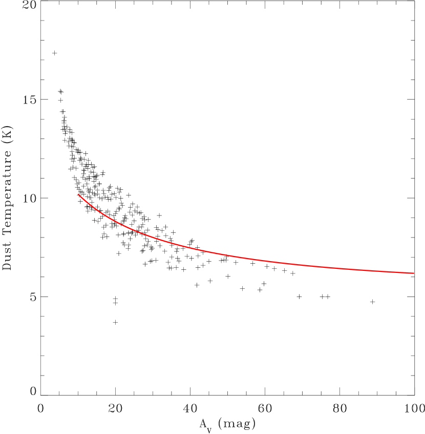
Figure 11.— The dust temperature plotted against the column density, derived from the dust emission maps at 450, 850 and 1200 µm. The spatial resolution of the data is 14″, resolving the innermost region of the core, with $A_{\rm V}$ $\simeq$ 90 mag and $T_{\rm dust}$ $\simeq$ 5 K. The solid red line shows the $T_{d}-A_{V}$ relation predicted for an externally heated pre-protostellar core by Zucconi et al. (2001, Eq. 26). Departures from spherical symmetry are probably causing the observed discrepancy between observations and (spherically symmetric) model predictions.

Figure 12.— (left) Excitation temperature of the ${\rm C}^{18}{\rm O}$(2–1) line. If this line is in LTE, the present data suggest a gas temperature decrease from about 12 K at the dust peak, to about 10 K at $\geq$ 1′ away from the dust peak (equivalent to a projected distance of $\geq$8,000 AU). But we believe that this is caused by the density drop traced by the ${\rm C}^{18}{\rm O}$(2–1) line (see text for details). (right) Brightness temperature ratio of the ${\rm C}^{17}{\rm O}$(1–0) and ${\rm C}^{17}{\rm O}$(2–1) lines as a function of distance from the dust (or $A_{\rm V}$) peak. The ratio increases with distance, suggesting that some physical property ($T_{\rm kin}$ and/or $n(\hbox{${\rm H}_{2}$})$) changes as well.

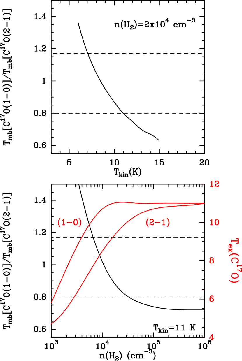
Figure 13.— Ratio of the ${\rm C}^{17}{\rm O}$(1–0) and ${\rm C}^{17}{\rm O}$(2–1) brightness temperatures as a function of (Top) gas temperature, for a fixed value of the volume density ($n({\rm\hbox{${\rm H}_{2}$}})$ = 2$\times$10⁴ $\hbox{{\rm cm}}^{-3}$), and (Bottom) volume density, for a fixed value of the gas temperature ($T_{\rm kin}$ = 11 K). In both panels, $N(\hbox{${\rm C}^{17}{\rm O}$})$ = 10¹⁵ $\hbox{{\rm cm}}^{-2}$ and $\Delta v$ = 0.4 ${\rm km\,s}^{-1}$. The dashed horizontal lines enclose the observed range of $T_{\rm mb}$ ratios (see Fig. 12, right panel). Note that observations are both consistent with a gas temperature decrease (and high constant density), as well as with a volume density decrease (and constant gas temperature) away from the dust peak. We believe that the latter is a more plausible solution than the former.

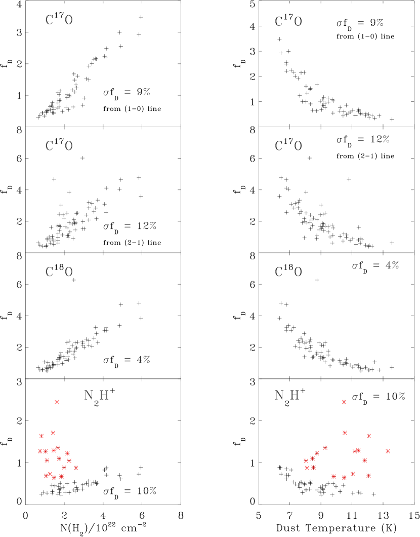
Figure 14.— (left) The depletion factor derived from molecular transitions observed with the IRAM 30m plotted against the column density derived from dust emission maps at 450, 850 and 1200 µm. The median percent error in the depletion (calculated from the RMS of the spectrum) is given in each panel. (right) Same as left, except that the depletion factor is plotted against the dust temperature. Those points with anomalously high ${\rm N}_{2}{\rm H}^{+}$depletion factors ($N_{H_{2}}<3\times 10^{22}$ and $f_{D}>0.6$) are shown in red, and their positions are shown with red crosses in Fig. 4. The ${\rm N}_{2}{\rm H}^{+}$ depletion factor goes below 1 because of our arbitrary choice of the ${\rm N}_{2}{\rm H}^{+}$ column density (see text).

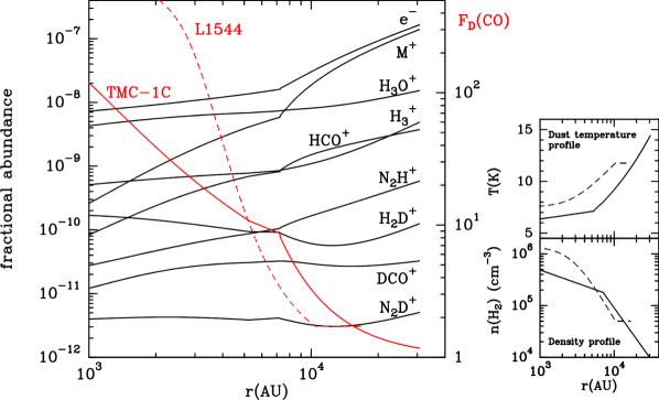
Figure 15.— (Left panel) Fractional abundances of important molecular ions as a function of radius, calculated by the best–fit model for TMC–1C (i.e. the one that best reproduces the observed column densities, see text). The red curves are depletion factors within TMC-1C ($F_{\rm D}(CO)$, see the scale in the right y-axis) and, for comparison, within L1544 (dashed red curve, from Vastel et al. 2006). The discontinuity in the fractional abundance profiles is due to the particular density profile used. (Right panel) Temperature and density profiles in TMC–1C, derived by Schnee et al. (2007) and used in the chemical model. Dashed curves refer to L1544 (adopted by Vastel et al. 2006).

References

- Aikawa et al. (2005) Aikawa, Y., Herbst, E., Roberts, H., & Caselli, P. 2005, ApJ, 620, 330
- Aikawa et al. (2001) Aikawa, Y., Ohashi, N., Inutsuka, S.-i., Herbst, E., & Takakuwa, S. 2001, ApJ, 552, 639
- Barranco & Goodman (1998) Barranco, J. A., & Goodman, A. A. 1998, ApJ, 504, 207
- Belloche & André (2004) Belloche, A., & André, P. 2004, A&A, 419, L35
- Benson et al. (1998) Benson, P. J., Caselli, P., & Myers, P. C. 1998, ApJ, 506, 743
- Bergin et al. (2006) Bergin, E. A., Maret, S., van der Tak, F. F. S., Alves, J., Carmody, S. M., & Lada, C. J. 2006, ApJ, 645, 369
- Bergin et al. (2002) Bergin, E. A., Alves, J., Huard, T., & Lada, C. J. 2002, ApJ, 570, L101
- Bergin & Langer (1997) Bergin, E. A., & Langer, W. D. 1997, ApJ, 486, 316
- Bianchi et al. (2000) Bianchi, S., Davies, J. I., Alton, P. B., Gerin, M., & Casoli, F. 2000, A&A, 353, L13
- Bisschop et al. (2006) Bisschop, S. E., Fraser, H. J., Öberg, K. I., van Dishoeck, E. F., & Schlemmer, S. 2006, A&A, 449, 1297
- Bonnell & Bate (2006) Bonnell, I. A., & Bate, M. R. 2006, MNRAS, 370, 488
- Bourke et al. (2006) Bourke, T. L., et al. 2006, ApJ, 649, L37
- Caselli et al. (1999) Caselli, P., Walmsley, C. M., Tafalla, M., Dore, L., & Myers, P. C. 1999, ApJ, 523, L165
- Caselli et al. (2002a) Caselli, P., Walmsley, C. M., Zucconi, A., Tafalla, M., Dore, L., & Myers, P. C. 2002, ApJ, 565, 331
- Caselli et al. (2002b) Caselli, P., Walmsley, C. M., Zucconi, A., Tafalla, M., Dore, L., & Myers, P. C. 2002, ApJ, 565, 344 5A
- Ceccarelli et al. (2006) Ceccarelli, C., Caselli, P., Herbst, E., Tielens, X., & Caux, E. 2006, in Protostars & Planets V, in press (astro-ph/0603018)
- Ciolek & Basu (2000) Ciolek, G. E., & Basu, S. 2000, ApJ, 529, 925
- Colling et al. (2003) Collings, M. P., Dever, J. W., Fraser, H. J., McCoustra, M. R. S., & Williams, D. A. 2003, ApJ, 583, 1058
- Crapsi et al. (2007) Crapsi, A., Caselli, P., Walmsley, C. M., Tafalla, M. 2005, A&A, in press (astro-ph/0705.0471)
- Crapsi et al. (2005) Crapsi, A., Caselli, P., Walmsley, C. M., Myers, P. C., Tafalla, M., Lee, C. W., & Bourke, T. L. 2005, ApJ, 619, 379
- Crapsi et al. (2004) Crapsi, A., Caselli, P., Walmsley, C. M., Tafalla, M., Lee, C. W., Bourke, T. L., & Myers, P. C. 2004, A&A, 420, 957
- Dalgarno & Lepp (1984) Dalgarno, A., & Lepp, S. 1984, ApJ, 287, L47
- Daniel et al. (2006) Daniel, F., Cernicharo, J., & Dubernet, M.-L. 2006, ApJ, 648, 461
- De Vries & Myers (2005) De Vries, C. H., & Myers, P. C. 2005, ApJ, 620, 800
- Di Francesco et al. (2006) Di Francesco, J., Evans, N. J., II, Caselli, P., Myers, P. C., Shirley, Y., Aikawa, A., & Tafalla, M. 2006, in Protostars & Planets V, astro-ph/0602379
- Dore et al. (2004) Dore, L., Caselli, P., Beninati, S., Bourke, T., Myers, P. C., & Cazzoli, G. 2004, A&A, 413, 1177
- Ehrenfreund & Charnley (2000) Ehrenfreund, P., & Charnley, S. B. 2000, ARA&A, 38, 427
- Evans et al. (2001) Evans, N. J., II, Rawlings, J. M. C., Shirley, Y. L., & Mundy, L. G. 2001, ApJ, 557, 193
- Frerking et al. (1982) Frerking, M. A., Langer, W. D., & Wilson, R. W. 1982, ApJ, 262, 590
- Galli et al. (2002) Galli, D., Walmsley, M., & Gonçalves, J. 2002, A&A, 394, 275
- Goldsmith et al. (1997) Goldsmith, P. F., Bergin, E. A., & Lis, D. C. 1997, ApJ, 491, 615
- Goodman et al. (1998) Goodman, A. A., Barranco, J. A., Wilner, D. J., & Heyer, M. H. 1998, ApJ, 504, 223
- Goodman et al. (1993) Goodman, A. A., Benson, P. J., Fuller, G. A., & Myers, P. C. 1993, ApJ, 406, 528
- Gottlieb et al. (2003) Gottlieb, C. A., Myers, P. C., & Thaddeus, P. 2003, ApJ, 588, 655
- Hasegawa & Herbst (1993) Hasegawa, T. I., & Herbst, E. 1993, MNRAS, 263, 589
- Hirota et al. (2002) Hirota, T., Ito, T., & Yamamoto, S. 2002, ApJ, 565, 359
- Holland et al. (1999) Holland, W. S., et al. 1999, MNRAS, 303, 659
- Kenyon et al. (1994) Kenyon, S. J., Dobrzycka, D., & Hartmann, L. 1994, AJ, 108, 1872
- Klessen et al. (2005) Klessen, R. S., Ballesteros-Paredes, J., Vázquez-Semadeni, E., & Durán-Rojas, C. 2005, ApJ, 620, 786
- Kramer et al. (1999) Kramer, C., Alves, J., Lada, C. J., Lada, E. A., Sievers, A., Ungerechts, H., & Walmsley, C. M. 1999, A&A, 342, 257
- Kreysa et al. (1999) Kreysa, E., Gemünd, H.-P., Gromke, J. 1999 Infrared Phys. Techn. 40, 191
- Lada et al. (2003) Lada, C. J., Bergin, E. A., Alves, J. F., & Huard, T. L. 2003, ApJ, 586, 286
- Lee et al. (2004) Lee, C. W., Myers, P. C., & Plume, R. 2004, ApJS, 153, 523
- Lee et al. (2003) Lee, J.-E., Evans, N. J., II, Shirley, Y. L., & Tatematsu, K. 2003, ApJ, 583, 789
- Lee et al. (1996) Lee, H.-H., Bettens, R. P. A., & Herbst, E. 1996, A&AS, 119, 111
- Mathis et al. (1977) Mathis, J. S., Rumpl, W., & Nordsieck, K. H. 1977, ApJ, 217, 425
- McKee (1989) McKee, C. F. 1989, ApJ, 345, 782
- Meyer et al. (1998) Meyer, D. M., Jura, M., & Cardelli, J. A. 1998, ApJ, 493, 222
- Meyer et al. (1997) Meyer, D. M., Cardelli, J. A., & Sofia, U. J. 1997, ApJ, 490, L103
- Myers (2005) Myers, P. C. 2005, ApJ, 623, 280
- Myers et al. (1996) Myers, P. C., Mardones, D., Tafalla, M., Williams, J. P., & Wilner, D. J. 1996, ApJ, 465, L133
- Öberg et al. (2005) Öberg, K. I., van Broekhuizen, F., Fraser, H. J., Bisschop, S. E., van Dishoeck, E. F., & Schlemmer, S. 2005, ApJ, 621, L33
- Ossenkopf & Henning (1994) Ossenkopf, V., & Henning, T. 1994, A&A, 291, 943
- Pagani et al. (2005) Pagani, L., Pardo, J.-R., Apponi, A. J., Bacmann, A., & Cabrit, S. 2005, A&A, 429, 181
- Penzias (1981) Penzias, A. A. 1981, ApJ, 249, 518
- Pierce-Price et al. (2000) Pierce-Price, D., et al. 2000, ApJ, 545, L121
- Redman et al. (2002) Redman, M. P. Rawlings, J. M. C., Nutter, D. J., Ward-Thompson, D., & Williams, D. A. 2002, MNRAS, 337, L17
- Roberts et al. (2004) Roberts, H., Herbst, E., & Millar, T. J. 2004, A&A, 424, 905
- Schnee & Goodman (2005) Schnee, S., & Goodman, A. 2005, ApJ, 624, 254
- Schnee et al. (2007) Schnee, S., Kauffman, J., Goodman, A. & Bertoldi, F. 2007, ApJ, in press.
- Schöier et al. (2005) Schöier, F. L., van der Tak, F. F. S., van Dishoeck, E. F., & Black, J. H. 2005, A&A, 432, 369
- Shematovich et al. (2003) Shematovich, V. I., Wiebe, D. S., Shustov, B. M., & Li, Z.-Y. 2003, ApJ, 588, 894
- Tafalla et al. (2004) Tafalla, M., Myers, P. C., Caselli, P., & Walmsley, C. M. 2004, Ap&SS, 292, 347
- Tafalla & Santiago (2004b) Tafalla, M., & Santiago, J. 2004, A&A, 414, L53
- Tafalla et al. (2002) Tafalla, M., Myers, P. C., Caselli, P., Walmsley, C. M., & Comito, C. 2002, ApJ, 569, 815
- Tafalla et al. (1998) Tafalla, M., Mardones, D., Myers, P. C., Caselli, P., Bachiller, R., & Benson, P. J. 1998, ApJ, 504, 900
- Taylor et al. (1998) Taylor, S. D., Morata, O., & Williams, D. A. 1998, A&A, 336, 309
- Umebayashi & Nakano (1990) Umebayashi, T., & Nakano, T. 1990, MNRAS, 243, 103
- van der Tak et al. (2007) van der Tak, F. F. S., Black, J. H., Schöier, F. L., Jansen, D. J., & van Dishoeck, E. F. 2007, A&A, 468, 627
- Vastel et al. (2006) Vastel, C., Caselli, P., Ceccarelli, C., Phillips, T., Wiedner, M. C., Peng, R., Houde, M., & Dominik, C. 2006, ApJ, 645, 1198
- Williams et al. (2006) Williams, J. P., Lee, C. W., & Myers, P. C. 2006, ApJ, 636, 952
- Williams et al. (1999) Williams, J. P., Myers, P. C., Wilner, D. J., & di Francesco, J. 1999, ApJ, 513, L61
- Wilson & Rood (1994) Wilson, T. L., & Rood, R. 1994, ARA&A, 32, 191
- Zucconi et al. (2001) Zucconi, A., Walmsley, C. M., & Galli, D. 2001, A&A, 376, 650