Level crossing in the three-body problem for strongly interacting fermions
in a harmonic trap

Abstract

We present a solution of the three-fermion problem in a harmonic potential across a Feshbach resonance. We compare the spectrum with that of the two-body problem and show that it is energetically unfavorable for the three fermions to occupy one lattice site rather than two. We also demonstrate the existence of an energy level crossing in the ground state with a symmetry change of its wave function, suggesting the possibility of a phase transition for the corresponding many-body case.

I Introduction

Ultracold atoms, tuned with Feshbach resonance, offer a great opportunity to study strongly correlated many-body physics in a controlled fashion. For such strongly interacting systems, in general there is no well-controlled approximation method to solve the many-body physics. Exact solution of few-body problems plays an important role in understanding the corresponding many-body systems. Few-body (three- or four-body) problems have been solved for strongly interacting bosons or fermions in free space Petrov03 , in a quasi-one-dimensional configuration Mora05 , and in a three-dimensional (3D) harmonic trap for bosons Stoll05 or fermions in the unitary limit Werner06 ; Chang07 .

In this paper, we add to this sort of examples by exactly solving the three-body problem for strongly interacting two-component fermions in a 3D harmonic trap across resonance. This work has two main motivations: Firstly, the situation considered here is relevant for experiments where one loads strongly interacting two component fermions into a deep 3D optical lattice lat . For each site that can be approximated with a harmonic potential, one could have two identical fermions (spin-$\uparrow$) strongly interacting with another distinct fermion (spin-$\downarrow$). The three-body problem for equal mass fermions turns out to be very different from the corresponding case for bosons. Instead of a hierarchy of bound Efimov states for bosons Stoll05 , we show that there is always a significant energy penalty for three fermions to occupy the same lattice site ($\uparrow\uparrow\downarrow$) instead of two ($\uparrow\downarrow+\uparrow$). This result justifies an important assumption made in the derivation of an effective many-body Hamiltonian for this system Duan05 . Secondly, we analyze the ground-state structure of the three-body problem and show that as one scans the 3D scattering length, there is a level crossing between the lowest-lying three-fermion energy eigenstates, which have s- or p-wave symmetries respectively in the limit as two atoms are contracted to form a dimer. This level crossing with a symmetry change may correspond a quantum phase transition in the many-body case where one has spin-polarized fermi gas loaded into an optical lattice. The latter system with polarized fermions has raised strong interest recently in both theory and experiments exp06 ; theory06 .

II Methods

The method here is based on manipulation of a Lippmann-Schwinger equation for the wavefunction, with the formalism similar to the one presented in Ref. Mora05 . As is standard, we separate the center-of-mass degree of freedom via an orthogonal transformation of variables, leaving the trapping potential diagonal in the new coordinates. The Schrödinger equation for the relative degrees of freedom is then

$$\left[-\frac{\hbar^{2}}{m_{0}}\left(\nabla_{\mathbf{x}}^{2}+\nabla_{\mathbf{y}}^{2}\right)+\frac{1}{4}m_{0}\omega^{2}\left(\mathbf{x}^{2}+\mathbf{y}^{2}\right)-E\right]\Psi\left(\mathbf{x},\mathbf{y}\right)\\ =-\sum_{\pm}V\left(\mathbf{r}_{\pm}\right)\Psi\left(\mathbf{x},\mathbf{y}\right)\,,$$ (1)

where $m_{0}$ is the atomic mass, $\omega$ is the trap frequency, $\mathbf{y}$ is the vector between the two $\uparrow$ fermions, $\sqrt{3}\mathbf{x}/2$ is a vector from the center of mass of the two $\uparrow$ fermions to the $\downarrow$ fermion, and $\mathbf{r}_{\pm}=\sqrt{3}\mathbf{x}/2\pm\mathbf{y}/2$ are the vectors from the $\downarrow$ fermion to each of the two $\uparrow$ fermions. We approximate the short-range interaction between fermions with the usual zero-range pseudopotential Huang56 $V\left(\mathbf{r}\right)=\frac{4\pi\hbar^{2}a}{m_{0}}\delta\left(\mathbf{r}\right)\frac{\partial}{\partial r}\left(r\cdot\right)$, where $a$ is the 3D s-wave scattering length tunable through the Feshbach resonance.

The above contact interaction is equivalent to imposing boundary conditions $\Psi\left(\mathbf{x},\mathbf{y}\right)\simeq\mp\frac{f\left(\mathbf{r}_{\perp,\pm}\right)}{4\pi\mathbf{r}_{\pm}}\left(1-\frac{\mathbf{r}_{\pm}}{a}\right)$ for $\mathbf{r}_{\pm}\rightarrow 0$, where the $\mathbf{r}_{\perp,\pm}=\mathbf{x}/2\mp\sqrt{3}\mathbf{y}/2$ are proportional to the distances between the center of mass of an $\uparrow\downarrow$ pair and an $\uparrow$ fermion. The overall $\mp$ sign ensures the antisymmetry of the wavefunction upon swapping the identical fermions. The undetermined function $f\left(\mathbf{r}_{\perp,\pm}\right)$, after a rescaling of the argument, is the relative atom-dimer wavefunction that results when two of the fermions form a tightly bound pair. Solving for this asymptotic wavefunction $f\left(\mathbf{r}_{\perp,\pm}\right)$ fully determines $\Psi\left(\mathbf{x},\mathbf{y}\right)$.

Since $V\left(\mathbf{r}_{\pm}\right)$ only acts at $\mathbf{r}_{\pm}=0$, we use the asymptotic form of $\Psi$ when computing $V\left(\mathbf{r}_{\pm}\right)\Psi$. The formal solution can then be written as

$$\Psi\left(\mathbf{x},\mathbf{y}\right)=\int d\mathbf{x^{\prime}}d\mathbf{y^{\prime}}G_{E}^{\left(2\right)}\left(\mathbf{x},\mathbf{y};\mathbf{x^{\prime}},\mathbf{y^{\prime}}\right)\\ \times\sum_{\pm}\frac{\mp\hbar^{2}f\left(\mathbf{r^{\prime}}_{\perp,\pm}\right)}{m_{0}}\delta\left(\mathbf{r^{\prime}}_{\pm}\right)$$ (2)

where the two-particle Green’s function is given by

$$G_{E}^{\left(2\right)}\left(\mathbf{x},\mathbf{y};\mathbf{x^{\prime}},\mathbf{y^{\prime}}\right)=\sum_{\lambda_{1}\lambda_{2}}\frac{\psi_{\lambda_{1}}\left(\mathbf{x}\right)\psi_{\lambda_{2}}\left(\mathbf{y}\right)\psi_{\lambda_{1}}^{\ast}\left(\mathbf{x^{\prime}}\right)\psi_{\lambda_{2}}^{\ast}\left(\mathbf{y^{\prime}}\right)}{E_{\lambda_{1}}+E_{\lambda_{2}}-E}$$ (3)

The $\psi_{\lambda_{i}}\left(\mathbf{x}\right)$ are the single-particle eigenfunctions with eigenenergies $E_{\lambda_{i}}$ for the reduced mass $m_{0}/2$. Here we use spherical coordinates for the three-dimensional harmonic trap, so the quantum numbers are $\lambda=\left(n,l,m\right)$, $n=0,1,2,...$; $l=0,1,2,...$; $m=-l,-l+1,...,l-1,l$. The eigenenergies are $E_{\lambda}=\left(2n+l+3/2\right)\hbar\omega$ and the eigenfunctions are $\psi_{\lambda}\left(\mathbf{r}\right)=R_{nl}\left(r\right)Y_{l}^{m}\left(\theta,\phi\right)$, where the $Y_{l}^{m}\left(\theta,\phi\right)$ are the standard spherical harmonics. The radial wavefunction is given by Powell61

$$R_{nl}\left(r\right)=\sqrt{\frac{2n!/d^{3}}{\left(n+l+1/2\right)!}}e^{-r^{2}/2d^{2}}\left(\frac{r}{d}\right)^{l}L_{n}^{l+1/2}\left(r^{2}/d^{2}\right)$$ (4)

where $d=\sqrt{\frac{2\hbar}{m_{0}\omega}}$ is the length scale of the trap and the $L_{n}^{k}\left(r\right)$ are associated Laguerre polynomials.

We can make use of the invariance of $G_{E}^{\left(2\right)}$ and the integration measure under an orthogonal transformation of variables to rewrite Eq. (2) in terms of $\mathbf{r}\equiv\mathbf{r}_{-}$ and $\mathbf{r}_{\perp}\equiv\mathbf{r}_{\perp,-}$,

$$\Psi\left(\mathbf{r},\mathbf{r}_{\perp}\right)=\frac{\hbar^{2}}{m_{0}}\int d\mathbf{r}_{\perp}^{\prime}f\left(\mathbf{r}_{\perp}^{\prime}\right)\biggl{[}G_{E}^{\left(2\right)}\left(\mathbf{r},\mathbf{r}_{\perp};0,\mathbf{r}_{\perp}^{\prime}\right)\\ -G_{E}^{\left(2\right)}\left(\frac{\mathbf{r}}{2}+\frac{\sqrt{3}\mathbf{r}_{\perp}}{2},\frac{\sqrt{3}\mathbf{r}}{2}-\frac{\mathbf{r}_{\perp}}{2};0,\mathbf{r}_{\perp}^{\prime}\right)\biggr{]}$$ (5)

We can also decompose the asymptotic atom-dimer wavefunction in terms of the complete set of single-particle wavefunctions, $f\left(\mathbf{r}_{\perp}\right)=\sum_{\lambda}f_{\lambda}\psi_{\lambda}\left(\mathbf{r}_{\perp}\right)$. Then Eq. (5) becomes

$$\Psi\left(\mathbf{r},\mathbf{r}_{\perp}\right)=d^{2}\hbar\omega\sum_{\lambda}\biggl{[}G_{E-E_{\lambda}}\left(\mathbf{r},0\right)\psi_{\lambda}\left(\mathbf{r}_{\perp}\right)\\ -G_{E-E_{\lambda}}\left(\frac{\mathbf{r}}{2}+\frac{\sqrt{3}\mathbf{r}_{\perp}}{2},0\right)\psi_{\lambda}\left(\frac{\sqrt{3}\mathbf{r}}{2}-\frac{\mathbf{r}_{\perp}}{2}\right)\biggr{]}f_{\lambda}$$ (6)

where $G_{E}$ is the single-particle Green’s function,

$$G_{E}\left(\mathbf{r},0\right)=\sum_{\lambda}\frac{\psi_{\lambda}\left(\mathbf{r}\right)\psi_{\lambda}^{\ast}\left(0\right)}{E_{\lambda}-E}\\ =\frac{e^{-r^{2}/2d^{2}}}{2\pi^{3/2}d^{3}\hbar\omega}\Gamma\left(\frac{\frac{3}{2}-E/\hbar\omega}{2}\right)U\left(\frac{\frac{3}{2}-E/\hbar\omega}{2},\frac{3}{2},\frac{r^{2}}{d^{2}}\right)$$ (7)

Busch98 , and $U$ is the confluent hypergeometric function. Note that the three-fermion wavefunction is fully determined by $f\left(\mathbf{r}_{\perp}\right)$ and that if we consider Eq. (6) in the limit as $\mathbf{r}\rightarrow 0$, we obtain a self-consistent equation for $f\left(\mathbf{r}_{\perp}\right)$ by using the boundary conditions. After some work, we obtain

$$\sum_{\lambda^{\prime}}A_{\lambda\lambda^{\prime}}f_{\lambda^{\prime}}=\left[\frac{d}{a}-2\frac{\Gamma\left(\frac{3/2+E_{\lambda}/\hbar\omega-E/\hbar\omega}{2}\right)}{\Gamma\left(\frac{1/2+E_{\lambda}/\hbar\omega-E/\hbar\omega}{2}\right)}\right]f_{\lambda}$$ (8)

where

$$A_{\lambda\lambda^{\prime}}=\int\!\!\!\!\frac{d\mathbf{r}_{\perp}}{4\pi d^{3}\hbar\omega}G_{E-E_{\lambda^{\prime}}}\!\left(\!\frac{\sqrt{3}\mathbf{r}_{\perp}}{2},0\!\right)\psi_{\lambda}^{\ast}\left(\mathbf{r}_{\perp}\right)\psi_{\lambda^{\prime}}\!\left(\frac{\mathbf{-r}_{\perp}}{2}\right)$$ (9)

III Results

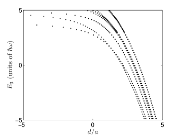
Figure 1: Energy vs. inverse scattering length.

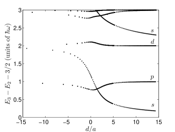
Figure 2: Difference between three-fermion energy and two-fermion energy plus one-fermion energy vs. inverse scattering length.

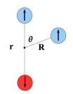
Figure 3: (Color online) Relative coordinates for the three-fermion problem. In terms of variables used in Eq. (6), $r=\left|\mathbf{r}\right|$, $R=\sqrt{3}\left|\mathbf{r}_{\perp}\right|/2$.

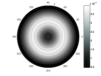
(a) $n=0$, $l=0$, $m=0$

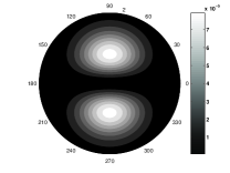
(b) $n=0$, $l=1$, $m=\pm 1$

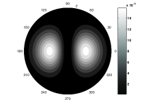
(c) $n=0$, $l=1$, $m=0$

Figure 4: Contour plots of $r^{2}\left|\Psi\left(r,R,\theta\right)\right|^{2}_{r\rightarrow 0}$ as a function of $R$ and $\theta$ for $r/d\simeq 0$ and $d/a\simeq 0$.

(a) $n=0$, $l=0$, $m=0$

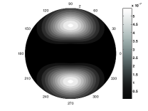
(b) $n=0$, $l=1$, $m=\pm 1$

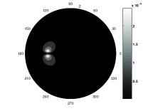
(c) $n=0$, $l=1$, $m=0$

Figure 5: Contour plots of $r^{2}R^{2}\left|\sin\theta\Psi\left(r,R,\theta\right)\right|^{2}$ as a function of $R$ and $\theta$ for $r/d=2$ and $d/a\simeq 0$.

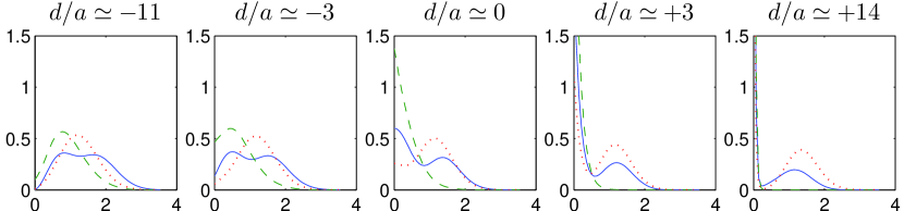
(a) Normalized probability density vs. $r/d$

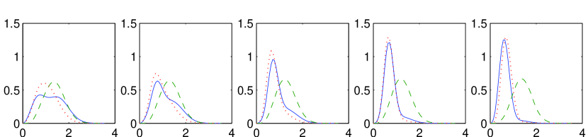
(b) Normalized probability density vs. $R/d$

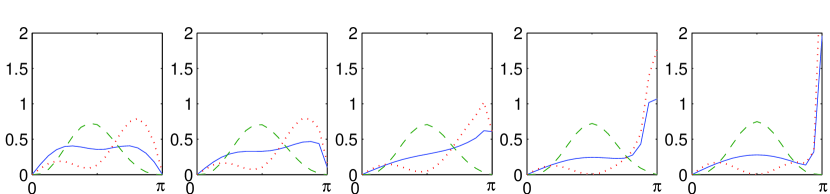
(c) Normalized probability density vs. $\theta$

Figure 6: (Color online) Normalized probability density distribution functions of variables defined in Fig. 3 for various scattering lengths. The solid line is for the $n=0$, $l=0$, $m=0$ state; the dashed line is for the $n=0$, $l=1$, $m=\pm 1$ state; and the dotted line is for the $n=0$, $l=1$, $m=0$ state.

We anticipate that the low-energy physics should be contained in a truncated Hilbert space containing only the lowest few asymptotic atom-dimer energy levels. Then Eq. (8) is easily solved numerically. We have checked that, indeed, the solution for the ground state and the first excited manifold become insensitive to the cutoff, as long as the first four or five atom-dimer energy levels are included. For all results presented in this paper, we have kept the first five energy levels. Because of the degeneracy of the excited levels, Eq. (8) becomes a $35\times 35$ matrix equation. For a given energy, we solve numerically to obtain the corresponding scattering length and eigenstate. By sweeping through a range of energies, we map out the spectrum shown in Fig. 1. At unitarity, our result for the low-energy spectrum agrees with the analytic result of Ref. Werner06 . Upon careful inspection, one can discern the presence of level crossings. More usefully, in Fig. 2 we display the difference between the energy of three fermions in a single lattice site and the energy of two fermions ($\uparrow\downarrow$) in the site and the extra fermion alone in a separate site. Here we have used the well-known exact solution for the two-body energy $E_{2}$ Busch98 ,

$$\frac{d}{a}=2\frac{\Gamma\left(\frac{3/2-E_{2}/\hbar\omega}{2}\right)}{\Gamma\left(\frac{1/2-E_{2}/\hbar\omega}{2}\right)}$$ (10)

Figure 2 is our main result. There are two main features we would like to point out. First, it is clear that it is energetically favorable for atoms in a lattice to arrange themselves such that there are less than three atoms per site, regardless of the scattering length. This has already been assumed in the derivation of an effective many-body Hamiltonian for atoms in an optical lattice across a Feshbach resonance Duan05 , and is confirmed by Fig. 2. Second, the level crossing in the ground state is now quite evident. On the positive scattering length side of the crossing (the BEC side, where the many-body system forms a Bose-Einstein condensate of bound dimers), the ground state is nondegenerate. On the other side (the BCS side, where the many-body system forms a Bardeen-Cooper-Schrieffer superfluid of atomic Cooper pairs), it is triply degenerate. Other crossings appear in the excited spectrum, although to obtain quantitatively accurate results for these one should include higher modes when solving Eq. (8).

The origin of the level crossing is the differing symmetries of the eigenstates. For very small, positive scattering length (deep BEC side), formation of tightly bound dimers is favorable, so the state should behave as the ground state of the relative atom-dimer motion, which has s-wave symmetry. For very small, negative scattering length (deep BCS side), the atoms are essentially non-interacting, so the ground state comprises two atoms ($\uparrow\downarrow$) in the ground state of the trap plus the third in the first excited state of the trap (which is triply degenerate) because of Pauli exclusion. So, on the deep BCS side, the ground state has p-wave symmetry. Due to the rotational symmetry of a spherical harmonic trap, the total angular momentum of the three particles should be a conserved quantity. However, from the above analysis, this quantity has different values for the ground state in the deep BEC and deep BCS limits. Therefore, there must be a ground-state level crossing for this system as one scans the scattering length. If one considers multiple lattice sites with each site having on average two spin $\uparrow$ and one spin $\downarrow$ atoms (which could be realized with polarized fermions in an optical lattice with appropriate filling number and population imbalance), as the three-body problem has a level crossing with different ground state degeneracies in the BCS and the BEC limits, there could be a corresponding quantum phase transition for this many-body system (with small tunneling between lattice sites) as one scans the scattering length.

The wavefunction given in Eq, (6) does not generally have definite relative angular momentum for any two fermions. However, in the limit as the distance between two distinguishable fermions goes to zero, the wavefunction takes on the symmetry of the asymptotic atom-dimer wavefunction in the remaining coordinates. This is a relative angular momentum eigenstate due to the spherical symmetry of the limiting case. With the relative coordinates defined by Fig. 3, the symmetry of the wavefunction as a function of $R$ and $\theta$ in the limit as $r$ goes to zero is shown by Fig. 4. For finite $r$, the $m=0$ wavefunctions are affected by the asymmetry and take nontrivial shapes. We have plotted an example in Fig. 5. Note that in this figure we include a factor of $\sin\theta$ since the wavefunction itself diverges at $R=r/2$, $\theta=\pi$ according to the boundary conditions we have imposed. On the BEC side, the lobes are tightly bunched near $\theta=\pi$, but on the BCS side they spread around as expected.

In general, the eigenstates are rather difficult to visualize, since they depend nontrivially on three spatial variables as well as the scattering length. However, one can get some idea of the evolution of the eigenstates from Fig. 6, which shows the normalized probability density as a function of the variables introduced in Fig. 3 for various scattering lengths. In each subplot we have numerically integrated over the other two variables to obtain a one-dimensional function. The dimer size, $r$, clearly decreases in size as one enters the BEC regime, developing a strong peak at the origin. However, as is clear from Fig. 3, there are two ways to form a tightly bound dimer (due to the two identical spin $\uparrow$ atoms) and we have arbitrarily chosen one to define the origin $r=0$. So it is not surprising that we see a more diffuse second peak at large distance $r$, corresponding to the dimer forming between the spin $\downarrow$ and the other spin $\uparrow$ atom. This is also the meaning of the spike at $\theta=\pi$ on the BEC side.

IV Summary

We have found the low-lying energy levels of three fermions in a harmonic trap and examined the corresponding wavefunctions. The ground state has s-wave symmetry on the BEC side of Feshbach resonance and has p-wave symmetry on the BCS side. In the resonance region there is a level crossing, which may indicate a phase transition in the corresponding many-body case. We also note that, in the vicinity of resonance, the energy of three atoms in a single site is greater than their energy if they are in two sites, with a gap on the order of the trap spacing, validating the approximation in Ref Duan05 .

This work was supported by the MURI, the DARPA, the NSF award (0431476), the DTO under ARO contracts, and the A. P. Sloan Fellowship.

Note added: After completion of this work, we became aware of a recent work Stetcu07 which treats the trapped three-fermion problem with a different approximation method.

References

- (1) D.S. Petrov, Phys. Rev. A 67, 010703(R) (2003); D.S. Petrov, C. Salomon, G.V. Shlyapnikov, Phys. Rev. Lett. 93, 090404 (2004); E. Braaten, H.-W. Hammer, Phys.Rept. 428, 259-390 (2006).
- (2) C. Mora, R. Egger, A.O. Gogolin, and A. Komnik, Phys. Rev. Lett. 93, 170403 (2004); C. Mora, A. Komnik, R. Egger, and A. O. Gogolin, Phys. Rev. Lett. 95, 080403 (2005).
- (3) S. Jonsell, H. Heiselberg and C.J. Pethick, Phys. Rev. Lett. 89, 250401 (2002); M. Stoll and T. Köhler, Phys. Rev. A 72, 022714 (2005).
- (4) F. Werner and Y. Castin, Phys. Rev. Lett. 97, 150401 (2006).
- (5) S. Y. Chang and G. F. Bertsch, Phys. Rev. A 76, 021603(R) (2007).
- (6) T. Stöferle, H. Moritz, K. Günter, M. Köhl, T. Esslinger Phys. Rev. Lett. 96, 030401 (2006); J.K. Chin et al., Nature London 443, 961 (2006).
- (7) L.-M. Duan, Phys. Rev. Lett. 95, 243202 (2005); arXiv:0706.2161.
- (8) M.W. Zwierlein, A. Schirotzek, C.H. Schunck, and W. Ketterle, Science 311, 492 (2006); G.B. Partridge, W. Li, R.I. Kamar, Y. Liao, and R.G. Hulet, Science 311, 503 (2006).
- (9) D. E. Sheehy, L. Radzihovsky, cond-mat/0607803; W. Yi, L.-M. Duan, Phys. Rev. A 73, 031604(R) (2006); T. N. De Silva, E. J. Mueller, Phys. Rev. Lett. 97, 070402 (2006).
- (10) Kerson Huang and C.N. Yang, Phys. Rev. 105, 767 (1957).
- (11) J.L. Powell and B. Crasemann, Quantum Mechanics (Addison-Wesley, Reading, MA, 1961), Chapter 7.
- (12) T. Busch, B.-G. Englert, K. Rzazewski, M. Wilkens, Found. Physics 28, 549 (1998).
- (13) I. Stetcu, B. R. Barrett, U. van Kolck, J. P. Vary, arXiv:0705.4335.