Short Gamma-Ray Bursts and Binary Mergers in Spiral and Elliptical Galaxies: Redshift Distribution and Hosts

Abstract

To critically assess the binary compact object merger model for short gamma ray bursts (GRBs) – specifically, to test whether the short GRB rates, redshift distribution and host galaxies are consistent with current theoretical predictions – it is necessary to examine models that account for the high-redshift, heterogeneous universe (accounting for both spirals and ellipticals). We present an investigation of predictions produced from a very large database of first-principle population synthesis calculations for binary compact mergers with neutron stars (NS) and black holes (BH), that sample a seven-dimensional space for binaries and their evolution. We further link these predictions to (i) the star formation history of the universe, (ii) a heterogeneous population of star-forming galaxies, including spirals and ellipticals, and (iii) a simple selection model for bursts based on flux-limited detection. We impose a number of constraints on the model predictions at different quantitative levels: short GRB rates and redshift measurements, and, for NS-NS, the current empirical estimates of Galactic merger rates derived from the observed sample of close binary pulsars. Because of the relative weakness of these observational constraints (due to small samples and measurement uncertainties), we find a small, but still substantial, fraction of models are agreement with available short GRB and binary pulsar observations, both when we assume short GRB mergers are associated with NS-NS mergers and when we assume they are associated with BH-NS mergers. Notably, we do not need to introduce artificial models with exclusively long delay times. Most commonly models produce mergers preferentially in spiral galaxies, in fact predominantly so, if short GRBs arise from NS-NS mergers alone. On the other hand, typically BH-NS mergers can also occur in elliptical galaxies (for some models, even preferentially), in agreement with existing observations. As one would expect, model universes where present-day BH-NS binary mergers occur preferentially in elliptical galaxies necessarily include a significant fraction of binaries with long delay times between birth and merger (often $O(10{\rm Gyr})$); unlike previous attempts to fit observations, these long delay times arise naturally as properties of our model populations. Though long delays occur, almost all of our models (both a priori and constrained) predict that a higher proportion of short GRBs should occur at moderate to high redshift (e.g., $z>1$) than has presently been observed, in agreement with recent observations which suggest a strong selection bias towards successful follow-up of low-redshift short GRBs. Finally, if we adopt plausible priors on the fraction of BH-NS mergers with appropriate combination of spins and masses to produce a short GRB event based on Belczynski et al. (2007), then at best only a small fraction of BH-NS models could be consistent with all current available data, whereas NS-NS models do so more naturally.

1. Introduction

The afterglows of several short-hard gamma ray bursts (GRBs) have recently been localized on the sky, allowing reasonably precise determination of their hosts, redshifts, and energetics (see, e.g., Berger et al., 2006; Berger, 2006; Barthelmy et al., 2005; Fox et al., 2005). The energetics, presence in both old and star forming host galaxies, absence of supernovae afterglow characteristics, and in some cases apparent host offsets of these bursts seem qualitatively consistent with the merger hypothesis (MH): the notion that most short-hard bursts arise from the disruption of a neutron star (NS) in either a NS-NS or black hole-NS binary (see, e.g, Lee et al. (2005) and references therein; this GRB model was first presented by Paczynski (1986)). While other populations, such as bursts from magnetars, may contribute to the total short GRB event rate, the fraction of GRBs produced by nearby magnetars is believed to be small (see, e.g., Nakar et al., 2006; Popov & Stern, 2006; Lazzati et al., 2005). Furthermore, empirical and theoretical estimates for compact object merger rates based on studies of the Milky Way (see, e.g., Kim et al., 2003; O’Shaughnessy et al., 2005, 2007b; Belczynski et al., 2002b, 2006b; Kalogera et al., 2004; Nagamine et al., 2006) are roughly consistent with BATSE and Swift observations (Guetta & Piran, 2006, 2005; Ando, 2004).

The number of observed radio pulsars with neutron star companions can provide a robust quantitative test of the MH. For example, using well-understood selection effects and fairly minimal population modeling (i.e., a luminosity function and a beaming correction factor), Kim et al. (2003) developed a statistical method to determine which double neutron star coalescence rates were consistent with NS-NS seen in the Milky Way. However, in distinct contrast to NS-NS in the Milky Way, little is known directly about the short GRB spatial or luminosity distribution.

Short GRBs are still detected quite infrequently (i.e, a handful of detections per year for Swift); sufficient statistics are not available for a robust nonparametric estimate of their distribution in redshift $z$ and peak luminosity $L$. To make good use of the observed $(z,L)$ data, we must fold in fairly strong prior assumptions about the two-dimensional density $d^{3}N/dtdLdz(L,z)$. Typically, these priors are constructed by convolving the star formation history of the universe with a hypothesized distribution for the “delay time” between the short GRB progenitor’s birth and the GRB event, as well as with an effective (detection- and angle-averaged) luminosity distribution for short GRBs. Observations are thus interpreted as constraints on the space of models, rather than as direct measurements of the $z,L$ distribution (Ando, 2004; Guetta & Piran, 2005, 2006; Gal-Yam et al., 2005). A similar technique has been applied with considerable success to long GRB observations (see,e.g., Porciani & Madau, 2001; Guetta & Piran, 2005; Schmidt, 1999; Che et al., 1999, and references therein): as expected from a supernovae origin, the long GRB rate is consistent with the star formation history of the universe. And within the context of specific assumptions about the merger delay time distribution and star formation history of the universe (i.e., $dn/dt\propto 1/t$ and homogeneous through all space, respectively), Gal-Yam et al. (2005) and Nakar et al. (2005) have compared whether their set of models can produce results statistically consistent with observations. Among other things they conclude that, within these conventional assumptions, the merger model seems inconsistent with the data.

These previous predictions assume homogeneous star forming conditions throughout the universe, with rate proportional to the observed time-dependent star formation rate (as given by, for example, Nagamine et al. (2006) and references therein). In reality, however, the universe is markedly heterogeneous as well as time-dependent; for example, large elliptical galaxies form most of their stars early on. Similarly, predictions for the delay time distribution and indeed the total number of compact binaries depend strongly on the assumptions entering into population synthesis simulations. These simulations evolve a set of representative stellar systems using the best parameterized recipies for weakly-constrained (i.e., supernovae) or computationally taxing (i.e., stellar evolution) features of single and binary stellar evolution. By changing the specific assumptions used in these recipies, physical predictions such as the NS-NS merger rate can vary by a few orders of magnitude (see,e.g. Kalogera et al., 2001, and references therein). In particular, certain model parameters may allow much better agreement with observations.

In this study we examine predictions based on a large database of conventional binary population synthesis models: two sets of 500 concrete pairs of simulations (§4), each pair of simulations modeling elliptical and spiral galaxies respectively. In order to make predictions regarding the elliptical-to-spiral rate ratio for binary mergers, we adopt a two-component model for the star formation history of the universe (§3.1). Our predictions include many models which agree with all existing (albeit weak) observational constraints we could reliably impose. Specifically, many models (roughly half of all examined) reproduce the observed short-GRB redshift distribution, when we assume either NS-NS or BH-NS progenitors. Fewer NS-NS models (roughly a tenth of all examined) can reproduce both the short GRB redshift distribution and the NS-NS merger rate in spiral-type galaxies, as inferred from observations of double pulsars seen in the Milky Way (see,e.g. Kim et al., 2003). We extensively describe the properties of those simulations which reproduce observations (§4): the redshift distribution, the fraction of bursts with spiral hosts, and the expected detection rate (given a fixed minimum burst luminosity). We present our conclusions in section 6.

2. Gamma ray bursts: Searches and Observations

2.1. Emission and detection models

To compare the predictions of population synthesis calculations with the observed sample of short GRBs, we must estimate the probability of detecting a given burst. We therefore introduce (i) a GRB emission model consisting of an effective luminosity function for the isotropic energy emitted, to determine the relative probability of various peak fluxes, and a spectral model, for K-corrections to observed peak fluxes, and (ii) a detection model introducing a fixed peak-flux detection threshold. Overall we limit attention to relatively simple models for both GRB emission and detection. Specifically, we assume telescopes such as BATSE and Swift detect all sources in their time-averaged field of view ($\approx 2\pi$ and $1.4$ steradians, respectively; corresponding to a detector-orientation correction factor $f_{d}$ given by $1/f_{d}=1/2$ and $1.4/4\pi$) with peak fluxes at the detector $F_{d}$ greater than some fixed threshold of $F_{d}=1{\rm ph}\,{\rm sec}^{-1}{\rm cm}^{-2}$ in $50$ to $300$ keV (see,e.g. Hakkila et al., 1997). We note that Swift’s triggering mechanism is more complex (Gehrels, private communication) and appears biased against detections of short bursts; for this reason, BATSE results and detection strategies will be emphasized heavily in what follows.

Similarly, though observations of short gamma ray bursts reveal a variety of spectra (see,e.g. Ghirlanda et al., 2004, keeping in mind the observed peak energy is redshifted), and though this variety can have significant implications for the detection of moderate-redshift ($z>1$) bursts, for the purposes of this paper we assume all short gamma ray bursts possess a pure power-law spectrum $F_{\nu}\propto\nu^{-\alpha}$ with $\alpha=-0.5$. Though several authors such as Ando (2004) and Schmidt (2001) have employed more realistic bounded spectra, similar pure power-law spectra have been applied to interpret low-redshift observations in previous theoretical data analysis efforts: Nakar et al. (2005) uses precisely this spectral index; Guetta & Piran (2006) use $\alpha=-0.1$.

Because our spectral model is manifestly unphysical outside our detection band ($50-300$ keV), we cannot relate observed, redshifted fluxes to total luminosity. Instead, we characterize the source’s intrinsic photon luminosity by the rate $\dot{N}=dN/dt_{e}$ at which it appears to produce $B=50-300$ keV photons isotropically in its rest frame, which we estimate from observed fluxes $F$ in this band via a K-correction:

$$\dot{N} \equiv F(4\pi r^{2})(1+z)k(z)$$ (1)

$$k(z) \equiv \frac{\int_{B}F_{\nu}d\nu/\nu}{\int_{B(1+z)}F_{\nu}d\nu/\nu}=(1+z)^{-0.5}$$ (2)

where $r(z)$ is the comoving distance at redshift $z$. To give a sense of scale, a luminosity $L/(10^{47}{\rm erg^{-1}s^{-1}})$ corresponds to a photon luminosity $\dot{N}/(4\times 10^{53}s^{-1})$; similarly, the characteristic distance to which a photon flux can be seen is $r_{c}\equiv\sqrt{N/4\pi F_{d}}\simeq 57{\rm Mpc}(\dot{N}/4\times 10^{53}s^{-1})^{1/2}(F_{d}/1{\rm cm}^{-2}s^{-1})^{-1/2}$.

Figure 1.— Characteristic distance to a source $\sqrt{\dot{N}/4\pi F_{d}}$ versus its comoving distance. Points: Short bursts with well-defined redshifts (SH1; see Table 1). Solid line: The critical characteristic distance $r_{c}(z)\equiv\sqrt{\dot{N}_{d}(z)/4\pi F_{d}}=r(z)\sqrt{(1+z)k(z)}$ versus comoving distance $r(z)$, for our simple power-law spectral model $F_{\nu}\propto\nu^{0.5}$. Given our assumptions, systems with fluxes $\dot{N}$ corresponding to points above this curve can be seen at the earth with a band-limited detector in $50-300$ keV with peak flux $\geq F_{d}$.

Finally, we assume that short GRBs possess an intrinsic power-law peak flux distribution: that the peak fluxes seen by detectors placed at a fixed distance but random orientation relative to all short GRBs should either (i) be precisely zero, with probability $1-1/f_{b}$ or (ii) collectively be power-law distributed, from some (unknown) minimum peak flux to infinity, with some probability $1/f_{b}$. [This defines $f_{b}$, the beaming correction factor, in terms of the relative probabilities of a visible orientation.] For convenience in calculation, we will convert this power-law peak-flux distribution into its equivalent power-law photon rate $\dot{N}$ distribution

$$P(>\dot{N})\equiv\left\{\begin{array}[]{ll}f_{b}^{-1}(\dot{N}/\dot{N}_{\rm min})^{1-\beta}&\text{if }\dot{N}>\dot{N}_{\rm min}\\ f_{b}^{-1}&\text{if }\dot{N}\leq\dot{N}_{\rm min}\end{array}\right.$$ (3)

where we assume $\beta=2$; this particular choice of the power-law exponent is a good match to the observed BATSE peak-flux distribution (see, e.g. Guetta & Piran, 2006; Nakar et al., 2005; Ando, 2004; Schmidt, 2001, and references therein). The fraction of short bursts that are visible at a redshift $z$ is thus $P(z)\equiv P(>\dot{N}_{d})$, where $\dot{N}_{d}$ is shorthand for $4\pi r^{2}(1+z)k(z)F_{d}$. Once again, these assumptions correspond approximately to those previously published in the literature; elementary extensions (for example, a wider range of source luminosity distributions) have been successfully applied to match the observed BATSE flux distributions and Swift redshift-luminosity data [e.g., in addition to the references mentioned previously, Guetta & Piran (2005)].

2.2. GRB Observations

While the above discussion summarizes the most critical selection effects – the conditions needed for GRB detection – other more subtle selection effects can significantly influence data interpretation. Even assigning a burst to the “short” class uses a fairly coarse phenomenological classification [compare, e.g., the modern spectral evolution classification of Norris & Bonnell (2006), the machine-learning methods of Hakkila et al. (2003), and the original classification paper Kouveliotou et al. (1993)]; alternate classifications produce slightly but significantly different populations (see,e.g. Donaghy et al., 2006, for a concrete, much broader classification scheme). Additionally, short GRB redshift measurements can be produced only after a second optical search, with its own strong selection biases toward low-redshift hosts (see,e.g., Berger et al., 2006).

Table 1Short Gamma Ray Bursts

GRBa	Detb	zc	T90d	Pe	Idf	OAg	Typeh	Usagei	Refs j
050202	S	-	0.8	-	F	-	-	S3	1
050509B	S	0.226	0.04	1.57	T	F	E	S1	2,3,4,5,6
050709	H	0.161	0.07	0.832	T	T	S	SH1	7,8,9,10,11,6,12
050724	SH	0.257	3.	3.9	T	T	E	S1	7,13,14,15,16,1,6
050813	S	1.8	0.6	1.22	T	F	-	S1	17,5,1,6
050906	S	-	0.128	0.22	F	F	-	S3	1
050925	S	-	0.068	-	F	-	-	S3	6
051105A	S	-	0.028	-	F	-	-	S3	1
051114A	S	-	2.2	-	F	-	-	S3	18
051210	S	z $>$ 1.55	1.2	0.75	T	F	-	S2	19,1,20,21,6
051211A	H	-	4.25	-	F	-	-	SH3	1
051221A	S	0.547	1.4	12.1	T	T	S	S1	22,1,21,6
060121	H	4.6,1.5	1.97	4.93	T	T	-	SH2	23,1,21,24
060313	S	z $<$ 1.7	0.7	12.1	T	T	-	S2	25,1,21,6
060502B	S	0.287	0.09	4.4	F	F	E	S1	26,1,21,6
060505	S	0.089	4.	1.9	T	T	S	S1	1,27,28
060801	S	1.13	0.5	1.3	T	F	-	S1	21
061006	S	0.438	0.42	5.36	T	T	-	S1	21
061201	S	0.1,0.237	0.8	3.9	T	T	-	S2	6
061210	S	0.41	0.19	5.3	T	T	-	S1	6
061217	S	0.827	0.212	1.3	T	T	-	S1	6

To avoid controversy, we therefore assemble our list of short GRBs from four previously-published compilations: (i) Berger et al. (2006) (Table 1), which provides a state-of-the-art Swift-dominated sample with relatively homogeneous selection effects; (ii) Donaghy et al. (2006) (Table 8), a broader sample defined using an alternative short-long classification; and finally (iii) Berger (2007) and (iv) Gehrels et al. (2007) which cover the gaps between the first two and the present. [We limit attention to bursts seen since 2005, so selection effects are fairly constant through the observation interval. For similar reasons, we do not include the post-facto IPN galaxy associations shown in Nakar et al. (2005) (Table 1).] This compilation omits GRB 050911 discussed in Page et al. (2006) but otherwise includes most proposed short GRB candidates. As shown in Table 1, the sample consists of 21 bursts; though most (15) have some redshift information, only 11 have relatively well-determined redshifts. However, even among these 12 sources, some disagreement exists regarding the correct host associations and redshifts of GRBs 060505 and 060502B (see,e.g., Berger et al., 2006).

To make sure the many hidden uncertainties and selection biases are explicitly yet compactly noted in subsequent calculations, we introduce a simple hierarchical classification for bursts seen since 2005: S$n$ represent the bursts detected only with Swift; SH$n$ the bursts seen either by Swift or HETE-II; $n=1$ corresponds to bursts with well-determined redshifts; $n=2$ corrresponds to bursts with some strong redshift constraints; and $n=3$ includes all bursts.

Starting in May 2005, Swift detected 9 short GRBs in a calendar year. For the purposes of comparison, we will assume the Swift short GRB detection rate to be $R_{D,\rm Swift}=10{\rm yr}^{-1}$; compensating for its partial sky coverage, this rate corresponds to an all-sky event rate at earth of $f_{d,\rm Swift}R_{D,\rm Swift}\simeq 90\,{\rm yr}^{-1}$. However, in order to better account for the strong selection biases apparently introduced by the Swift triggering mechanism against short GRBs (Gehrels, private communication), we assume the rate of GRB events above this threshold at earth to be much better represented by the BATSE detection rate $R_{d,\rm BATSE}$ when corrected for detector sky coverage, namely $f_{d,\rm BATSE}R_{D,\rm BATSE}=170\,{\rm yr}^{-1}$ (Paciesas et al., 1999). For similar reasons, in this paper we express detection and sensitivity limits in a BATSE band (50-300 keV) rather than the Swift BAT band.

2.3. Cumulative redshift distribution

As Nakar et al. (2005) demonstrated and as described in detail in §4, the cumulative redshift distribution depends very weakly on most parameters in the short GRB emission and detection model (i.e., $f_{b}$, $f_{d}$, $\dot{N}$, and $F_{d}$). When sufficiently many unbiased redshift measurements are available to estimate it, the observed redshift distribution can stringently constrain models which purport to reproduce it. At present, however, only 11 reliable redshifts are available, leading to the cumulative redshift distribution shown in Figure 2 (thick solid line). We can increase this sample marginally by including more weakly-constrained sources. In Figure 2 (shaded region) we show several distributions consistent with SH2, choosing redshifts uniformly from the intersection of the region satisfying any constraints and $0<z<5$ (an interval which encompasses all proposed short GRB redshifts). Because this larger sample includes a disproportionate number of higher-redshift possibilities, the resulting cumulative redshift distributions still agree at very low redshifts.

The small sample size seriously limits our ability to accurately measure the cumulative distribution: given the sample size, a Kolmogorov-Smirnov 95% confidence interval includes any distribution which deviates by less than $0.375$ from the observed cumulative distribution. Rather than account for all possibilities allowed by observations, we will accept any model with maximum distance less than $0.375$ from the cumulative redshift distribution for the well-known bursts (i.e., from the solid curve in in Figure 2).

By performing deep optical searches to identify hosts for unconstrained bursts, Berger et al. (2006) have demonstrated that recent afterglow studies are biased towards low redshift – nearby galaxies are much easier to detect optically than high-redshift hosts – and that a substantial population of high-redshift short bursts should exist. This high-redshift population becomes more apparent when a few high-redshift afterglows seen with HETE-II before 2005 are included; see Donaghy et al. (2006) for details.

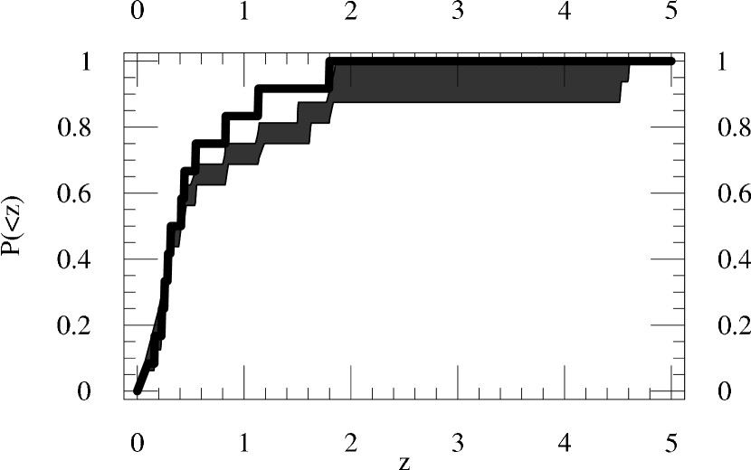
Figure 2.— Cumulative redshift distribution of detected short GRBs. The thick solid curve provides the cumulative distribution of well-constrained GRBs (i.e., the class SH1). The shaded region indicates the range of cumulative distributions produced by assigning redshifts to the weakly-constrained (i.e., the class SH2) in a manner consistent with the constraints. When only an upper or lower limit is available, we pick redshifts using a uniform prior for redshifts between 0 and 5.

2.4. Comparison with prior work

Short GRB interpretation: Several previous efforts have been made to test quantitative MH-based predictions for the host, redshift, luminosity, and age distributions [Meszaros et al. (2006); Guetta & Piran (2006); Nakar et al. (2005); Gal-Yam et al. (2005); Bloom et al. (1999); Belczynski et al. (2006c); Perna & Belczynski (2002)]. However, many authors found puzzling discrepancies; most notably, as has been emphasized by Gal-Yam et al. (2005); Nakar et al. (2005) and by Guetta & Piran (2006) (by comparing redshift-luminosity distributions to models) and as has seemingly been experimentally corroborated with GRB 060502B Bloom et al. (2006a), typical observed short GRBs appear to occur $\approx{\rm(1-few)\times Gyr}$ after their progenitors’ birth. By contrast, most authors expect population synthesis predicts a delay time distribution $dp/dt\propto 1/t$ (e.g., Piran 1992), which was interpreted to imply that short delay times dominate, that DCO mergers occur very soon after birth, and that mergers observed on our light cone predominantly arise from recent star formation. Additionally, on the basis of the observed redshift-luminosity distribution alone, Guetta & Piran (2006) and Nakar et al. (2005) conclude short GRB rates to be at least comparable to observed present-day NS-NS merger rate in the Milky Way. They both also note that a large population of low-luminosity bursts (i.e., $L<10^{49}\,$erg) would remain undetected, a possibility which may have some experimental support: post-facto correlations between short GRBs and nearby galaxies suggests the minimum luminosity of gamma ray bursts ($L_{min}$) could be orders of magnitude lower (Nakar et al., 2005; Tanvir et al., 2005). Such a large population would lead to a discrepancy between the two types of inferred rates. In summary, straightforward studies of the observed SHB sample suggest (i) delay times and (ii) to a lesser extent rate densities are at least marginally and possibly significantly incongruent with the observed present-day Milky Way sample of double NS binaries, and by extension the merger hypothesis (cf. Sections 3.2 and 4 of Nakar et al., 2005). A more recent study by Berger et al. (2006) suggests that high-redshift hosts may be significantly more difficult to identify optically. Using the relatively weak constraints they obtain regarding the redshifts of previously-unidentified bursts, they reanalyze the data to find delay time distributions consistent with $dP/dt\propto 1/t$, as qualitatively expected from detailed evolutionary simulations.

In all cases, however, these comparisons were based on elementary, semianalytic population models, with no prior on the relative likelihood of different models: a model with a Gyr characteristic delay between birth and merger was a priori as likely as $dP/dt\propto 1/t$. For this reason, our study uses a large array of concrete population synthesis simulations, in order to estimate the relative likelihood of different delay time distributions.

Population synthesis: Earlier population synthesis studies have explored similar subject matter, even including heterogeneous galaxy populations (see, e.g. Belczynski et al., 2006c; de Freitas Pacheo et al., 2005; Perna & Belczynski, 2002; Bloom et al., 1999; Fryer et al., 1999; Belczynski et al., 2002a). These studies largely explored a single preferred model, in order to produce what these authors expect as the most likely predictions, such as for the offsets expected from merging supernovae-kicked binaries and the likely gas content of the circumburst environment. Though preliminary short GRB observations appeared to contain an overabundance of short GRBs (Nakar et al., 2005), recent observational analyses such as Berger et al. (2006) suggest high-redshift bursts are also present, in qualitative agreement with the detailed population synthesis study by Belczynski et al. (2006c). The present study quantitatively reinforces this conclusion through carefully reanalyzing the implications of short GRB observations, and particularly through properly accounting for the small short GRB sample size.

The extensive parameter study included here, however, bears closest relation to a similar slightly smaller study in Belczynski et al. (2002a), based on 30 population synthesis models. Though intended for all GRBs, the range of predictions remain highly pertinent for the short GRB population. In most respects this earlier study was much broader than the present work: it examined a much wider range of potential central engines (e.g., white dwarf-black hole mergers) and extracted a wider range of predictions (e.g., offsets from the central host). The present paper, however, not only explores a much larger set of population synthesis models ($\simeq$500) – including an entirely new degree of freedom, the relative proportion of short GRBs hosted in elliptical and spiral galaxies – but also compares predictions specifically against short GRB observations.

3. Other Relevant Observations

3.1. Multicomponent star formation history

The star formation history of the universe has been extensively explored through a variety of methods: extraglactic background light modulo extinction (see,e.g., Nagamine et al., 2006; Hopkins, 2004, and references therein); direct galaxy counts augmented by mass estimates (see,e.g. Bundy et al., 2005, and references therein); galaxy counts augmented with reconstructed star formation histories from their spectral energy distribution (e.g. Heavens et al., 2004; Thompson et al., 2006; Yan et al., 2006; Hanish et al., 2006); and via more general composite methods (Strigari et al., 2005). Since all methods estimate the total mass formed in stars from some detectable quantity, the result depends sensitively on the assumed low-mass IMF and often on extinction. However, as recently demonstrated by Hopkins (2006) and Nagamine et al. (2006), when observations are interpreted in light of a common Chabrier IMF, observations largely converge upon a unique star-formation rate per unit comoving volume $\dot{\rho}=dM/dVdt$ bridging nearby and distant universe, as shown in Figure 3.

Less clearly characterized in the literature are the components of the net star formation history $\dot{\rho}$: the history of star formation in relatively well-defined subpopulations such as elliptical and spiral galaxies. For most of time, galaxies have existed in relatively well-defined populations, with fairly little morphological evolution outside of rare overdense regions (see, e.g. Bundy et al., 2005; Hanish et al., 2006, and references therein). Different populations possess dramatically different histories: the most massive galaxies form most of their stars very early on (see,e.g. Feulner et al., 2005) and hence at a characteristically lower metallicity. Further, as has been extensively advocated by Kroupa (see, e.g. Kroupa & Weidner, 2003; Fardal et al., 2006, and references therein) the most massive structures could conceivably form stars through an entirely different collapse mechanism (“starburst-mode”, driven for example by galaxy collisions and capture) than the throttled mode relevant to disks of spiral galaxies (“disk-mode”), resulting in particular in a different IMF.

Both components significantly influence the present-day merger rate. For example, the initial mass function determines how many progenitors of compact binaries are born from star-forming gas and thus are available to evolve into merging BH-NS or NS-NS binaries. Specifically, as shown in detail in §4.1 and particularly via Figure 4, elliptical galaxies produce roughly three times more high mass binaries per unit mass than their spiral counterparts. Additionally, as first recognized by de Freitas Pacheco et al. (2006), even though elliptical galaxies are quiescent now, the number of compact binaries formed in ellipticals decays roughly logarithmically with time (i.e., $dn/dt\propto 1/t$). Therefore, due to the high star formation rate in elliptical-type galaxies $\sim 10\,{\rm Gyr}$ ago, the star forming mass density $\delta\rho_{e}$ born in ellipticals roughly $t_{e}\sim 10\,{\rm Gyr}$ ago produces mergers at a rate density $\sim\delta\rho_{e}/t_{e}$ that is often comparable to or larger than the rate density of mergers occurring soon after their birth in spiral galaxies $\sim d\rho_{s}/dt$.

Figure 3.— Star formation history of the universe used in this paper. Solid line: Net star formation history implied by Eq. (4). Dashed, dotted line: The star formation history due to elliptical and spiral galaxies, respectively.

3.1.1 Standard two-component model

As a reference model we use the two-component star formation history model presented by Nagamine et al. (2006). This model consists of an early “elliptical” component and a fairly steady “spiral” component, with star formation rates given by

$$\dot{\rho} = \dot{\rho}_{e}+\dot{\rho}_{s}$$ (4)

$$\dot{\rho}_{C} = A_{C}(t/\tau_{C})e^{-t/\tau_{C}}$$ (5)

where cosmological time $t$ is measured starting from the beginning of the universe and where the two components decay timescales are $\tau_{e,s}=$ 1.5 and 4.5 Gyr, respectively (see Section 2 and Table 2 of Nagamine et al., 2006). These normalization constants $A_{e,s}=0.23,0.15M_{\odot}{\rm yr}^{-1}{\rm Mpc}^{-3}$ were chosen by Nagamine et al. (2006) so the integrated amount of elliptical and spiral star formation agrees with (i) the cosmological baryon census [$\Omega_{*}\approx 0.0022$; see Fukugita & Peebles (2004); Read & Trentham (2005) and references therein]; (ii) the expected degree of gas recycling from one generation of stars to the next; and (iii) the relative masses in different morphological components ($60\%:40\%$). Explicitly, these two constants are chosen so $\int\dot{\rho}_{e}/\rho_{c}=\Omega_{*}/0.55\times 0.6$ and $\int\dot{\rho}_{e}/\rho_{c}=\Omega_{*}/0.55\times 0.4$, respectively.

Each component forms stars in its own distinctive conditions, set by comparison with observations of the Milky Way and elliptical galaxies. We assume mass converted into stars in the fairly steady “spiral” component is done so using solar metallicity and with a fixed high-mass IMF power law [$p=-2.7$ in the broken-power-law Kroupa IMF; see Kroupa & Weidner (2003)]. On the other hand, we assume stars born in the “elliptical” component are drawn from a broken power law IMF with high-mass index within $p\in[-2.27,-2.06]$ and metallicity $Z$ within $0.56<Z/Z_{\odot}<2$. These elliptical birth conditions agree with observations of both old ellipticals in the local universe (see Li et al., 2006, and references therein) as well as of young starburst clusters (see Fall et al., 2005; Zhang & Fall, 1999, and references therein).

3.2. Binary pulsar merger rates in the MilkyWay

If binary neutron stars are the source of short GRBs, then the number of short GRBs seen in spirals should be intimately connected to the number of binary pulsars in the Milky Way that are close enough to merge through the emission of gravitational radiation. Four unambiguously merging double pulsars have been found within the Milky Way using pulsar surveys with well-understood selection effects. Kim et al. (2003) developed a statistical method to estimate the likelihood of double neutron star formation rate estimates, designed to account for the small number of known systems and their associated uncertainties. Kalogera et al. (2004) summarize the latest results of this analysis: taking into account the latest pulsar data, a standard pulsar beaming correction factor $f_{b}=6$ for the unknown beaming geometry of PSR J0737–3037, and a likely distribution of pulsars in the galaxy (their model 6), they constrain the rate to be between $r_{\rm MW}=16.9{\rm Myr}^{-1}$ and $292.1{\rm Myr}^{-1}$. ($95\%$ confidence interval).

Assuming all spiral galaxies to form stars similarly to our Milky Way, then the merger rate density in spirals at present ${\cal R}_{{[s]}}(T)$ must agree with the product of the formation rate per galaxy $r_{\rm MW}$ and the density of spiral galaxies $n_{s}$. Based on the ratio of the blue light density of the universe to the blue light attributable to the Milky Way, the density of Milky Way-equivalent galaxies lies between $0.75\times 10^{-2}{\rm Mpc}^{-3}$ and $2\times 10^{-2}{\rm Mpc}^{-3}$ (see Phinney (1991), Kalogera et al. (2001), Nutzman et al. (2004), Kopparapu et al. (2007) and references therein). We therefore expect the merger rate density due to spirals at present to lie between $0.15{\rm Myr}^{-1}{\rm Mpc}^{-3}$ and $5.8{\rm Myr}^{-1}{\rm Mpc}^{-3}$ (with better than 95% confidence).

4. Predictions for Short GRBs

4.1. Population synthesis simulations

We study the formation of compact objects with the StarTrack population synthesis code, first developed by Belczynski et al. (2002b) and recently significantly extended as described in detail in Belczynski et al. (2006a); see §2 of Belczynski et al. (2006b) for a succinct description of the changes between versions.

Since our understanding of the evolution of single and binary stars is incomplete, this code parameterizes several critical physical processes with a great many parameters ($\sim 30$), many of which influence compact-object formation dramatically; this is most typical with all current binary population synthesis codes used by various groups. For the StarTrack population synthesis code, in addition to the IMF and metallicity (which vary depending on whether a binary is born in an elliptical or spiral galaxy), seven parameters strongly influence compact object merger rates: the supernova kick distribution (modeled as the superposition of two independent Maxwellians, using three parameters: one parameter for the probability of drawing from each Maxwellian, and one to characterize the dispersion of each Maxwellian), the solar wind strength, the common-envelope energy transfer efficiency, the fraction of angular momentum lost to infinity in phases of non-conservative mass transfer, and the relative distribution of masses in the binary. Other parameters, such as the fraction of stellar systems which are binary (here, we assume all are, i.e., the binary fraction is equal to $1$) and the distribution of initial binary parameters, are comparatively well-determined (see e.g..Abt (1983), Duquennoy & Mayor (1991) and references therein). Even for the less-well-constrained parameters, some inferences have been drawn from previous studies, either more or less directly (e.g., via observations of pulsar proper motions, which presumably relate closely to supernovae kick strength; see, e.g., Hobbs et al. (2005), Arzoumanian et al. (2002), Faucher-Giguère & Kaspi (2006) and references therein) or via comparison of some subset of binary population synthesis results with observations (e.g., §8 of Belczynski et al. (2006a), van der Sluys et al. (2006), Nelemans & Tout (2005), Willems & Kolb (2002), Podsiadlowski et al. (2002) and references therein). Based on these and other comparisons, while other parameters entering into population synthesis models can influence their results equally strongly, these particular seven parameters are the least constrained observationally. For this reason, despite observational suggestions that point towards preferred values for these seven parameters – and despite the good agreement with short GRB and other observations obtained when using these preferred values (Belczynski et al. (2006c)) – in this paper we will conservatively examine the implications of a plausible range of each of these parameters. More specifically, despite the Milky Way-specific studies of O’Shaughnessy et al. (2005, 2007b) (which apply only to spirals, not the elliptical galaxies included in this paper), in this study we will continue to assume all seven parameters are unknown, drawn from the plausible parameter ranges described in O’Shaughnessy et al. (2007b).

As noted previously in § 3.1, we perform simulations of two different classes of star-forming conditions: “spiral” conditions, with $Z=Z_{\odot}$ and a high-mass IMF slope of $p=-2.7$, and “elliptical” conditions, with a much flatter IMF slope and a range of allowed metallicities $0.56<Z/Z_{\odot}<2$.

Archive selection: Our collection of population synthesis simulations consists of roughly $3000$ and $800$ simulations under spiral and elliptical conditions, respectively. Our archives are highly heterogeneous, with binary sample sizes $N$ that spread over a large range. A significant fraction of the smaller simulations were run with parameters corresponding to low merger rates, and have either no BH-NS or no NS-NS merger events. Therefore, though the set of all population synthesis simulations is unbiased, with each member having randomly distributed model parameters, the set of all simulations with one or more events is slightly biased towards simulations with higher-than-average merger rates. Further, the set of simulations with many events, whose properties (such as the merger rate) can be very accurately estimated, can be very strongly biased towards those models with high merger rates. Fortunately, as discussed at much greater length in the Appendix, the set of simulations with $nN\geq 5\times 10^{6}$ and $n>20$ has small selection bias and enough simulations (976 and 737 simulations NS-NS and BH-NS binaries under spiral-like conditions, as well as 734 and 650 simulations under elliptical conditions, respectively) to explore the full range of population synthesis results, while simultaneously insuring each simulation has enough events to allow us to reliably extract its results.

4.2. Results of simulations

From each population synthesis calculation ($\alpha$) performed under elliptical or spiral conditions ($C=e,s$) and for each final result ($K$), we can estimate: (i) the number of final $K$ events per unit mass of binary mergers progenitors, i.e., the mass efficiency ($\lambda_{C,\alpha,K}$); and (ii) the probability $P_{c,\alpha,K}(<t)$ that given a progenitor of $K$ the event $K$ (e.g., a BH-BH merger) occurs by time $t$ since the formation of $K$. Roughly speaking, for each simulation we take the observed sample of $n$ binary progenitors of $K$, with $M_{1\ldots n}$ and delay times $t_{1\ldots n}$, and estimate

$$\lambda = \frac{n}{N}\frac{f_{cut}}{\left<M\right>}$$ (6)

$$P_{m}(<t) = \sum_{j}\Theta(t-t_{j})$$ (7)

where $\Theta(x)$ is a unit step function; $N$ is the total number of binaries simulated, from which the $n$ progenitors of $K$ were drawn; $\left<M\right>$ is the average mass of all possible binary progenitors; and $f_{cut}$ is a correction factor accounting for the great many very low mass binaries (i.e., with primary mass $m_{1}<m_{c}=4M_{\odot}$) not included in our simulations at all. Expressions for both $\left<M\right>$ and $f_{cut}$ in terms of population synthesis model parameters are provided in Eqs. (1-2) of O’Shaughnessy et al. (2007a). In practice, $P_{m}(t)$ and $dP_{m}/dt$ are estimated with smoothing kernels, as discussed in Appendix B. Given the characteristic sample sizes involved (e.g., $n>200$ for NS-NS), we expect $P_{m}$ to have absolute error less than 0.05 at each point (95% confidence) and $dP_{m}/dt$ to have rms relative error less than 20% (95% confidence). Since these errors are very small in comparison to uncertainties in other quantities in our final calculations (e.g., the star formation rate of the universe), we henceforth ignore errors in $P$ and $dP/dt$.

Figure 4.— Smoothed histograms of the mass efficiency $\lambda$ [Eq. (6)] of simulations used in our calculations, shown for spiral (solid) and elliptical (dotted) birth conditions. As expected given the differences in the IMF, elliptical galaxies produce BH-NS binaries roughly three times more efficiently than spirals. However, apparently because our population synthesis sample involves highly correlated choices for $n$ and $N$ (see the Appendix and Figure 13), our distribution of NS-NS mass efficiencies remains biased, producing identical distributions for both elliptical and spiral birth conditions.

Figures 4, 5, and 6 show explicit results drawn from these calculations. From these figures, we draw the following conclusions:

Uncertainties in binary evolution significantly affect results: As clearly seen by the range of possiblities allowed in Figures 4 and 5, our imperfect understanding of binary evolution implies we must permit and consider models with a wide range of mass efficiencies $\lambda$ and delay time distributions $P_{m}(<t)$.

The merger time distribution is often well-approximated with a one parameter family of distributions, $dP_{m}/dt\propto 1/t$: As suggested by the abundance of near-linear distributions in Figure 5, the delay time distribution $P_{m}$ is almost always linear $\log t$. Further, from the relative infrequency of curve crossings, the slope of $P_{m}$ versus $\log t$ seems nearly constant. As shown in the bottom panels of Figure 6, this constant slope shows up as a strong correlation between the times $t(5\%)$ and $t(50\%)$ at which $P_{m}$ reaches 0.05 and 0.5 when $\log t(5\%)/Myr>1.5$:

$$\log t(50\%)\approx\left\{\begin{array}[]{ll}\log t(5\%)+2.5&\text{if }\log t(5\%)>1.5\\ 10\log t(5\%)-11&\text{if }\log t(5\%)<1.5\end{array}\right.$$ (8)

The merger time distribution is at most weakly correlated with the mass efficiency: Finally, as seen in the top panels of Figure 6, a wide range of efficiencies are consistent with each delay time distribution. The maximum and minmum mass efficiency permitted increase marginally with longer median delay times $t(50\%)$ – roughly an order of magnitude over five orders of magnitude of $t(50\%)$. But to a good approximation, the mass efficiencies and delay times seem to be uncorrelated.

Figure 5.— Cumulative probabilities $P_{m}(<t)$ that a NS-NS binary (left panels) or BH-NS binary (right panels) will merge in time less than $t$, for twenty randomly-chosen population synthesis models, given spiral (top) and elliptical (bottom) star forming conditions. A vertical dashed line indicates the age of the universe. For the sample sizes involved, these distributions are on average accurate to within 0.05 everywhere (with 90% probability); see Figure 14.

Figure 6.— Scatter plots to indicate correlations between results of various simulations. Top panels: Scatter plot of mass efficiency $\log\lambda$ and average delay time $\log t(50\%)$. Bottom panels: Scatter plot of $\log t(5\%)$ versus $\log t(50\%)$; also shown is the analytic estimate of Eq. (8). Left panels indicate spiral conditions; right panels indicate elliptical conditions. Despite the differences between these two types of simulations (i.e., metallicity and initial mass function), the range of delay time distributions and mass efficiencies are largely similar (i.e., the corresponding left and right panels resemble one another).

4.3. Converting simulations to predictions

Each combination of heterogeneous population synthesis model, star formation history, and source model leads to a specific physical signature, embedded in observables such as the relative frequencies with which short GRBs appear in elliptical and spirals, the average age of progenitors in each component, and the observed distribution of sources’ redshifts and luminosities. All of these quantities, in turn, follow from the two functions ${\cal R}_{C}(t)$, the merger rate per unit comoving volume in $C=$ elliptical or spiral galaxies.

The rate of merger events per unit comoving volume is uniquely determined from (i) the SFR of the components of the universe $d\rho_{\{C\}}/dt$; (ii) the mass efficiency $\lambda_{{[C]}}$ at which $K$ mergers occur in each component $C$; and (iii) the probability distribution $dP_{m\{C\}}/dt$ for merger events to occur after a delay time $t$ after star formation:

$${\cal R}(t) = \sum_{C}{\cal R}_{{[C]}}$$ (9)

$${\cal R}_{\{C\}}(t) = \int dt_{b}\lambda_{\{C,K\}}\frac{dP_{m\{C\}}}{dt}(t-t_{b})\frac{d\rho_{\{C\}}}{dt}(t_{b})$$ (10)

Though usually ${\cal R}_{{[C]}}(t)$ is experimentally inaccessible, because our source and detection models treat elliptical and spiral hosts identically, the ratio uniquely determines the fraction $f_{s}$ of spiral hosts at a given redshift:

$$f_{s}(z)={\cal R}_{{[s]}}/({\cal R}_{{[e]}}+{\cal R}_{{[s]}})$$ (11)

Additionally, as described in §3.2 observations of NS-NS in the Milky Way constrain the present-day merger rate of short GRB progenitors (${\cal R}_{{[s]}}(T_{\rm universe})$), if those progenitors are double neutron star binaries.

Unfortunately, the relatively well-understood physical merger rate distributions $R_{{[C]}}$ are disguised by strong observational selection effects described in § 2, notably in the short GRB luminosity function. Based on our canonical source model, we predict the detection rate $R_{D}$ of short GRBs from to be given by

$$R_{D} = \sum_{C}R_{D{[C]}}$$ (12)

$$R_{D{[C]}} = f_{d}^{-1}\int{\cal R}_{{[C]}}P_{[C]}(z)4\pi r^{2}cdt$$

$$\approx \frac{\dot{N}_{min}}{f_{d}f_{b}F_{d}}\int cdt\,\frac{{\cal R}_{{[C]}}(t)}{(1+z)k(z)}$$

where the latter approximation holds for reasonable $\dot{N}_{min}/f_{b}<10^{57}{\rm s}^{-1}$ (i.e., below values corresponding to observed short bursts). While the detection rate depends sensitively on the source and detector models, within the context of our source model the differential redshift distribution $p(z)$

$$p(z)dz \propto \frac{dt}{dz}\sum_{C,K}\frac{{\cal R}_{{[C]}}(t(z))}{(1+z)k(z)}\frac{\dot{N}}{f_{b}}$$ (14)

and the cumulative redshift distribution $P(<z)\equiv\int_{0}^{z}p(z)dz$ do not depend on the source or detector model (Nakar et al., 2005).

Detected luminosity distribution: In order to be self-consistent, the predicted luminosity distribution should agree with the observed peak-flux distribution seen by BATSE. However, so long as $\dot{N}_{min}$ is small for all populations, our hypothesized power-law form $\dot{N}^{-2}$ for the GRB luminosity function immediately implies the detected cumulative peak flux distribution $P(>F)$ is precisely consistent: $P(>F)=(F_{d}/F)$, independent of source population; see for example the discussion in Nakar et al. (2005) near their Eq. (5). While more general source population models produce observed luminosity functions that contain some information about the redshift distribution of bursts – for example, Guetta & Piran (2006) and references therein employ broken power-law luminosity distributions; alternatively, models could introduce correlations between brightness and spectrum – so long as most sources remain unresolved (i.e., small $\dot{N}_{\rm min}$), the observed peak flux distribution largely reflects the intrinsic brightness distribution of sources. Since Nakar et al. (2005) demonstrated this particular brightness distribution corresponds to the observed BATSE flux distribution, we learn nothing new by comparing the observed peak flux distribution with observations and henceforth omit it.

4.4. Predictions for short GRBs

Given two sets of population synthesis model parameters – each of which describe star formation in elliptical and spiral galaxies, respectively – the tools described above provide a way to extract merger and GRB detection rates, assuming all BH-NS or all NS-NS mergers produce (possibly undetected) short GRB events. Rather than explore the (fifteen-dimensional: seven parameters for spirals and eight, including metallicity, for ellipticals) model space exhaustively, we explore a limited array of 500 “model universes” by (i) randomly selecting two population synthesis simulations, one each associated with elliptical ($e$) and spiral ($s$) conditions; (ii) estimating for each simulation the mass efficiency ($\lambda_{e,s}$) and delay time distributions ($P_{e,s}$); (iii) constructing the net merger rate distribution ${\cal R}$ using Eqs. (9,10); and (iv) integrating out the associated expected redshift distribution $p(z)$ [Eq. (14)].

The results of these calculations are presented in Figures 7, 8, 9, 10, and 11. [These figures also compare our calculations’ range of results to observations of short GRBs (summarized in Table 1) and merging Milky Way binary pulsars (Kim et al., 2003); these comparisons will be discussed extensively in the next section.] More specifically, these five figures illustrate the distribution of the following four quantities that we extract from each “model universe”:

Binary merger rates in present-day spiral galaxies: To enable a clear comparison between our multi-component calculations, which include both spiral and elliptical galaxies, and other merger rate estimates that incorporate only present-day star formation in Milky Way-like galaxies, the two solid curves in Figure 7 show the distributions of present-day NS-NS and BH-NS merger rates in spiral galaxies seen in the respective sets of 500 simulations.

In principle, the BH-NS and NS-NS merger rates should be weakly correlated, as the processes (e.g., common envelope) which drive double neutron star to merge also act on low-mass BH-NS binaries, albeit not always similarly; as a trivial example, mass transfer processes that force binaries together more efficiently may deplete the population of NS-NS binaries in earlier evolutionary phases while simultaneously bringing distant BH-NS binaries close enough to merge through gravitational radiation. Thus, a simulation which contains enough BH-NS binaries for us to estimate its delay time distribution $dP/dt$ need not have produced similarly many NS-NS binaries. For this reason, we constructed two independent sets of 500 “model universes”, one each for BH-NS or NS-NS models. However, as a corollary, the randomly-chosen simulations used to construct any given BH-NS “model universe” need not have enough merging NS-NS to enable us to calculate the present-day merger rate, and vice-versa. In particular, we never calculate the double neutron star merger rates in the BH-NS model universe. Thus, though the BH-NS and NS-NS merger rates should exhibit some correlation, we do not explore it here. In particular, in the next section where we compare predictions against observations, we do not require the BH-NS “model universes” reproduce the present-day NS-NS merger rate.

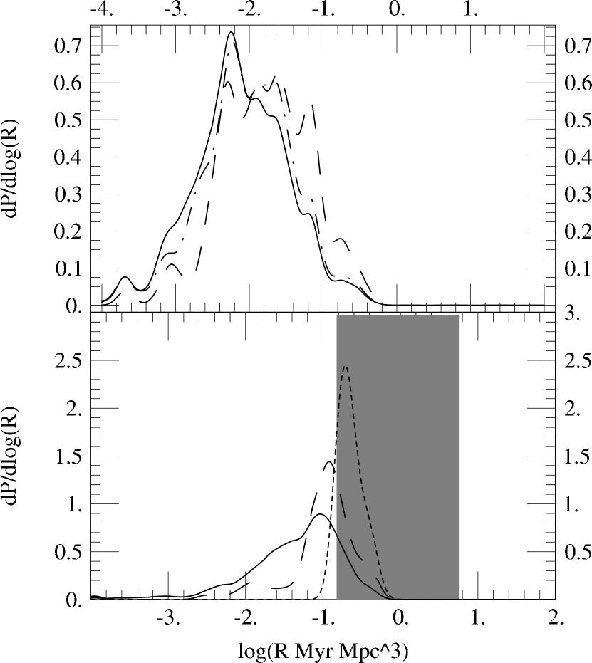
Figure 7.— The distribution of merger rate densities in spiral-type galaxies ${\cal R}_{s}$ for BH-NS mergers (top) and NS-NS mergers (bottom); the solid curve includes all simulations, the dashed curve only those simulations reproducing the observed redshift distribution; and the dotted curve (bottom panel only) only those simulations reproducing the NS-NS merger rate in spiral galaxies derived from an analysis of binary pulsars (also shown on the bottom panel, in gray; see §3.2 for details); and the dot-dashed curve (top panel only) includes only those simulations which, under the most optimistic assumptions, predict short GRBs should occur at least as frequently as has been seen. The bottom panel in particular should be compared with Figure 3 (top panel) of O’Shaughnessy et al. (2007b).

Short GRB detection rate: As described in detail in § 2, the fraction of short GRBs on our past light cone which are not seen depends strongly but simply on unknown factors such as the fraction of bursts pointing towards us, which we characterize by $1/f_{b}$ where $f_{b}$ is the beaming factor, and the fraction of bursts luminous enough to be seen at a given distance, which we characterize by $P(>N_{d})$ where $N_{d}=4\pi r^{2}k(z)(1+z)F_{d}$ is the minimum photon luminosity visible at redshift $z$. The short GRB detection rate also depends on the detector, including the fraction of sky it covers ($1/f_{d}$) and of course the minimum flux $F_{d}$ to which each detector is sensitive. To remove these significant ambiguities, in Figure 8 we use solid curves to plot the distribution of detection rates found for each of our 500 “model universes” (top panel and bottom panel correspond to the BH-NS and NS-NS model universes, respectively), assuming (i) that no burst is less luminous than the least luminous burst seen, namely, GRB 060505, with an apparent (band-limited) isotropic luminosity $\dot{N}_{\rm min\,seen}\simeq 3\times 10^{55}\,{\rm s}^{-1}$, or $L\simeq 7\times 10^{48}\,{\rm erg}\,{\rm s}^{-1}$ (see Table 1); (ii) that beaming has been “corrected”, effectively corresponding to assuming isotropic detector sensitivity and source emission; and (iii) that the detector has a peak flux detection threshold of $F_{d}=1\,{\rm cm}^{-2}\,{\rm s}^{-1}$, corresponding roughly to the true BATSE and Swift peak flux thresholds presented in § 2. These choices are conservative; therefore, our rate estimate for each model universe is an upper bound.

Figure 8.— Distribution of predicted all-sky, beaming-corrected short GRB detection rates $\log R_{D}f_{b}f_{d}$, if bursts arise from BH-NS (top) and NS-NS (bottom) mergers and all bursts produce a higher peak flux of 50-300 keV photons than the least-luminous burst in our sample (with $\dot{N}\simeq 3\times 10^{55}\,{\rm s}^{-1}$), compared to the observed BATSE (dashed vertical line) and Swift (dotted) all-sky detection rate. In other words, a plot of the most optimistic predictions of each two-component “model universe” for the burst detection rate: assuming a detector has all sky visibility, that all burst emit isotropically with no beaming, and that no bursts are faint enough to be missed. Almost all models produce at least as many bursts as are observed; all models can therefore reproduce observations by choosing some low minimum peak photon luminosity $\dot{N}_{\rm min}$, typically $10^{2}$-$10^{3}$ times lower than the one of the faintest burst seen. As in Figure 7, the solid curves include all 500 “model universes”; the dashed curves include only those “model universes” which reproduce the short GRB redshift distribution; the dotted curve (bottom panel only) includes only models which are reasonably consistent with the present-day double neutron star merger rate in the Milky Way; and the dot-dashed curve (top panel only) includes only those simulations which, under the most optimistic assumptions, predict short GRBs should occur at least as frequently as has been seen.

Short GRB redshift distribution: The short GRB detection rate depends on the ability of gamma-ray detectors to distinguish burst events from background noise and the GRB luminosity function. Its selection effects therefore depend only on the properties of gamma-ray telescopes. On the other hand, the short GRB redshift distribution implicitly contains several other selection effects which have not been factored into our analysis (e.g., regarding the availability and reliability of an association of each burst to a host and the ability of optical telescope to extract a spectrum and redshift of that host). Lacking the ability to characterize these selection effects, we perform the most straightforward prediction for the distribution of short GRB redshifts: using Eq. (14), we assume all detected short GRB events have accurate and unambiguous optical follow-up and redshifts. Based upon that assumption, we generate two sets of 500 candidate redshift distributions for short GRBs, assuming either (i) the set of merging BH-NS binaries or (ii) the set of merging NS-NS binaries is identical to (iii) the set of all short GRBs. The results are shown in the top left panels of Figures 9 (for NS-NS binaries) and 10 (for BH-NS binaries). Rather than provide all 500 cumulative redshift distributions, we have sorted these distributions by their value at $z=0.1$ and plotted indicative curves at chosen percentiles: for example, the dotted curves show the 50th and 450th cumulative redshift distributions we obtained, corresponding to the 10th and 90th percentile. Because of the limited number of “model universes” presently available to us, we do not presently attempt to resolve the tails of the distribution; however the range of potential cumulative redshift distributions includes a low a priori probability tail with members which are slightly more biased towards low redshift than the cumulative distributions those shown here.

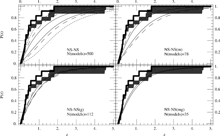
Figure 9.— Demonstration that population synthesis models can reproduce short GRB redshift distributions, assuming NS-NS mergers produce all short GRBs. As in Figure 10, the top right and left panels compare the range of short GRB redshift distributions expected from our two-component model : 1%/99% (dotted), 10%/90% (dashed), and 25%/75% (solid) redshift distributions are overlaid on the observed cumulative redshift distribution, both for all simulated models (top left) and those models which remain everywhere close to the observed redshift distribution (bottom left). Top right: As above, but including only those NS-NS models which produce a NS-NS merger rate in agreement with observations of the Milky Way merger rate (Figure 7). Bottom right: As above, but including only those NS-NS models which reproduce the number of binary pulsars seen in the Milky Way and the short GRB redshift distribution.

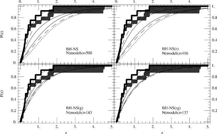
Figure 10.— Demonstration that population synthesis models can reproduce short GRB redshift distributions, assuming BH-NS mergers produce all short GRBs. The jagged curve and shaded regions provide the cumulative redshift distribution for observed short GRBs (Fig. 2). Top left panel: The smooth curves illustrate the range of short GRB redshift distributions; out of the 500 simulated, the two solid curves correspond to the curves with the 25th and 75th percentile values of $P(0.1)$; the dashed curves to the 10th and 90th percentiles; and the dotted curves to the first and 99th percentiles. Bottom left panel: As above, but including only those models which produce redshift distributions which differ from observations by less than $0.38$ (i.e., a 5% Kolmogorov-Smirnov false alarm probability). Top right panel: As previously, but including only those model which, when given the most favorable assumptions, still predict too few short GRB detections. Bottom right panel: As previously, but requiring both the predicted short GRB rate and redshift distribution be simultaneously consistent with GRB observations.

Fraction of mergers in spiral galaxies: Finally, in Figure 11 (solid curves) we show the a priori probability that a fraction $f_{s}$ of binary mergers occur in spiral galaxies, using the scaled variable $X=\text{arctanh}(2f_{s}-1)$. This representation allows us to better illustrate relative probabilities of spiral fractions $f_{s}$ that are very near $1$ or $0$; to give a sense of scale, $X=1(2)$ corresponds to $88\%$ ($98\%$) of all mergers occurring in spiral galaxies.

As seen in Figure 11, a priori we cannot say whether elliptical or spiral galaxies should host most presently-occurring binary mergers. Furthermore, a significant fraction of models have $|X|>1$ (i.e., in those models, almost all mergers occur in spirals or ellipticals). This extreme range for $f_{s}$ can be traced back directly to the large range of mass efficiencies shown in Figure 4. For a randomly chosen pair of population synthesis model for elliptical and spiral galaxies, one will often be significantly larger than the other, leading to a spiral fraction $f_{s}$ near its limits (i.e., $f_{s}\simeq 0,1$).

Figure 11.— Distribution of the fraction of BH-NS mergers (top panel) and NS-NS mergers (bottom panel) expected to occur in spiral galaxies at the present day [Eq. (11) evaluated at $z=0$]. Solid curves include all models; dashed lines include only those models reproducing the redshift distribution; dotted line includes only those models reproducing the merger rate of NS-NS binaries in spiral galaxies, based on the Milky Way; and the dot-dashed line includes only models which could possibly produce as many short GRB events as are observed. To better indicate a very high or very low fraction $f_{s}$ of mergers occurring in spirals, we plot the distributions above versus $X=\tanh^{-1}(2f_{s}-1)$.

5. Testing Predictions Against Observations

To summarize, in this paper we are trying to examine whether either of two very simple hypotheses are consistent with what we have heretofore seen of short GRBs and binary mergers are consistent with our understanding of the star formation history of the universe and of binary stellar evolution. The two simplest hypothesis are, on the one hand, that every short GRB is a binary BH-NS merger and that every BH-NS merger produces a short GRB; and on the other hand the corresponding statement for NS-NS binaries. Further, assuming that in both cases some fraction of all possible models are consistent with observations, we want to understand the properties of those consistent models and the physical processes that require those properties to be as they are. Of course, these comparisons are affected by observational selection effects. Notably, Berger et al. (2006) has suggested that the lack of deep optical follow-up on faint short GRBs has biased the redshift distribution to low redshift. Lacking any ability to control an unknown bias, we proceed with the simplest possible test: we compare existing results to currently known observations. Specifically, we require our predictions for the binary neutron star merger rate (Figure 7, available only for binary neutron star short GRB “model universes”), for the short GRB detection rate (Figure 8), and for the short GRB redshift distribution (Figures 9 and 10) be statistically consistent with the corresponding observations, all of which are shown in their respective plots. We then compare the distribution of constrained quantities (in the aforementioned Figures and in Figures 11 and 12) with their initial distributions, to understand the physics implied by observations.

5.1. Comparisons I: NS-NS as burst source

No definitive evidence exists to determine the fraction of short bursts that are less luminous than the faintest currently known; to discover the degree to which, if any, short GRBs are beamed; and to demonstrate that all mergers must produce bursts. Therefore, we must take the bottom panel of Figure 8 at face value: if no bursts are less luminous than those seen, every short GRB model based on NS-NS produces many more short GRBs than are seen, and therefore every double neutron star “model universe” can reproduce the present-day short GRB detection rate by a proper choice of, for example, the minimum luminosity of short GRBs. Therefore, only two of the three available observations – the short GRB redshift distribution and the set of merging Milky Way binary pulsars – can reject some of the 500 double neutron star “model universes.”

The statistics of this comparison are summarized in Figure 9. Relatively few of our double neutron star models are consistent with observations of merging double pulsars in the Milky Way: 78 out of 500 models, or $\simeq 16\%$; see the top right panel of Figure 9 as well as Figure 7. Among the few models which agree with Milky Way observations, however, most have a cumulative redshift distribution within 0.375 of our family of reference curves and therefore cannot be rejected by a Komolgorov-Smirnov test (95% confidence); see the bottom left panel of Figure 9. Therefore 35 out of 500, roughly $7\%$ of all models, appear fully consistent with all observations considered here and with the assumption that short GRBs are produced exclusively by all NS-NS mergers.

Because observations of the Milky Way suggest a NS-NS merger rate towards the high end of what our simulations produce (see the bottom panel of Fig. 7), and because spiral star formation extends through the recent universe – that is, precisely into the time intervals during which a significant fraction of short GRBs have been observed (see Figure 2) – to an excellent approximation we can conclude that, if short GRBs are due to NS-NS mergers, the best-fitting models of all observations produce mergers and short GRBs preferentially in spiral galaxies, with rapid mergers following quickly upon recent star formation. More specifically, we can generically draw the following explicit conclusions:

High spiral mass efficiency needed: As indicated in Figure 7, only a few populaton synthesis simulations can produce as many merging NS-NS binaries in spiral galaxies as does a natural extrapolation of the known Milky Way NS-NS merger rate. The few “model universes” which reproduce these high merger rates necessarily have non-typical high mass efficiencies $\lambda_{s}$ for forming double neutron stars in spiral galaxies.

High spiral fraction preferred: As a consequence of such high mass efficiencies $\lambda_{s}$ – that is, because of the high rate at which the spiral galaxies in these “universes” produce NS-NS systems – most mergers occur in spirals; equivalently, the spiral fraction $f_{s}$ of constraint-satisfying models is often strongly biased towards spiral galaxies ($f_{s}>1/2$). The bottom panel of Figure 11 explicitly shows that, though unconstrained “universes” can produce mergers preferentially in either elliptical or spiral galaxies (solid curve), in order to reproduce observations of the Milky Way’s merging binary pulsars a “universe” almost always has its mergers predominantly in spirals (dotted curve).

Similarly, since a significant fraction of observed short GRBs are seen at low redshifts (as opposed to during the epoch of elliptical galaxy assembly), spiral-dominated models usually fit observations better than elliptical-dominated ones, as the latter could fit only given an unusually long preferred delay between binary birth and merger. For this reason, demonstrated by the dashed curve in the bottom panel of Figure 11, the “universes” which best fit the short GRB redshift distribution – that is, which have short GRBs occurring relatively recently, during the epoch of spiral star formation – largely produce their short bursts in spiral galaxies.

Low spiral fraction implies long elliptical delays: Conversely, in order for elliptical galaxies to host a significant fraction of mergers, those elliptical galaxies must produce binaries with an unusually long characteristic delay between birth and merger. For example, in the right two panels of Figure 12 compare the prior (top) and constrained (bottom) distribution of spiral fraction and median delay time $t(50\%)$ between birth and merger. As seen in the top panel, the most common delay between birth and merger in a randomly chosen elliptical population synthesis simulation is around $8\,{\rm Gyr}$; however, as seen in the bottom panel, for the handful of “model universes” which have fewer than $80\%$ of double neutron star mergers born in spiral galaxies, the median characteristic delay time is at least an order of magnitude larger.

Figure 12.— A mixed contour and scatter plot of the spiral fraction $f_{s}$ versus the characteristic delay $t(50\%)$ between birth and merger in elliptical galaxies, for BH-NS models (left) and NS-NS models (right). The top panels include all 500 models; the bottom panels provide only those models which satisfy both constraints (for BH-NS simulations, the 137 “model universes” which are consistent with the short GRBs redshift distribution and detection rate; for NS-NS simulations, the 35 “model universes” which are consistent with the short GRB redshift distribution and the number of merging binary neutron stars in the Milky Way). This figure illustrates (i) that the vast majority of constraint-satisfying models have most mergers in spirals [also illustrated in Figure 11] and more critically (ii) that the few models which permit most mergers to occur in elliptical galaxies are slightly biased towards longer characteristic delay times $t(50\%)$.

5.2. Comparisons II: BH-NS as burst source

On the one hand, for purely technical reasons described in § 4 we cannot require our BH-NS “model universes” to be consistent with the present-day NS-NS merger rate. On the other hand, unlike the NS-NS case, a few (84 out of 500) BH-NS “model universes” do predict too few binary mergers to reproduce observations, even given the most optimistic assumptions regarding beaming and the minimum luminosity of short GRBs; see Figure 8. Further, as shown in Figure 10, a significant fraction of redshift distributions (183 out of 500, or $\simeq 37\%$) are consistent with the limited sample, and many of those (137 out of 500, or 27%) are consistent with both the short GRB redshift distribution and detection rate; see Figure 10. From these constraints, we can draw the following conclusions:

Mergers usually in spirals: Just as with NS-NS models, though a priori our “model universes” are equally likely to produce mergers and short GRBs in elliptical and spiral galaxies, the set of “model universes” which reproduce a short GRB redshift distribution that is dominated by recent mergers is biased towards spiral-dominated models: compare the solid and dashed curves in the top panel of Figure 11. However, unlike the NS-NS case where both the redshift distribution (preferring recent star formation) and double neutron star merger rate (requiring very high merger rates in spiral galaxies) limit us to “model universes” that produce extremely many merging binaries, for BH-NS “model universes” only the redshift distribution carries any information that can bias results in favor of spiral galaxies [Fig. 11]. In particular, as illustrated by Figure 7, the distribution of spiral-galaxy BH-NS merger rates remains nearly the same no matter what constraints have been applied.

Ellipticals can be hosts only with significant characteristic delays: Further, as one expects on physical grounds, elliptical galaxies can contain a significant fraction of short GRBs and mergers only when unusually long characteristic delays between birth and merger are involved; see the left two panels of Figure 12.

Unlike the double neutron star case, a significant fraction of “model universes” predict low spiral fractions $f_{s}<0.8$. In order for old elliptical galaxies to host a number of mergers similar to the young spiral galaxies, the binaries in old elliptical galaxies must survive over rather long times – many Gyr after their formation. Comparatively speaking, population synthesis simulations of BH-NS binaries produce more systems with the required characteristic long delay time than do simulations of NS-NS binaries; see for example the fraction of simulations in the top right panels in either Fig. 6 or the top left panel of 12 with $t(50\%)$ greater than $10\,{\rm Gyr}$.

5.3. What fraction of mergers produce short GRBs?

So far, we have required our “model universes” to produce when given the most favorable assumptions regarding burst luminosity distribution and beaming at least as frequent short GRB detections as are observed, as shown in Figure 8. This fairly weak constraint is imposed because, under perfectly plausible but less optimistic assumptions, a great many short GRBs could be missed. However, the difference in Figure 8 between, on the one hand, the vertical lines indicating the observed short GRB detection rate and, on the other hand, an optimistic prediction $f_{d}f_{b}R_{D}$ can be reinterpreted as the fraction of short GRBs that must be missed in order for our predictions to correspond with observations.

By way of example, if a NS-NS “model universe” corresponds to an optimistic detection rate of order $10^{4}\,{\rm yr}^{-1}$, then only $1$ of every 100 NS-NS mergers could produce short GRBs brighter than the least luminous seen and aimed in our direction. This factor of $1/100$ could be produced by any one or combination of several factors, all of which act to decrease the predicted short GRB detection rate below these optimistic predictions: (i) beaming, since the predicted detection rate is proportional to $f_{b}$ and our optimistic calculations assume $f_{b}=1$; (ii) fainter short GRBs, since the detection rate is also proportional to the photon luminosity $\dot{N}_{\rm min}$ of the faintest short burst (i.e., $\propto\dot{N}_{\rm min}/\dot{N}_{\rm min\,seen}$); (iii) some intrinsic physics which prevents all but a select few mergers to produce detectable bursts; or even (iv) further changes in our population synthesis model, such as assuming fewer than 100% (our present choice) of all stars are born in binaries.

No incontrovertible evidence exists that requires any of these factors be less than unity. However, there is good observational and theoretical motivation for re-evaluating our detection rate constraint using a prior on the product of all these factors: essentially, while all could be nearly unity, good reasons exist to imagine that several may be significantly less than 1. For example, (i) Soderberg et al. (2006a) and others have argued that short GRBs may be beamed. Further, (ii) the least luminous burst seen is nearly at our detector’s sensitivity limit, yet short GRBs peak flux distribution is a featureless power law. Since only a remarkable coincidence could produce such a fortuitous combination of detector design and source strength that this burst is indeed at or near the intrinsic burst sensitivity limit, we can reasonably expect the minimum-luminosity burst to be significantly less luminous than the faintest burst yet seen. Additionally, as described in Belczynski et al. (2007), (iii) theoretical simulations of BH-NS mergers could possibly produce short GRB merger events only for a limited array of binary component masses and spins; the fraction of mergers which could be short GRBs ranges from 1/3 to 1/50, depending on the BH birth spin. Finally, (iv) based on comparison with the present-day Milky Way, the binary fraction could be up to a factor two lower than the value we assume; e.g., Belczynski et al. (2007) adopts a binary fraction of 50%. If each of these four factors is decreases the fraction of short GRB detections below our predictions by only factor of roughly $3$, then our expectations for the short GRB detection rate corresponding to a given “model universe” should be lower by nearly a factor of 100!

Adopting a canonical factor of 1/100 to transform the optimistic detection rates presented in Figure 8 into a “realistic” expectations leads to a dramatic transformation of our understanding. On the one hand, extremely few BH-NS “model universes” would produce short GRB events as frequently as are observed. On the other, these “realistic” assumptions cause the 35 constraint-satisfying NS-NS “model universes” to predict roughly as many short GRB events as are observed (i.e., imagine shifting the dotted peak in Figure 8 to the left by 2 orders of magnitude). While this tantalizing correspondance could be a coincidence and while the precise results of our “realistic” prior cannot be taken too seriously, they do remind us of two salient features of our predictions: (i) that BH-NS “model universes” are consistent with the data only given relatively optimistic assumptions, and that they quickly become inconsistent with observations if those assumptions are relaxed; and (ii) that on the other hand because NS-NS “model universes” can allow for so many detections and therefore have much more flexibility in the fraction of short GRBs that are missed, and because double neutron star models are otherwise entirely consistent with all existing observations, double neutron star models for short GRBs remain an attractive candidate explanation for short GRBs.

Comparison to related studies: Belczynski et al. (2007) (hereinafter BTRS) also used the StarTrack population synthesis code and hydrodynamical simulations of BH-NS mergers with BH spins (Rantsiou et al., 2007) to determine whether BH-NS merger events occurred frequently enough, with the right combinations of parameters, to reproduce short GRB observations. In contrast to the present broad study, which relies only on observational constraints, this study adopts several of the “realistic” priors mentioned above to reduce the fraction of merger events that produce short GRBs. Specifically, this paper relies on well-motivated hydrodynamical studies to argue that at best a small fraction of BH-NS mergers ($1/3$ to $1/50$, depending on black hole birth spin) will produce burst events. Additionally, the BTRS simulations rely on a single “most-plausible” set of population synthesis parameters, including in particular a high common envelope efficiency $\alpha\lambda$. As a result, compared to the wide range of common-envelope efficiencies used in this study, BTRS find relatively low BH-NS merger rates. We also note that BTRS assume a 50% binary fraction, lower than the 100% used here. Combining these three factors, BTRS conclude that BH-NS mergers occur too infrequently (less than $10\,{\rm Gpc}^{-3}\,{\rm yr}^{-1}$) to explain short GRB merger rates.

6. Conclusions

In this paper, we used a large archive of concrete, current population synthesis calculations to generate merger rate densities for NS-NS and BH-NS binaries. Using assumptions regarding short GRB source luminosities and detection selection effects, we then compared these rate densities to short GRB detection rates and redshift distributions, as well as to (when available) the present-day Milky Way binary neutron star merger rate. Whether assuming short GRBs arose from either BH-NS mergers or NS-NS mergers, a small but still substantial fraction of models were consistent with existing observations using the most optimistic assumptions for certain priors (i.e., no beaming and all stars born in binaries). Contrary to an earlier study by Nakar et al. (2005), we have demonstrated by using a two-component star formation model that exceptionally long characteristic delays between binary birth and merger are not uniquely required needed to reproduce the short GRB redshift distribution and detection rate, though they are strongly preferred if we additionally demand a significant fraction of short GRBs occur in elliptical hosts. Generally our simulations favor spiral-dominated models: $f_{s}>0.7$. Double neutron star models reproduce observations only if spiral hosts dominate; BH-NS models can permit a wide range of spiral fractions. Though we have not imposed it as a constraint, the fraction of short GRBs in spiral hosts potentially provides an extremely powerful additional constraint on source models. For example, the six host identifications shown in Table 1 suggest the observed spiral fraction $\hat{f}_{s}$ is $50\%$. However, to impose it reliably requires a careful study of the systematic uncertainties in the two-component star formation model used as well as of the selection effects in host galaxy identifications. For example, more massive elliptical galaxies will more efficiently retain any strongly-kicked neutron star binaries but have less gas into which a the short GRB blast wave can collide and produce an afterglow; these and other selection effects

Generally speaking, the exceedingly small number of well-identified short GRBs strongly limits our ability to draw conclusions based on comparisons to properties of that set, such as to the redshift distribution or to the fraction of bursts seen in spiral hosts. More well-identified hosts are needed; additionally, these hosts should hopefully be drawn from a less-biased sample than the present sample appears to be (see Berger et al., 2006). Of course, we encourage deep follow-up searches for afterglows, particularly since our model universes almost always predict a higher proportion of high-redshift short GRBs than has yet been observed. We particularly encourage the development of thorough redshift-limited surveys, since a determination of the relative proportion of bursts in star-forming or elliptical hosts can be done in the nearby universe has significant potential to improve our understanding of the formation mechanism.

Though the limited sample of well-characterized short GRBs currently limits our ability to constrain input physics, we expect that the significant increase in event statistics expected over the next few years will make these events a primary mechanism to constrain double compact object merger rates and the associated astrophysics. For example, with well-understood short GRBs already outnumbering the few known double neutron stars in our galaxy, short GRBs would soon provide the most precise (nonparametric) observational constraint on compact object merger rates (cf Kim et al., 2003), provided the selection effects are quantitatively understood. In turn, these constraints inform us about binary stellar evolution (O’Shaughnessy et al. (2007b),Belczynski et al. (2006a)). Additionally, since short GRB sources would also be copious emitters of gravitational waves, Swift and ground-based gravitational-wave observatories operating in coincidence could conceivably probe the details of an unusually close merger event itself (see,e.g., Kobayashi & Mészáros, 2003; Finn et al., 2004; Nakar et al., 2005). LIGO in particular is both already operating at design sensitivity and conducting triggered searches from GRB observations (Abbott & et al, 2005). Given its compelling qualitative agreement and far-reaching scientific impact, the merger hypothesis deserves a detailed comparison against the best possible models, to either corroborate it, definitively disprove it, or discover weaknesses in our assumptions and models.

Finally, the current sample does not yet allow us to quantify the minimum luminosity and beaming of short GRBs. However assumptions regarding the fraction of merger events which do not produce short GRBs brighter than the weakest burst seen so far and pointing towards us combined with theoretical priors (see,e.g. Belczynski et al., 2007), indicate that BH-NS mergers do not occur frequently enough to explain all short GRBs. We anticipate that future larger samples will allow us to place stronger constraints on the merger models.

Appendix A Archive selection

The predicted short GRB detection rate depends directly on the fraction of star forming mass $\lambda$ predicted to end up in GRB progenitors. However, the mass efficiency $\lambda$ can vary substantially depending on model assumptions. In order to constrain the range of short GRB detection rates expected (for a fixed minimum short GRB luminosity $\dot{N}$), we require the unbiased distributrion of $\lambda$. However, the large variety of simulation sizes in our simulations introduces a bias in our estimate of the mass efficiency distribution – or, equivalently, in the distribution of $n/N$ for $n$ the number of binaries seen and $N$ the number of binaries simulated. Specifically, not all of our archived population synthesis simulations contain enough of each type of event (indexed by $K$) to produce reliable predictions involving it. The set of simulations with $n$ greater than any fixed threshold threshold (including $n=0$) is biased, over-representing simulations with high $n/N$; see for example Figure 13. Since the mass efficiency $\lambda$ is directly proportional to $n/N$ [Eq. (6)], we describe a filter on $n$ and $N$ which preserves the distribution of $n/N$ (for the distribution of $\lambda$) and simultaneously insures that the average simulation has many binaries ($\left<n\right>>200$, so each model’s delay time distribution $dP/dt$ can be accurately estimated).

Formally, each population synthesis simulation converts some unknown fraction $s$ of progenitor binaries into target events $n=sN$. In practice our population sample size $N$ is roughly randomly chosen, independent of the unknown $s$. In other words, we expect the distribution of $n$ and $N$ to derive from two independent distributions for $N$ and $s$, with densities $f$ and $g$:

$$dP(\ln N,\ln n) = f(\ln N)g(\ln(n/N))d\ln Nd\ln n$$ (A1)

$$= f(\ln N)g(\ln n/N)d\ln\sqrt{Nn}d\ln n/N$$

The distribution of $s=n/N$ can be quickly extracted from any two-dimensional distribution in $n,N$ by:

$$gd\ln s=\int\delta\left(\ln(s/(n/N))\right)dP\;.$$ (A2)

However, the above method assumes the distribution perfectly resolved. In practice simulations are generally not repeated, so “fractional” and small $n$ cannot be resolved by repeated trials; instead, only simulations with $s\gg 1/N$ will produce enough events to provide reliable estimates of $s$, and thus its distribution. This truncation effect biases our reconstruction of the two-dimensional density and therefore our reconstruction of the mass efficiency distribution. If we had perfect foreknowledge, however, we could have chosen our sample size so $nN$ was constant and large. Though we would choose $n$ and $N$ in a highly correlated fashion, we would guarantee each point was well-resolved; our method above would correctly reconstruct the distribution of $s$. Hence choosing all population synthesis archives with $nN$ greater than any threshold will allow accurate estimation of the distribution of $s$.

Based on the above discussion and the observed distributions in $n$ and $N$, we introduce cutoffs on $n$ ($>20$) and $nN$ ($>5\times 10^{6}$) which remove the least resolved simulations from consideration (via the $n$ cutoff), reduce the bias associated with a minimum $n$ (via the $nN$ cutoff), and insure that most simulations have at least $200$ binaries (both).

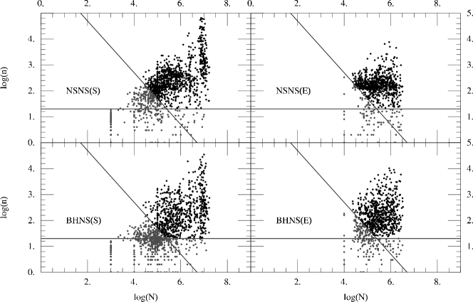
Figure 13.— For spiral (left two panels) and elliptical (right to panels) archives, a scatter plot of the number of NS-NS (top) and BH-NS (bottom) binaries $n$ seen in a simulation of $N$ progenitor binaries (all of $m>4M_{\odot}$, with primary mass drawn from the broken-Kroupa IMF). The two solid lines show the cutoffs $n>20$ and $nN>5\times 10^{6}$ imposed to insure data quality and reduce sampling bias. Simulations used in this paper, shown in black, must lie above and to the right of these cutoffs.

Appendix B Estimating Delay Time Distribution

Poisson errors associated with the limited sample size of our population synthesis simulations inhibits our ability to reconstruct the delay time distribution, whether represented as a cumulative distribution $P_{m}(t)\equiv P_{m}(<t)$, the probability that a delay between birth and merger is less than $t$, or as $dP_{m}/dt$. Using classical statistical methods – see, e.g., Merritt (1994), Thompson & Tapia (1976), and references therein – we smooth the $n$ observed delay times to build our estimates for $P_{m}(t)$ and $dP_{m}/dt$. This appendix briefly reviews those methods and the accuracy of the resulting estimates.

Estimating cumulative distribution: We estimate the cumulative distribution $P(<t)$ for a sample of population synthesis events by a function $\hat{P}(t)$ that smoothes sample dataover a short smoothing length $s$ in $l_{t}\equiv\log_{10}(t/{\rm Myr})$:

$$\hat{P}_{s}(l_{t}) \equiv \sum_{k=1}^{n}\Theta_{s}(l_{t}-l_{t,k})$$ (B1)

$$\Theta_{s}(x) = \frac{1}{2}\left(1+{\rm erf}(x/s\sqrt{2})\right)$$ (B2)

$$s_{1} = \frac{\left[({\rm max}_{k}l_{t,k})-({\rm min}_{k}l_{t,k})\right]}{10n^{0.4}}$$ (B3)

for $n$ the number of events in our population synthesis sample, $k=1\ldots n$ an index over tat same sample, and $l_{t,k}=\log(t_{k}/{\rm Myr})$ the logarithm of the delay $t_{k}$ between binary formation and merger for the $k$th binary. The extremely short smoothing length used here approximately minimizes the average difference between predictions and results.

Figure 14.— Results for errors in estimates of $P(t_{m})$ and $dP_{m}/dt$, versus the number of points used in the estimate, for the trial distribution function $dP_{m}/dt=\frac{0.079}{t}$ between $30$ and $10^{7}\,{\rm Myr}$. Left: Plot of the average and $90\%$ supremum-norm error versus $n$ for $P_{m}(t)$, along with fits to these two quantities (namely, $n^{-0.45}/3$ and $0.7n^{-0.47}$, respectively). Right: Plot of the average and 90% bound on fractional error in $dP_{m}/dt$ versus the number of points available, along with fits to these two quantities (namely, $0.36n^{-0.17}$ and $0.73n^{-0.23}$, respectively).

To test this approach, for several $n$ we drew many Monte Carlo samples of $n$ delay times from a canonical cumulative distribution:

$$P_{m}(l_{t})=\frac{lt-\log(30)}{7-\log(30)}\Theta(l_{t}-\log(30))\Theta(7-l_{t})$$

Figure 14 shows the average and 90% distance ${\rm max}_{l_{t}}|P_{m}(l_{t})-\hat{P}_{m}(l_{t})|$ between our function and our fit versus the number of points smoothed to estimate $P_{m}(t)$.

Given the archive selection procedure presented in A, each archive typically contains of order $n\approx 100$ merging binaries. For such a typical archive, our smoothing method will reconstruct $P(t)$ almost everywhere to better than $5\%$, with the largest errors typically arising near the largest and smallest delay times. As expected, the maximum error agrees perfectly with the distance between observations and data for a Kolmogorov-Smirnov 95% hypothesis test.

Estimating differential distribution : Similarly, we estimate $dP_{m}/dt$ by $\hat{\dot{P}}_{m,10s}$, defined using the time derivative of $P_{m}(<t)$ after converting from logarithmic to physical time:

$$\hat{\dot{P}}_{m} \equiv \frac{1}{t\ln 10}\frac{d\hat{P}_{m}}{dl_{t}}=\frac{1}{t\ln 10}\sum_{k=1}^{n}\frac{1}{\sqrt{2\pi(s_{2})^{2}}}e^{-(\log t-l_{t,k})^{2}/2(s_{2})^{2}}$$ (B4)

$$s_{2} \equiv \frac{\left[({\rm max}_{k}l_{t,k})-({\rm min}_{k}l_{t,k})\right]}{1.25\sqrt{n}}$$ (B5)

Compared to the previous case of estimating the cumulative distribution $P_{m}(t)$, where a significant fraction of all sampled points affect the estimate at any $t$, a significantly longer smoothing length $s_{2}$ is required to estimate $dP_{m}/dt$, since roughly only those few sample points within $s_{2}$ of $t$ contribute to our estimate. As a result, we cannot confidently estimate $dP_{m}/dt$ more accurately than $\approx 30\%$.

To demonstrate that smoothing produces a fairly inaccurate prediction for $dP_{m}/dt$, we applied it to the trial problem mentioned above. To estimate the mean relative error $I$ associated with our estimate in the physically pertinent interval of roughly $100$ Myr to $15$ Gyr by

$$I \equiv \left[\int_{1.8}^{4.5}\frac{dl_{t}}{2.7}\frac{|\hat{\dot{P}}-\dot{P}|^{2}}{(\hat{\dot{P}}^{2}+\dot{P}^{2})/2}\right]^{1/2}\;,$$ (B6)

which generalizes an rms measurement of the relative error in $P$ to allow for large relative errors [i.e., when $\hat{\dot{P}}_{m}=\dot{P}_{m}(1+\delta(l_{t}))$, then $I=(\int\delta^{2}dl_{t}/\Delta l_{t})^{1/2}$]. The second panel of Figure 14 demonstrates that large errors are inevitable, even with many sample points and using a smoothing length $s_{2}$ which is approximately optimized for each $n$. While this slow convergence is a familiar problem for all density estimators (see,e.g. Thompson & Tapia, 1976), it severely limits the ability of any population synthesis simulation to reliable estimate $dP_{m}/dt$, given the severe computational limits involved. By way of example, a delay time distribution accurate to $5\%$ would require roughly $6^{4}\approx 1300$ times more binaries than a $30\%$ accurate estimate.

Implications for short GRB predictions: The short GRB detection rate, redshift distribution, and elliptical-to-spiral ratio all depend on estimates of $dP_{m}/dt$. However, while our reconstruction of $dP_{m}/dt$ for any fixed population synthesis model involves substantial uncertainties, these are not much greater than our corresponding uncertainty in our estimate of that model’s the mass efficiency $\lambda$. Further, these uncertainties are vastly less than the systematic uncertainty involved in not knowing the physically appropriate population synthesis model (i.e., roughly two orders of magnitude uncertainty in $\lambda$).

References

- Abbott & et al (2005) Abbott, B. & et al. 2005, Phys. Rev. D, 72, 042002 [ADS]
- Abt (1983) Abt, H. A. 1983, ARA&A, 21, 343 [ADS]
- Ando (2004) Ando, S. 2004, Journal of Cosmology and Astro-Particle Physics, 6, 7 [ADS]
- Arzoumanian et al. (2002) Arzoumanian, Z., Chernoff, D. F., & Cordes, J. M. 2002, ApJ, 568, 289 [ADS]
- Barthelmy et al. (2005) Barthelmy, S. D., Chincarini, G., Burrows, D. N., Gehrels, N., Covino, S., Moretti, A., Romano, P., O’Brien, P. T., Sarazin, C. L., Kouveliotou, C., Goad, M., Vaughan, S., Tagliaferri, G., Zhang, B., Antonelli, L. A., Campana, S., Cummings, J. R., D’Avanzo, P., Davies, M. B., Giommi, P., Grupe, D., Kaneko, Y., Kennea, J. A., King, A., Kobayashi, S., Melandri, A., Meszaros, P., Nousek, J. A., Patel, S., Sakamoto, T., & Wijers, R. A. M. J. 2005, Nature, 438, 994 [ADS]
- Belczynski et al. (2002a) Belczynski, K., Bulik, T., & Rudak, B. 2002a, ApJ, 571, 394 [ADS]
- Belczynski et al. (2002b) Belczynski, K., Kalogera, V., & Bulik, T. 2002b, ApJ, 572, 407 [ADS]
- Belczynski et al. (2006a) Belczynski, K., Kalogera, V., Rasio, F., Taam, R., Zezas, A., Maccarone, T., & Ivanova, N. 2006a, ApJS, in press URL
- Belczynski et al. (2006b) Belczynski, K., Kalogera, V., Rasio, F. A., Taam, R. E., & Bulik, T. 2006b, ArXiv Astrophysics e-prints [ADS]
- Belczynski et al. (2006c) Belczynski, K., Perna, R., Bulik, T., Kalogera, V., Ivanova, N., & Lamb, D. Q. 2006c, ApJ, 648, 1110 [ADS]
- Belczynski et al. (2007) Belczynski, K., Taam, R. E., Rantsiou, E., & Sluys, M. v. d. 2007, submitted to ApJ (astro-ph/0703131) URL
- Berger (2006) Berger, E. 2006, ArXiv Astrophysics e-prints [ADS]
- Berger (2007) —. 2007, Submitted to ApJ (astro-ph/0702694) URL
- Berger et al. (2006) Berger, E., Fox, D. B., Price, P. A., Nakar, E. a d Gal-Yam, A., Holz, D. E., Schmidt, B. P., Cucchiara, A., Cenko, S. B., Kulkarni, S. R., Soderberg, A. M., Frail, D. A., Penprase, B. E., Rau, A., Ofek, E., Burnell, S. J. B., Cameron, P. B., Cowie, L. L., Dopita, M. A., Hook, I., Peterson, B. A., Podsiadlowski, P., Roth, K. C., Rutledge, R. E., Sheppard, S. S., & Songaila, A. 2006, Submitted to ApJ (astro-ph/0611128) URL
- Berger et al. (2005a) Berger, E., Kulkarni, S. R., Fox, D. B., Soderberg, A. M., Harrison, F. A., Nakar, E., Kelson, D. D., Gladders, M. D., Mulchaey, J. S., Oemler, A., Dressler, A., Cenko, S. B., Price, P. A., Schmidt, B. P., Frail, D. A., Morrell, N., Gonzalez, S., Krzeminski, W., Sari, R., Gal-Yam, A., Moon, D.-S., Penprase, B. E., Jayawardhana, R., Scholz, A., Rich, J., Peterson, B. A., Anderson, G., McNaught, R., Minezaki, T., Yoshii, Y., Cowie, L. L., & Pimbblet, K. 2005a, ApJ, 634, 501 [ADS]
- Berger et al. (2005b) Berger, E., Price, P. A., Cenko, S. B., Gal-Yam, A., Soderberg, A. M., Kasliwal, M., Leonard, D. C., Cameron, P. B., Frail, D. A., Kulkarni, S. R., Murphy, D. C., Krzeminski, W., Piran, T., Lee, B. L., Roth, K. C., Moon, D.-S., Fox, D. B., Harrison, F. A., Persson, S. E., Schmidt, B. P., Penprase, B. E., Rich, J., Peterson, B. A., & Cowie, L. L. 2005b, Nature, 438, 988 [ADS]
- Bloom et al. (2006a) Bloom, J. S., Perley, D. A., Chen, H. ., Butler, N., Prochaska, J. X., Kocevski, D., Blake, C. H., Szentgyorgyi, A., & Falco, E. E. 2006a, ArXiv Astrophysics e-prints [ADS]
- Bloom et al. (2006b) Bloom, J. S., Prochaska, J. X., Pooley, D., Blake, C. H., Foley, R. J., Jha, S., Ramirez-Ruiz, E., Granot, J., Filippenko, A. V., Sigurdsson, S., Barth, A. J., Chen, H.-W., Cooper, M. C., Falco, E. E., Gal, R. R., Gerke, B. F., Gladders, M. D., Greene, J. E., Hennanwi, J., Ho, L. C., Hurley, K., Koester, B. P., Li, W., Lubin, L., Newman, J., Perley, D. A., Squires, G. K., & Wood-Vasey, W. M. 2006b, ApJ, 638, 354 [ADS]
- Bloom et al. (1999) Bloom, J. S., Sigurdsson, S., & Pols, O. R. 1999, MNRAS, 305, 763 URL
- Bundy et al. (2005) Bundy, K., Ellis, R. S., & Conselice, C. J. 2005, ApJ, 625, 621 [ADS]
- Campana et al. (2006) Campana, S., Tagliaferri, G., Lazzati, D., Chincarini, G., Covino, S., Page, K., Romano, P., Moretti, A., Cusumano, G., Mangano, V., Mineo, T., La Parola, V., Giommi, P., Perri, M., Capalbi, M., Zhang, B., Barthelmy, S., Cummings, J., Sakamoto, T., Burrows, D. N., Kennea, J. A., Nousek, J. A., Osborne, J. P., O’Brien, P. T., Godet, O., & Gehrels, N. 2006, A&A, 454, 113 [ADS]
- Che et al. (1999) Che, H., Yang, Y., & Nemiroff, R. J. 1999, ApJ, 516, 559 [ADS]
- Covino et al. (2006) Covino, S., Malesani, D., Israel, G. L., D’Avanzo, P., Antonelli, L. A., Chincarini, G., Fugazza, D., Conciatore, M. L., Della Valle, M., Fiore, F., Guetta, D., Hurley, K., Lazzati, D., Stella, L., Tagliaferri, G., Vietri, M., Campana, S., Burrows, D. N., D’Elia, V., Filliatre, P., Gehrels, N., Goldoni, P., Melandri, A., Mereghetti, S., Mirabel, I. F., Moretti, A., Nousek, J., O’Brien, P. T., Pellizza, L. J., Perna, R., Piranomonte, S., Romano, P., & Zerbi, F. M. 2006, A&A, 447, L5 [ADS]
- de Freitas Pacheco et al. (2006) de Freitas Pacheco, J. A., Regimbau, T., Vincent, S., & Spallicci, A. 2006, International Journal of Modern Physics D, 15, 235 [ADS] [ADS]
- de Freitas Pacheo et al. (2005) de Freitas Pacheo, J. A., Regimbau, T., Vincent, T., & Spallici, A. 2005, IJMPD, In press URL
- de Ugarte Postigo et al. (2006) de Ugarte Postigo, A., Castro-Tirado, A. J., Guziy, S., Gorosabel, J., Johannesson, G., Aloy, M. A., McBreen, S., Lamb, D. Q., Benitez, N., Jelinek, M., Pandey, S. B., Coe, D., Perez-Ramirez, M. D., Aceituno, F. J., Alises, M., Acosta-Pulido, J. A., Gomez, G., Lopez, R., Donaghy, T. Q., Nakagawa, Y. E., Sakamoto, T., Ricker, G. R., Hearty, F. R., Bayliss, M., Gyuk, G., & York, D. G. 2006, ArXiv Astrophysics e-prints [ADS]
- Dietz (2006) Dietz, A. 2006 URL
- Donaghy et al. (2006) Donaghy, T. Q., Lamb, D. Q., Sakamoto, T., Norris, J. P., Nakagawa, Y., Villasenor, J., Atteia, J. ., Vanderspek, R., Graziani, C., Kawai, N., Ricker, G. R., Crew, G. B., Doty, J., Prigozhin, G., Jernigan, J. G., Shirasaki, Y., Suzuki, M., Butler, N., Hurley, K., Tamagawa, T., Yoshida, A., Matsuoka, M., Fenimore, E. E., Galassi, M., Boer, M., Dezalay, J. ., Olive, J. ., Levine, A., Martel, F., Morgan, E., Sato, R., Woosley, S. E., Braga, J., Manchanda, R., Pizzichini, G., Takagishi, K., & Yamauchi, M. 2006, ArXiv Astrophysics e-prints [ADS]
- Duquennoy & Mayor (1991) Duquennoy, A. & Mayor, M. 1991, A&A, 248, 485 [ADS]
- Fall et al. (2005) Fall, S. M., Chandar, R., & Whitmore, B. C. 2005, ApJ, 631, L133 [ADS]
- Fardal et al. (2006) Fardal, M. A., Katz, N., Weinberg, D. H., & Dav’e, R. 2006, ArXiv Astrophysics e-prints [ADS]
- Faucher-Giguère & Kaspi (2006) Faucher-Giguère, C.-A. & Kaspi, V. M. 2006, ApJ, 643, 332 [ADS]
- Feulner et al. (2005) Feulner, G., Gabasch, A., Salvato, M., Drory, N., Hopp, U., & Bender, R. 2005, ApJ, 633, L9 [ADS]
- Finn et al. (2004) Finn, L. S., Krishnan, B., & Sutton, P. J. 2004, ApJ, 607, 384 [ADS]
- Fox et al. (2005) Fox, D. B., Frail, D. A., Price, P. A., Kulkarni, S. R., Berger, E., Piran, T., Soderberg, A. M., Cenko, S. B., Cameron, P. B., Gal-Yam, A., Kasliwal, M. M., Moon, D.-S., Harrison, F. A., Nakar, E., Schmidt, B. P., Penprase, B., Chevalier, R. A., Kumar, P., Roth, K., Watson, D., Lee, B. L., Shectman, S., Phillips, M. M., Roth, M., McCarthy, P. J., Rauch, M., Cowie, L., Peterson, B. A., Rich, J., Kawai, N., Aoki, K., Kosugi, G., Totani, T., Park, H.-S., MacFadyen, A., & Hurley, K. C. 2005, Nature, 437, 845 [ADS]
- Fryer et al. (1999) Fryer, C. L., Woosley, S. E., & Hartmann, D. H. 1999, ApJ, 526, 152 [ADS]
- Fukugita & Peebles (2004) Fukugita, M. & Peebles, P. J. E. 2004, ApJ, 616, 643 [ADS]
- Gal-Yam et al. (2005) Gal-Yam, A., Nakar, E., Ofek, E., Fox, D. B., Cenko, S. B., Kulkarni, S. R., Soderberg, A. M., Harrison, F., Price, P. A., Penprase, B. E., Frail, D., Berger, E., Gladders, M., & Mulchaey, J. 2005, ArXiv Astrophysics e-prints [ADS]
- Gehrels et al. (2007) Gehrels, N., Cannizzo, J. K., & Norris, J. P. 2007, New Journal of Physics, 9, 37 [ADS]
- Gehrels et al. (2005) Gehrels, N., Sarazin, C. L., O’Brien, P. T., Zhang, B., Barbier, L., Barthelmy, S. D., Blustin, A., Burrows, D. N., Cannizzo, J., Cummings, J. R., Goad, M., Holland, S. T., Hurkett, C. P., Kennea, J. A., Levan, A., Markwardt, C. B., Mason, K. O., Meszaros, P., Page, M., Palmer, D. M., Rol, E., Sakamoto, T., Willingale, R., Angelini, L., Beardmore, A., Boyd, P. T., Breeveld, A., Campana, S., Chester, M. M., Chincarini, G., Cominsky, L. R., Cusumano, G., de Pasquale, M., Fenimore, E. E., Giommi, P., Gronwall, C., Grupe, D., Hill, J. E., Hinshaw, D., Hjorth, J., Hullinger, D., Hurley, K. C., Klose, S., Kobayashi, S., Kouveliotou, C., Krimm, H. A., Mangano, V., Marshall, F. E., McGowan, K., Moretti, A., Mushotzky, R. F., Nakazawa, K., Norris, J. P., Nousek, J. A., Osborne, J. P., Page, K., Parsons, A. M., Patel, S., Perri, M., Poole, T., Romano, P., Roming, P. W. A., Rosen, S., Sato, G., Schady, P., Smale, A. P., Sollerman, J., Starling, R., Still, M., Suzuki, M., Tagliaferri, G., Takahashi, T., Tashiro, M., Tueller, J., Wells, A. A., White, N. E., & Wijers, R. A. M. J. 2005, Nature, 437, 851 [ADS]
- Ghirlanda et al. (2004) Ghirlanda, G., Ghisellini, G., & Celotti, A. 2004, A&A, 422, L55 [ADS]
- Grupe et al. (2006a) Grupe, D., Burrows, D. N., Patel, S. K., Kouveliotou, C., Zhang, B., Meszaros, P., Wijers, R. A. M., & Gehrels, N. 2006a, ArXiv Astrophysics e-prints [ADS]
- Grupe et al. (2006b) Grupe, D., Burrows, D. N., Patel, S. K., Kouveliotou, C., Zhang, B., Mészáros, P., Wijers, R. A. M., & Gehrels, N. 2006b, ApJ, 653, 462 [ADS]
- Guetta & Piran (2005) Guetta, D. & Piran, T. 2005, A&A, 435, 421 [ADS]
- Guetta & Piran (2006) —. 2006, A&A, 453, 823 [ADS] [ADS]
- Hakkila et al. (2003) Hakkila, J., Giblin, T. W., Roiger, R. J., Haglin, D. J., Paciesas, W. S., & Meegan, C. A. 2003, ApJ, 582, 320 [ADS]
- Hakkila et al. (1997) Hakkila, J., Meegan, C. A., Pendleton, G. N., Henze, W., McCollough, M., Kommers, J. M., & Briggs, M. S. 1997, To appear in the Fourth Huntsville Gamma-Ray Burst Symposium (astro-ph/9712091) URL
- Hanish et al. (2006) Hanish, D. J., Meurer, G. R., Ferguson, H. C., Zwaan, M. A., Heckman, T. M., Staveley-Smith, L., Bland-Hawthorn, J., Kilborn, V. A., Koribalski, B. S., Putman, M. E., Ryan-Weber, E. V., Oey, M. S., Kennicutt, R. C., Jr., Knezek, P. M., Meyer, M. J., Smith, R. C., Webster, R. L., Dopita, M. A., Doyle, M. T., Drinkwater, M. J., Freeman, K. C., & Werk, J. K. 2006, ArXiv Astrophysics e-prints [ADS]
- Heavens et al. (2004) Heavens, A., Panter, B., Jimenez, R., & Dunlop, J. 2004, Nature, 428, 625 [ADS]
- Hobbs et al. (2005) Hobbs, G., Lorimer, D. R., Lyne, A. G., & Kramer, M. 2005, MNRAS, 360, 974 [ADS]
- Hopkins (2004) Hopkins, A. M. 2004, ApJ, 615, 209 [ADS]
- Hopkins (2006) —. 2006, to appear in the proceedings of ’At the Edge of the Universe’ (astro-ph/0611283) URL
- Kalogera et al. (2004) Kalogera, V., Kim, C., Lorimer, D. R., Burgay, M., D’Amico, N., Possenti, A., Manchester, R. N., Lyne, A. G., Joshi, B. C., McLaughlin, M. A., Kramer, M., Sarkissian, J. M., & Camilo, F. 2004, ApJ, 614, L137 [ADS]
- Kalogera et al. (2001) Kalogera, V., Narayan, R., Spergel, D. N., & Taylor, J. H. 2001, ApJ, 556, 340 URL
- Kim et al. (2003) Kim, C., Kalogera, V., & Lorimer, D. R. 2003, ApJ, 584, 985 [ADS]
- Kim et al. (2006) Kim, C., Kalogera, V., & Lorimer, D. R. 2006, in A life with stars URL
- Kobayashi & Mészáros (2003) Kobayashi, S. & Mészáros, P. 2003, ApJ, 589, 861 [ADS]
- Kopparapu et al. (2007) Kopparapu, R. K., Hanna, C. R., Kalogera, V., O’Shaughnessy, R., Gonzalez, G., Brady, P. R., & Fairhurst, S. 2007, (arXiv:0706.1283) URL
- Kouveliotou et al. (1993) Kouveliotou, C., Meegan, C. A., Fishman, G. J., Bhat, N. P., Briggs, M. S., Koshut, T. M., Paciesas, W. S., & Pendleton, G. N. 1993, ApJ, 413, L101 [ADS]
- Kroupa & Weidner (2003) Kroupa, P. & Weidner, C. 2003, ApJ, 598, 1076 URL
- La Parola et al. (2006) La Parola, V., Mangano, V., Fox, D., Zhang, B., Krimm, H. A., Cusumano, G., Mineo, T., Burrows, D. N., Barthelmy, S., Campana, S., Capalbi, M., Chincarini, G., Gehrels, N., Giommi, P., Marshall, F. E., Mészáros, P., Moretti, A., O’Brien, P. T., Palmer, D. M., Perri, M., Romano, P., & Tagliaferri, G. 2006, A&A, 454, 753 [ADS]
- Lazzati et al. (2005) Lazzati, D., Ghirlanda, G., & Ghisellini, G. 2005, MNRAS, 362, L8 [ADS]
- Lee et al. (2005) Lee, W. H., Ramirez-Ruiz, E., & Granot, J. 2005, ApJ, 630, L165 [ADS]
- Levan et al. (2006) Levan, A. J., Tanvir, N. R., Fruchter, A. S., Rol, E., Fynbo, J. P. U., Hjorth, J., Williams, G., Bergeron, E., Bersier, D., Bremer, M., Grav, T., Jakobsson, P., Nilsson, K., Olszewski, E., Priddey, R. S., Rafferty, D., & Rhoads, J. 2006, ApJ, 648, L9 [ADS]
- Li et al. (2006) Li, Z., Zhang, F., & Han, Z. 2006, accepted for publication to ChJAA (astro-ph/0605610) URL
- Merritt (1994) Merritt, D. 1994 [ADS]
- Meszaros et al. (2006) Meszaros, A., Bagoly, Z., Balazs, L. G., & Horvath, I. 2006, accepted for publication in A andA (astro-ph/0606377) URL
- Nagamine et al. (2006) Nagamine, K., Ostriker, J. P., Fukugita, M., & Cen, R. 2006, ApJ, 653, 881 URL [ADS]
- Nakar (2007) Nakar, E. 2007, ArXiv Astrophysics e-prints [ADS]
- Nakar et al. (2005) Nakar, E., Gal-Yam, A., & Fox, D. 2005, ApJ (in press) URL
- Nakar et al. (2006) Nakar, E., Gal-Yam, A., Piran, T., & Fox, D. B. 2006, ApJ, 640, 849 [ADS]
- Nelemans & Tout (2005) Nelemans, G. & Tout, C. A. 2005, MNRAS, 356, 753 [ADS]
- Norris & Bonnell (2006) Norris, J. P. & Bonnell, J. T. 2006, ApJ, 643, 266 [ADS]
- Nutzman et al. (2004) Nutzman, P., Kalogera, V., Finn, L. S., Hendrickson, C., & Belczynski, K. 2004, ApJ, 612, 364 [ADS]
- Ofek et al. (2007) Ofek, E. O., Cenko, S. B., Gal-Yam, A., Fox, D. B., Nakar, E., Rau, A., Frail, D. A., Kulkarni, S. R., Price, P. A., Schmidt, B. P., Soderberg, A. M., Peterson, B., Berger, E., Sharon, K., Shemmer, O., Penprase, B. E., Chevalier, R. A., Brown, P. J., Burrows, D. N., Gehrels, N., Harrison, F., Holland, S. T., Mangano, V., McCarthy, P. J., Moon, D. S., Nousek, J. A., Persson, S. E., Piran, T., & Sari, R. 2007, ApJ submitted (astro-ph/0703192) URL
- O’Shaughnessy et al. (2007a) O’Shaughnessy, R., Kalogera, V., & Belczynski, K. 2007a, ApJ, 667, 1048 URL
- O’Shaughnessy et al. (2005) O’Shaughnessy, R., Kim, C., Fragos, T., Kalogera, V., & Belczynski, K. 2005, ApJ, 633, 1076 [ADS] [ADS]
- O’Shaughnessy et al. (2007b) O’Shaughnessy, R., Kim, C., Kalogera, V., & Belczynski, K. 2007b, Accepted for publication in ApJ (astro-ph/0610076) URL
- O’Shaughnessy et al. (2007c) O’Shaughnessy, R., O’Leary, R., & Rasio, F. A. 2007c, Phys. Rev. D, 76, 061504 URL
- Paciesas et al. (1999) Paciesas, W. S., Meegan, C. A., Pendleton, G. N., Briggs, M. S., Kouveliotou, C., Koshut, T. M., Lestrade, J. P., McCollough, M. L., Brainerd, J. J., Hakkila, J., Henze, W., Preece, R. D., Connaughton, V., Kippen, R. M., Mallozzi, R. S., Fishman, G. J., Richardson, G. A., & Sahi, M. 1999, ApJS, 122, 465 [ADS]
- Paczynski (1986) Paczynski, B. 1986, ApJ, 308, L43 [ADS]
- Page et al. (2006) Page, K. L., King, A. R., Levan, A. J., O’Brien, P. T., Osborne, J. P., Barthelmy, S. D., Beardmore, A. P., Burrows, D. N., Campana, S., Gehrels, N., Graham, J., Goad, M. R., Godet, O., Kaneko, Y., Kennea, J. A., Markwardt, C. B., Reichart, D. E., Sakamoto, T., & Tanvir, N. R. 2006, ApJ, 637, L13 [ADS]
- Pedersen et al. (2005) Pedersen, K., Elíasdóttir, Á., Hjorth, J., Starling, R., Cerón, J. M. C., Fynbo, J. P. U., Gorosabel, J., Jakobsson, P., Sollerman, J., & Watson, D. 2005, ApJ, 634, L17 [ADS]
- Perna & Belczynski (2002) Perna, R. & Belczynski, K. 2002, Astrophysical Journal, 570, 252 URL
- Phinney (1991) Phinney, E. S. 1991, ApJ, 380, L17 [ADS]
- Podsiadlowski et al. (2002) Podsiadlowski, P., Rappaport, S., & Pfahl, E. D. 2002, ApJ, 565, 1107 [ADS]
- Popov & Stern (2006) Popov, S. B. & Stern, B. E. 2006, MNRAS, 365, 885 [ADS]
- Porciani & Madau (2001) Porciani, C. & Madau, P. 2001, ApJ, 548, 522 [ADS]
- Prochaska et al. (2006) Prochaska, J. X., Bloom, J. S., Chen, H.-W., Foley, R. J., Perley, D. A., Ramirez-Ruiz, E., Granot, J., Lee, W. H., Pooley, D., Alatalo, K., Hurley, K., Cooper, M. C., Dupree, A. K., Gerke, B. F., Hansen, B. M. S., Kalirai, J. S., Newman, J. A., Rich, R. M., Richer, H., Stanford, S. A., Stern, D., & van Breugel, W. J. M. 2006, ApJ, 642, 989 [ADS]
- Rantsiou et al. (2007) Rantsiou, E., Kobayashi, S., Laguna, P., & Rasio, F. 2007, ArXiv Astrophysics e-prints [ADS]
- Read & Trentham (2005) Read, J. I. & Trentham, N. 2005, Royal Society of London Philosophical Transactions Series A, 363, 2693 [ADS]
- Roming (2005) Roming, P. 2005, arxiv eprints URL
- Schmidt (1999) Schmidt, M. 1999, ApJ, 523, L117 [ADS]
- Schmidt (2001) —. 2001, ApJ, 552, 36 [ADS]
- Soderberg et al. (2006a) Soderberg, A. M., Berger, E., Kasliwal, M., Frail, D. A., Price, P. A., Schmidt, B. P., Kulkarni, S. R., Fox, D. B., Cenko, S. B., Gal-Yam, A., Nakar, E., & Roth, K. C. 2006a, ArXiv Astrophysics e-prints [ADS]
- Soderberg et al. (2006b) —. 2006b, ApJ, 650, 261 [ADS]
- Strigari et al. (2005) Strigari, L. E., Beacom, J. F., Walker, T. P., & Zhang, P. 2005, Journal of Cosmology and Astro-Particle Physics, 4, 17 [ADS]
- Tanvir et al. (2005) Tanvir, N. R., Chapman, R., Levan, A. J., & Priddey, R. S. 2005, Nature, 438, 991 [ADS]
- Thoene et al. (2007) Thoene, C. C., Fynbo, J. P. U., Oestlin, G., Milva g-Jensen, B., Wiersema, K., Malesani, D., Ferreira, D. D. M. an Gorosabel, J., Kann, D. A., Watson, D., Michalowski, M. J. an Hjorth, J., Fruchter, A. S., & Sollerman, J. 2007, submitted to ApJ (astro-ph/0703407) URL
- Thompson & Tapia (1976) Thompson, J. & Tapia, R. 1976, Nonparametric function estimation, modelling, and simulation ( Society for Industrial and Applied Mathematics)
- Thompson et al. (2006) Thompson, R. I., Eisenstein, D., Fan, X., Dickinson, M., Illingworth, G., & Kennicutt, R. C. 2006, ArXiv Astrophysics e-prints [ADS]
- van der Sluys et al. (2006) van der Sluys, M. V., Verbunt, F., & Pols, O. R. 2006, A&A, 460, 209 [ADS]
- Villasenor et al. (2005) Villasenor, J. S., Lamb, D. Q., Ricker, G. R., Atteia, J. L., Kawai, N., Butler, N., Nakagawa, Y., Jernigan, J. G., Boer, M., Crew, G. B., Donaghy, T. Q., Doty, J., Fenimore, E. E., Galassi, M., Graziani, C., Hurley, K., Levine, A., Martel, F., Matsuoka, M., Olive, J. F., Prigozhin, G., Sakamoto, T., Shirasaki, Y., Suzuki, M., Tamagawa, T., Vanderspek, R., Woosley, S. E., Yoshida, A., Braga, J., Manchanda, R., Pizzichini, G., Takagishi, K., & Yamauchi, M. 2005, Nature, 437, 855 URL
- Willems & Kolb (2002) Willems, B. & Kolb, U. 2002, MNRAS, 337, 1004 [ADS]
- Yan et al. (2006) Yan, H., Dickinson, M., Giavalisco, M., Stern, D., Eisenhardt, P. R. M., & Ferguson, H. C. 2006, ArXiv Astrophysics e-prints [ADS]
- Zhang & Fall (1999) Zhang, Q. & Fall, S. M. 1999, Astrophysical Journal, 527, L81 URL