Environment-Mediated Quantum State Transfer

Abstract

We propose a scheme for quantum state transfer(QST) between two qubits which is based on their individual interaction with a common boson environment. The corresponding single mode spin-boson Hamiltonian is solved by mapping it onto a wave propagation problem in a semi-infinite ladder and the fidelity is obtained. High fidelity occurs when the qubits are equally coupled to the boson while the fidelity becomes smaller for nonsymmetric couplings. The complete phase diagram for such an arbitrary QST mediated by bosons is discussed.

I Introduction

One of the most interesting problems in the area of quantum information is how to transfer a quantum state from one location to another. For example, QST from A to B can be done via quantum teleportationr5 if a prior connection between the remote places is established, by letting A and B have one from two auxiliary entangled qubits. A more direct method should involve flying qubits, such as photons in optical fibers, which can send directly quantum information between two distant locations of a quantum computerr6 . However, the latter approach would be very difficult to realize experimentally since it requires an interface between the optical system and the hardware where a quantum computation takes place. A very successful QST was pioneered inr1 which includes the locations A and B and also the quantum transfer ground into the same system. In this case the quantum information of the qubits at one end of the chain propagate via the interaction between the components of a permanently coupled physical system or a quantum graph. A perfect or nearly perfect QST occurs between two local spins in quantum spin chains and networks, at least for short distancesr1 ; r2 ; r3 ; r4 . The protocol for such quantum communication relies on the fact that the auxiliary device which plays the role of the quantum channel or quantum bus is the medium itself. For example, the exchange interactions of a quantum spin chain can allow transfer of quantum information between qubits which belong to the first and last local spins while the rest of the chain acts as the quantum channel. In this case the exchange of information is achieved via magnon elementary excitations. Physical devices for such QST could be built, at least in principle, and since no external control is required they can overcome possible decoherence mechanisms.

In this paper we show that a boson environment could be used to transfer efficiently a quantum state by acting as a quantum channel. It is knownr7 that entanglement can be introduced between two qubits if both are independently coupled to a common heat bath with many degrees of freedom. We shall show that even the simplest possible boson environment which consists of one mode can also provide an efficient QST mechanism. For this purpose a spin-boson Hamiltonian is introducedr8 ; r9 known for many applications in physics and chemistry. A related spin-boson model allowed Caldeira and Leggett r10 to study decoherence via dissipation through a weak coupling of the spin to many bosons, representing a universal realization of a physical environment. Due to weak spin-boson interaction the excitations within the boson heat bath could be ignored and the problem was solved, leading to decoherence r10 . Our spin-boson model can be regarded as an extension of r7 where two qubits coupled to a common heat bath become entangled with each other. We show that despite the absence of a direct interaction between them their coupling to a simple boson environment mediates an efficient QST. Environment mediated quantum control for a related multi-mode system has been performed in r11 .

The proposed spin-boson model allows high fidelity QST between two distant locations by choosing suitable parameters. In order to make the problem tractable we chose the simplest possible quantum channel which consists of a single-mode boson environment. This is the first approximation to a full multi-mode Hamiltonian considered in r8 by replacing the coupling to many modes by a coupling to an effective boson. Our study proceeds as follows: In chapter II the proposed spin-boson model is introduced with a double two-level system Hamiltonian coupled to a single boson. In chapter III a formula is derived for the fidelity of a QST which is obtained by mapping the system onto a wave-propagation problem in a semi-infinite ladder. The results of our calculations with the display of the corresponding phase-diagram and a discussion about the efficiency of the scheme follow in chapter IV. Finally, in chapter V we discuss possible extensions and applications.

II Model and Average Fidelity

Figure 1: The proposed protocol for QST between two qubits A and B represented by two-level systems which interact with a common bosonic environment E acting as a quantum transfer channel.

The studied system is illustrated in Fig. 1. The qubits $A$ and $B$ are not directly coupled with each other but are connected via an auxiliary boson environment $E$ both having nonzero interaction with E. The qubits in A and B can be represented by two local spins and E acts as the quantum channel. Of course, if E is replaced by a quantum spin chain the model reduces to that studied in r1 . The Hamiltonian is given by the sum

$$H = \omega^{0}_{A}\sigma^{z}_{A}+\omega^{0}_{B}\sigma^{z}_{B}+\omega b^{{\dagger}}b$$

$$+ \lambda_{A}(b+b^{{\dagger}})\sigma^{x}_{A}+\lambda_{B}(b+b^{{\dagger}})\sigma^{x}_{B},$$

with the qubits in A and B modeled by two-level systems of separations $\omega^{0}_{A}$, $\omega^{0}_{A}$, the quantum channel described by a single-boson mode environment of frequency $\omega$ and nonzero linear couplings $\lambda_{A}$ and $\lambda_{B}$ exist between the qubits and the boson channel E, with $\sigma^{x/y/z}$ the corresponding Pauli matrices. Note the similarity of $H$ to a multi-mode model used to study entanglement between the qubits in quantum control theoryr11 . The main differences between the present study and r7 ; r11 lies in the number of modes and the presence or not of couplings between the qubits and the quantum channel. We consider nonzero spin-boson couplings $\lambda_{A}$ and $\lambda_{B}$ since they are expected to be comparable to the two-level separations $\omega^{0}_{A}$ and $\omega^{0}_{B}$.

The single-mode Hamiltonian $H$ although simple enough it cannot be solved exactly. The Hilbert space consists of a direct product of three parts with basis states $|\eta_{A},\eta_{B},m\rangle$, where, $\eta_{A/B}=0,1$ label the qubits and $m=0,1,2,3,...$ is the single phonon excitation number of the states in the quantum channel. The QST in this system can be studied similarly to that in a spin networkr1 . Suppose that at time $t=0$ an unknown state $|\psi_{A}\rangle=cos(\theta/2)|0\rangle+e^{i\phi}sin(\theta/2)|1\rangle$ with parameters $\theta$, $\phi$, is generated at qubit A and has to be transferred to B. We also initialize the state of the qubit B to $|0\rangle$ and the state of the quantum channel E to its lowest boson state $|0\rangle$. The initial state of the whole system is $|\psi_{A},0,0\rangle$ which is separable. When evolution takes place the final state at time $t$ in general becomes a non-separable mixed state. The measurement of the state of qubit B is described by its reduced density matrix and both efficiency and quality of the quantum communication is obtained by evaluation of the corresponding fidelityr1 .

The fidelity is usually computed by taking average over all pure input states $|\psi_{A}\rangle$ in its corresponding Bloch sphere

$$\langle\mathcal{F}(t)\rangle=\frac{1}{4\pi}\int d\Omega\langle\psi_{A}|\rho_{B}(t)|\psi_{A}\rangle,$$

where the state of A to be transferred is $|\psi_{A}\rangle$, $\rho_{B}(t)$ is the reduced density matrix of the qubit B at time $t$ and the average is over all initial $|\psi_{A}\rangle$. If we let the system evolve for a period of time $t_{m}$, one can find the maximum average fidelity $\langle\mathcal{F}\rangle_{m}$ from the time taken for the average fidelity to reach its first peak corresponding to the maximum fidelity. The peak time $t_{p}$ is the second important quantity which can characterize a quantum channel, the first being the average fidelity $\langle\mathcal{F}\rangle_{m}$. High fidelity implies better quantum channel for QST while shorter time to reach the peak means faster QST. If $\langle\mathcal{F}\rangle_{m}$ becomes exactly unity we have perfect QSTc1 with the quantum state transferred from A to B without any loss of quantum information.

The reduced density matrix for qubit B can be written

$$\rho_{B} = Tr_{A,E}[\rho_{t}]$$

by tracing out A and E of the evolved total density matrix $\rho_{t}=U(t,0)\rho_{0}U(0,t)$, with initial value $\rho_{0}=\rho_{A}\otimes\rho_{B}\otimes\rho_{E}$ and time evolution operator $U(t,0)=e^{iHt}$, $\hbar=1$. This allows to calculate the average fidelity for any time $t$, which we shall simply call it fidelity from now on. As it stands this formula is rather complicated to perform an analytic evaluation. In the next chapter the problem is mapped onto an equivalent wave propagation involving two ladders and the corresponding fidelity is written as a function of waves propagating in these ladders.

III Wave Propagation

A parity symmetry present in $H$ simplifies the Hamiltonianr9 making it block-diagonal in a suitable two qubit Bell states basis

$$|\Psi_{\pm},m\rangle = \frac{1}{\sqrt{2}}(|00m\rangle\pm|11m\rangle)$$

$$|\Phi_{\pm},m\rangle = \frac{1}{\sqrt{2}}(|01m\rangle\pm|10m\rangle).$$

The states split into two having zero matrix elements between each other and the block-diagonal Hamiltonian matrix is illustrated via two decoupled ladders in Fig. 2.

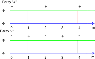
Figure 2: The equivalent wave propagation in ”+” and ”-” ladders. The nodes denote the basis states and the lines the hoppings, the green lines denote $\sqrt{m}(\lambda_{A}+\lambda_{B})$, the blue lines $\sqrt{m}(\lambda_{A}-\lambda_{B})$, the red lines $\omega^{0}_{B}+\omega^{0}_{A}$, the black lines $\omega^{0}_{B}-\omega^{0}_{A}$ and the on-site energies are $\omega m$.

The states are represented by nodes and hoppings between the nodes by the connecting lines. Note that the ladders of Fig. 2 are rather similar to each other, their only difference being the ordering of red and black lines. This becomes very helpful for our calculation given in the Appendix where the computation is shown to simplify in the chosen basis.

The obtained formula for the fidelity can be given in the form

$$\langle\mathcal{F}\rangle=\frac{1}{24}\sum_{m}(Tr[A^{{\dagger}}_{m}A_{m}]+Tr[B^{{\dagger}}_{m}B_{m}]+Tr[C^{{\dagger}}_{m}C_{m}])$$

with

$$A_{m} = f_{m}(+,t)+\sigma^{z}f_{m}(-,t)$$

$$B_{m} = f_{m}(+,t)+(-i\sigma^{y})f_{m}(-,t)\sigma^{x}$$

$$C_{m} = \sigma^{z1}f_{m}(+,t)+\frac{\sigma^{+}}{2}f_{m}(+,t)\sigma^{x}$$

$$+ \frac{\sigma^{-}}{2}f_{m}(-,t)+\sigma^{z2}f_{m}(-,t)\sigma^{x}$$

$$\sigma^{z1} = \left(\begin{array}[]{cc}1&0\\ 0&0\\ \end{array}\right)$$

$$\sigma^{z2} = \left(\begin{array}[]{cc}0&0\\ 0&-1\\ \end{array}\right),$$

where $\sigma^{+,-,z}$ are the Pauli matrices and $f_{m}(\pm,t)$ is the propagator in the ladders shown. In the notation used, e.g. $f_{3}(+,2)$ means the propagator from $m=0$ to slice $m=3$ at time $t=2$ in the ladder with parity ”+”. This gives the fidelity of QST written as a linear combination of the propagators in each of the two ladders.

Since both ladders are semi-infinite the corresponding Hilbert space must be truncated at a maximum phonon number $m$. In order to approximate propagation for very long times long ladders with large maximum $m$ are required. However, a careful study of the formula shows that the fidelity simply arises from the difference between propagators in the two ladders. For example, for $\omega_{A}=0$ or $\omega_{B}=0$ the two ladders are exactly the same and the fidelity becomes precisely zero. Since their structure is rather similar, except for the ordering of lines, if a wave reaches very far from the origin in one of them a very small difference between the two propagators is expected with no contribution to fidelity. Therefore, accurate computations of fidelity do not require very long ladders and reasonable maximum $m$ suffices, as seen in Fig. 3.

Figure 3: The convergence of the average fidelity $\mathcal{F}(t)$ as a function of the maximum phonon number $m$: (a) symmetric case with $\lambda_{A}=\lambda_{B}=1.0$ and $\omega_{A}=\omega_{B}=\omega_{S}$ where the parameters in parentheses on the right of the figure are $(t,\omega_{S})$, and (b) non-symmetric case where the parameters displayed in parentheses are $(\lambda_{A},\lambda_{B},\omega_{A},\omega_{B})$. Time $t$ is set to $32000$.

The accuracy of the computed results is shown in Fig. 3 by plotting the fidelity as a function of the maximum phonon number $m$ for the symmetric case with $\lambda_{A}=\lambda_{B}=\lambda_{S}$, $\omega_{A}=\omega_{B}=\omega_{S}$ and in Fig. 3 for the non-symmetric case. The fidelity is shown to converge very rapidly for maximum phonon numbers $m=40$ or $50$ which permit to use reasonable coupling strengths. The convergence does not depend on time $t_{m}$ and is also rather insensitive to $\omega_{A/B}$ since it mostly depends on the couplings $\lambda_{A/B}$. For example, the numerical results for $\lambda_{S}=1.0$ and $\lambda_{S}=2.0$ required only $m=40$ to $50$ and more that $m=100$, respectively. In our computations suitable maximum $m$ was chosen according to the values of $\lambda_{A/B}$ and the convergence was checked by varying $m$. For couplings $\lambda=0.0$ to $2$ and $\omega=0.0$ to $80$ a maximum phonon number $m$ between $50$ to $110$ was sufficient.

IV Results and Discussion

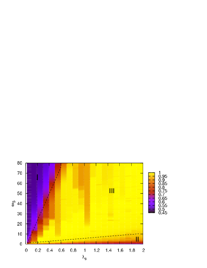
(a) The phase diagram of the maximum fidelity as a function of equal couplings $\lambda_{S}$ and equal qubit separations $\omega_{S}$. Three regions can be distinguished as explained in the text.

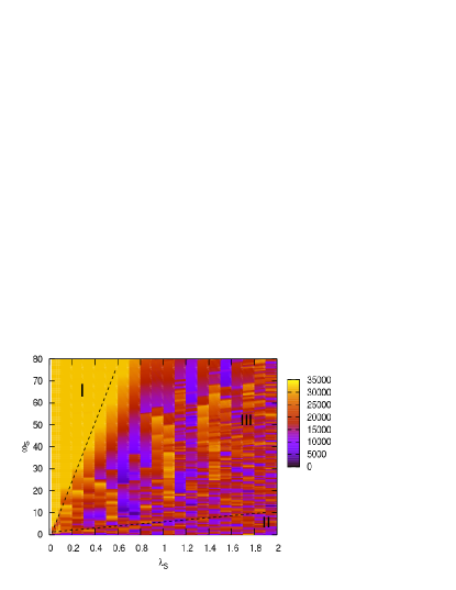
(b) The first peak time of the QST as a function of the equal couplings $\lambda_{S}$ and the qubit separations $\omega_{S}$. This picture also has the three regions mentioned in the text.

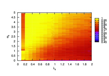
(c) The Region II of Fig.4(a) shown in more detail.

Figure 4: Phase Diagram for the fidelity of QST

The quality of QST is determined by the maximum of the average fidelity $\langle\mathcal{F}\rangle_{m}$ in the time period from $0$ to $t_{m}$ and the time for occurrence of the first peak $t_{p}$ when the system reaches its maximum. Higher fidelity means more faithful state transfer while shorter peak time $t_{p}$ implies faster state transfer. The parameters $\omega_{A}$, $\omega_{B}$, $\lambda_{A}$, $\lambda_{B}$ are taken in units of $\omega=1$ while the maximum fidelity and the first peak time are obtained in the time interval $[0,t_{m}=32\times 10^{3}]$.

IV.1 Phase Diagram for Symmetric Couplings

The phase diagrams of the maximum fidelity and the first peak time are shown in Figs. 4(a), 4(b) as a function of the two parameters $\omega_{S}=\omega_{A}=\omega_{B}$ and $\lambda_{S}=\lambda_{A}=\lambda_{B}$. They can be divided into the following three regions:

Region I: a weak coupling region which lies in the upper left corner of Fig. 4(a) where $\omega_{S}>>\lambda_{S}$. In this case the corresponding first peak time $t_{p}$ shown in Fig. 4(b) is large equal to the upper bound of the chosen time interval $t_{m}$. In other words, the fidelity never reaches its maximum within the adopted evolution time. This indicates that probably a higher fidelity might occur for even longer times so that we can call this a ”slow region”. We may conclude that a good state transfer is impossible in this region because of the long times $t_{p}$.

Region II: lies in the lower part of the figure, which is too small to be seen in Fig. 4(a) and this plot is magnified in Fig. 4(c). In this region $\omega_{S}$ and $\lambda_{S}$ are of the same order of magnitude so that the fidelity is again low but for a different reason than that of region I. The first peak time in this case from Fig. 4(b) is less than $t_{m}$ and the QST is affected by increasing $\omega_{S}$. For zero $\omega_{S}$ no QST is possible while it becomes better when increasing the qubit-environment coupling $\lambda_{S}$.

Region III: The rest of Fig. 4(a). One can see that in the majority of this region high fidelity occurs with the first peak time mostly being less than $5\times 10^{3}$. This region corresponds to a two-valley Hamiltonian and the system behaves as a good quantum channel.

IV.2 Phase diagram for non-Symmetric Couplings

Figure 5: The maximum of the average fidelity $\langle\mathcal{F}\rangle_{m}=0.998$, a value close to a perfect QST, becomes lower for deviations from equal frequencies $\omega_{A}=\omega_{B}=20.0$ and equal couplings $\lambda_{A}=\lambda_{B}=0.8$, with $\delta\omega=\omega_{B}-\omega_{A}$ and $\delta\lambda=\lambda_{B}-\lambda_{A}$, respectively. The $\langle\mathcal{F}\rangle_{m}$ is obtained in the region $[0,33\times 10^{3}]$.

We have also considered the non-symmetric case where the two couplings and the two frequencies are not equal. The influence of a deviation from equal couplings is studied by choosing $\lambda_{S}=0.8,\omega_{S}=20.0$ with the corresponding point of the symmetric phase diagram belonging to region III having very high fidelity equal to $0.998$. A small deviation $\delta\omega$ in $\omega_{B}$ with $\omega_{B}=\omega_{A}+\delta\omega$ is shown in Fig. 5(a) to influence dramatically the QST, which is extremely sensitive even for deviations of the order of $10^{-4}$. The asymmetry in the coupling constants is shown in Fig. 5(b) to have a much smaller effect.

V Conclusions

Although the role of an environment is usually that of causing decoherence for a quantum system the presence of entanglement between the system and the environment also signals the possibility that quantum information can be transferred via the environment. We suggest a QST between two qubits via a coupling to a common boson medium which acts as the quantum channel. We have derived a formula for the corresponding fidelity of the state transfer by mapping this problem into a wave propagation, which is much easier to understand and solve. For symmetric couplings and frequency separation case high fidelity QST between the two qubits is obtained for a wide range of parameters. We show that small deviations from this symmetry can dramatically lower the QST.

Questions for further study are: (i) possible extensions of the present scheme to include a multimode boson environment since our results can cover only approximately the multimode case, (ii) connections of QST to wave propagation in media also in the presence of disorder which can also give ballistic, chaotic and even localized states (in the latter case QST is impossible) and (iii) possible realization of an experiment where QST mediated by bosons can occur, for example, between two quantum dots coupled to the appropriate phonon environment of a nanostructure.

VI Acknowledgment

This work was supported by Marie Curie RTN NANO No 504574 ”Fundamentals in Nanostructures”.

VII Appendix: Derivation of the Formula of Fidelity

The average fidelity

$$\langle\mathcal{F}(t)\rangle=\frac{1}{4\pi}\int d\Omega\langle\psi_{A}|\rho_{B}(t)|\psi_{A}\rangle$$

over $|\psi_{A}\rangle$ becomes

$$|\psi_{A}\rangle = cos(\frac{\theta}{2})|0\rangle+e^{i\phi}sin(\frac{\theta}{2})|1\rangle$$

$$\frac{1}{4\pi}\int d\Omega.. = \frac{1}{4\pi}\int^{\pi}_{0}dsin(\theta)d\theta\int^{2\pi}_{0}d\phi...$$

The reduced density matrix $\rho_{B}(t)$ can be calculated via

$$\rho_{B} = Tr_{A,E}[\rho_{t}]$$

$$\rho_{t} = U(t,0)\rho_{0}U(0,t)$$

$$U(t,0) = e^{iHt}$$

where, the partial trace over the degrees of freedom for qubit A and the quantum channel E is taken. $H$ is the Hamiltonian for the system $A\otimes B\otimes E$ and $U(t,0)$ is the corresponding time evolution operator.

To simplify the formula first we have calculated the integral. It is convenient for us to choose coherent vector representation r6 to express the density matrix.

$$\rho_{B}(t) = \frac{1}{2}(1+\vec{p}_{B}(t)\cdot\vec{\sigma})$$

$$\rho_{A} = \frac{1}{2}(1+\vec{p}_{A}\cdot\vec{\sigma})$$

an assuming the relation between two coherent vectors

$$\vec{p}_{B}(t)=T(t)\cdot\vec{p}_{A}+\vec{T}_{0}(t)$$

we can carry out the integral

$$\langle\mathcal{F}(t)\rangle=\frac{1}{2}[1+\frac{1}{3}Tr(T(t))].$$

We need to calculate the matrix $T(t)$, e.g., to express the final state of qubit B as a function of initial state of qubit A

$$\rho_{B}(t)=Tr_{A,E}[U(t,0)\rho(0)U(0,t)]$$

where $\rho(0)$ is the initial state of the whole system ($A\otimes B\otimes E$), it is separable so that

$$\rho(0) = \rho_{A}(0)\otimes\rho_{B}(0)\otimes\rho_{E}(0)$$

$$\rho_{B}(0) = |0\rangle\langle 0|$$

$$\rho_{E}(0) = |0\rangle\langle 0|.$$

By inserting $|\eta_{A},\eta_{B},m\rangle$ into these formulae we find

$$\rho_{B}(\eta_{B},\eta^{{}^{\prime}}_{B},t)=\sum_{\bar{\eta}_{A},\bar{\eta^{{}^{\prime}}}_{A}}J_{B}(\eta_{B},\eta^{{}^{\prime}}_{B},\bar{\eta}_{A},\bar{\eta^{{}^{\prime}}}_{A},t)\rho_{A}(\bar{\eta}_{A},\bar{\eta^{{}^{\prime}}}_{A},0)$$

$$J_{B}(\eta_{B},\eta^{{}^{\prime}}_{B},\bar{\eta}_{A},\bar{\eta^{{}^{\prime}}}_{A},t) =$$

$$\sum_{\eta_{A}}J(\eta_{A}\eta_{B},\eta_{A}\eta^{{}^{\prime}}_{B},t;\bar{\eta}_{A}0,\bar{\eta^{{}^{\prime}}}_{A}0,0)$$

$$J(\eta_{A}\eta_{B},\eta^{{}^{\prime}}_{A}\eta^{{}^{\prime}}_{B},t;\bar{\eta}_{A}\bar{\eta}_{B},\bar{\eta^{{}^{\prime}}}_{A}\bar{\eta^{{}^{\prime}}}_{B},0) =$$

$$\sum_{m}\langle\bar{\eta}_{A}\bar{\eta}_{B},0|U(0,t)|\eta_{A}\eta_{B},0\rangle\langle\eta^{{}^{\prime}}_{A}\eta^{{}^{\prime}}_{B},0|U(t,0)|\bar{\eta^{{}^{\prime}}}_{A}\bar{\eta^{{}^{\prime}}}_{B},0\rangle,$$

where $\eta_{A/B}=0/1$, $m=0,1,2,3,...$

The matrix element between $\rho_{B}(t)$ and $\rho_{A}(0)$ is related by the function $J_{B}$

$$T=\left(\begin{array}[]{ccc}T^{x}(01)+T^{x}(10)&i[T^{x}(10)-T^{x}(01)]&T^{x}(00)-T^{x}(11)\\ T^{y}(01)+T^{y}(10)&i[T^{y}(10)-T^{y}(01)]&T^{y}(00)-T^{y}(11)\\ T^{z}(01)+T^{z}(10)&i[T^{z}(10)-T^{z}(01)]&T^{z}(00)-T^{z}(11)\end{array}\right)$$

where,

$$T^{x}(\eta\eta^{{}^{\prime}}) = J_{B}(01,\eta\eta^{{}^{\prime}})+J_{B}(10,\eta\eta^{{}^{\prime}})$$

$$T^{y}(\eta\eta^{{}^{\prime}}) = i[J_{B}(10,\eta\eta^{{}^{\prime}})-J_{B}(01,\eta\eta^{{}^{\prime}})]$$

$$T^{z}(\eta\eta^{{}^{\prime}}) = J_{B}(00,\eta\eta^{{}^{\prime}})-J_{B}(11,\eta\eta^{{}^{\prime}})$$

By going into Bell basis the final expression for the fidelity is obtained.

References

- (1) C. H. Bennett, G. Brassard, C. Crpeau, R. Jozsa, A. Peres, and W. K. Wootters, Phys. Rev. Lett. 70, 1895(1993).
- (2) J. I. Cirac, P. Zoller, H. J. Kimble, and H. Mabuchi, Phys. Rev. Lett. 78, 3221 (1997).
- (3) S. Bose, Phys. Rev. Lett. 91, 207901 (2003).
- (4) M. Christandl, N. Datta, A. Ekert, and A. J. Landahl, Phys. Rev. Lett. 92, 187902 (2004).
- (5) Man-Hong Yung, Phys. Rev. A 74, 030303(R) (2006).
- (6) M. Avellino, A. J. Fisher, and S. Bose, Phys. Rev. A 74, 012321 (2006).
- (7) D. Braun, Phys. Rev. Lett. 89, 277901 (2002).
- (8) S.N. Evangelou and A.C. Hewson, J. Phys: Math and Gen.15, 7073-7085 (1982) a numerical renormalisation-group approach for the multi-mode spin-boson model.
- (9) R. Graham and M. Hohnerbach, Consensed Matter 57, 233-248 (1984) for the single mode spin-boson model.
- (10) A. J. Leggett, et al., Rev. Mod. Phys. 59, 1 (1987).
- (11) R. Romano and D. D’Alessandro, Phys. Rev. Lett. 97, 080402 (2006).
- (12) An average fidelity equal to unity means the final state is different from the initial state to be transfered by a phase factor. Since this phase is known via a simple rotation the final state becomes exactly the same as the initial state.