Chaos at the border of criticality

Abstract

The present paper points out to a novel scenario for formation of chaotic attractors in a class of models of excitable cell membranes near an Andronov-Hopf bifurcation (AHB). The mechanism underlying chaotic dynamics admits a simple and visual description in terms of the families of one-dimensional first-return maps, which are constructed using the combination of asymptotic and numerical techniques. The bifurcation structure of the continuous system (specifically, the proximity to a degenerate AHB) endows the Poincare map with distinct qualitative features such as unimodality and the presence of the boundary layer, where the map is strongly expanding. This structure of the map in turn explains the bifurcation scenarios in the continuous system including chaotic mixed-mode oscillations near the border between the regions of sub- and supercritical AHB. The proposed mechanism yields the statistical properties of the mixed-mode oscillations in this regime. The statistics predicted by the analysis of the Poincare map and those observed in the numerical experiments of the continuous system show a very good agreement.

Identifying bifurcation scenarios leading to the formation of chaotic attractors is one of the central problems of nonlinear science. In applications, such information can be used for locating and characterizing the regions of complex behavior. The present paper identifies the proximity to a degenerate Andronov-Hopf bifurcation as a source of complex dynamics in differential equation models of Hodgkin-Huxley type. The latter constitute an important class of models of computational biology. The results of this work explain the origin of chaotic mixed-mode oscillations generated by models of this class and yield the statistical properties of the irregular oscillatory patterns. The statistics predicted by the analysis show a very good agreement with those estimated in the numerical experiments.

1 Introduction

Understanding mechanisms responsible for generating different patterns of electrical activity in neurons, firing patterns, and transitions between them is fundamental for understanding how the nervous system processes information. After a classical series of papers by Alan Hodgkin and Andrew Huxley [10], nonlinear differential equations became a common framework for modeling electrical activity in neural cells. Today the language and techniques of the dynamical systems theory, especially those of the bifurcation theory, are an indispensable part of understanding computational biology. A distinctive feature of many biological models is that they are often close to a bifurcation. In particular, all excitable systems, including many models of neural cells reside near a bifurcation. The type of the bifurcation involved in the mechanism of action potential generation underlies a fundamental classification of neuronal excitability [17]. According to this classification, the excitation in type II models is realized via an AHB. The proximity of a model to an AHB can have a significant impact on the firing patterns that they produce. Near the bifurcation, systems acquire greater flexibility in generating dynamical patterns varying in form and frequency. The proximity to the instability also makes this class of systems more likely to exhibit chaotic behavior. Typical mechanisms of transitions to chaotic dynamics in conductance-based models of neural cells are much less understood compared to those corresponding to periodic activity. Understanding these mechanisms is important in view of the prevalence of irregular dynamics in both modeling and experimental studies of neural cells.

In the present paper, we describe a regime of chaotic mixed-mode oscillations (MMOs) in type II conductance based models. Mixed-mode oscillatory patterns combine small amplitude (subthreshold) oscillations with large amplitude spikes (Fig. 1). Despite subtle underlying dynamical structures, MMOs have been reported in many experimental and modeling studies of neural cells [3, 4, 5, 12, 19, 20] as well as in the models of phenomena outside of neuroscience [6, 15, 22]. The mathematical mechanisms generating MMOs have recently become an area of intense research. Several structures have been proposed to serve as organizing centers for MMOs. Among them, there are folded singularities [1, 14, 23], proximity to the AHB combined with the strongly contracting return mechanism [13], and the Hopf-homoclinic bifurcation [9]. Recent studies have greatly elucidated the sources for periodic mixed-mode regimes. The mechanisms for irregular MMOs remain to be explained. The present paper suggests a general mechanism for chaotic MMOs in terms of the bifurcation structure of the corresponding class of models. Specifically, we show that the transition from supercritical to subcritical AHB in a class of systems lies through the regime of chaotic MMOs. Consequently, systems lying close to such transition are likely to exhibit chaotic behavior. This effect was first noticed in the context of the model of solid fuel combustion in (both in the original infinite dimensional model and its finite dimensional approximation) [6]. The qualitative explanation for the mechanism of chaos near the border of criticality (i.e., where the AHB changes its type from super- to subcritical) for a class of systems, which includes the model in [6] was given in [13]. In the present paper, we show that the necessary ingredients for this scenario are naturally embedded in the structure of type II conductance based models of excitable cells. The latter covers many important biological models, including the Hodgkin-Huxley (HH) model (which we use below to illustrate the proposed mechanism) among many other conductance based models of neurons. We propose a simple geometric mechanism that explains the origins of chaotic dynamics, using a family of one-dimensional ($1D$) unimodal first return maps (Fig. 3). The qualitative features of the Poincare maps such as unimodality and the presence of the boundary layer, where the map is strongly expanding, follow from the proximity of the continuous system to a degenerate AHB and the slow-fast character of the global vector field. Therefore, the bifurcation scenario and the mechanism of chaotic oscillations described below, are independent from the specific details of the model, but are determined by the bifurcation structure pertinent to a whole class of models. Furthermore, we complement and confirm the conclusions of [13] and of this paper on the presence of the chaotic attractors in the corresponding families of models by computing the statistics associated with the irregular MMOs. The latter clearly show that the timings of spikes in the mixed mode patterns are distributed geometrically in accord with our theoretical estimates.

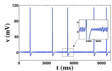
Figure 1: The time series of $v(t)$ of the modified HH model (for the parameter values, see Appendix). In the present regime, the equilibrium of (1), (2) is near the AHB. The bifurcation is subcritical but is very close to the border, where the type of the bifurcation changes to a supercritical. The proximity of the AHB to the border of criticality combined with the slow-fast structure of (1), (2) results in the irregular MMOs shown in this figure.

2 The model

A large class of models of excitable cell membranes relies on the conductance based formalism due to Hodgkin and Huxley [10]. Despite a rich diversity featured by different mathematical models used to elucidate the electrophysiology of various neural cells, many of them share the same structure reminiscent of the classical HH model. Specifically, a typical differential equation model of a (point) neuron consists of a current balance equation and the equations for gating variables, which often present disparate time scales. In identifying new dynamical structures generated by the models of this class, the specific choices of the parameter values in a model at hand may not be so important (unless one is interested in a particular cell type), as they change from one model to another and also depend on many other factors (such as temperature, exposure to neuroactive substances, etc). However, it is critical to preserve the overall structure common to conductance-based models. This is the motivation and the justification for the choice of the model for the present study. The model to be introduced below should not be viewed as a model of a certain neuron, but rather as a representative example of a conductance based model. We consider a modified HH model introduced by Doi and Kumagai [3]. This is a system of nonlinear ordinary differential equations for the membrane potential, $v$, and two gating variables $h$ and $n$:

$$C_{m}\dot{v} = F(v,h,n,I_{ap}),$$ (1)

$$\bar{\tau}_{s}\dot{s} = \frac{s_{\infty}(v)-s}{\tau_{s}(v)},\;s\in\{h,n\},$$ (2)

where $F(v,h,n,I_{ap}):=-g_{Na}m_{\infty}(v)^{3}h(v-E_{Na})-g_{K}n^{4}(v-E_{K})-g_{L}(v-E_{L})+I_{ap}$ is the sum of ionic currents and applied current $I_{ap}$. Constants $E_{c}$ and $g_{c},$ $c\in\left\{Na,K,L\right\}$ stand for reversal potentials and maximal conductances of the corresponding ionic currents. Functions $m_{\infty}(v),s_{\infty}(v)$ and $\tau_{s}(v),$ $s\in\left\{h,n\right\}$ are used in the descriptions of the ionic channels’ kinetics and have typical for the HH model forms. For the analytic expressions of these functions and the values of parameters, we refer the reader to the Appendix to this paper (see also [3]). The only approximation used in the original HH model to obtain (1),(2) is the steady state approximation for gating variable $m\approx m_{\infty}(v)$, which uses the separation of the timescales in the HH model to eliminate the equation for $m$. A mathematical justification of this approximation via a center manifold reduction can be found in [19]. Following [3], we view $\bar{\tau}_{h,n}$ as control parameters, thus, allowing for a range of timescales in (1) and (2). Note that ionic conductances generating electrical activity in different cells have widely varying time constants. Therefore, treating $\bar{\tau}_{h,n}$ as control parameters allows one to investigate the qualitative dynamics for a class of conductance based models, while preserving the biophysical structure of the HH model. In particular, the modified HH model proved very useful for studying mechanisms for MMOs generated by conductance based models [3, 19, 20]. The numerical simulations of the modified HH model [3, 4] revealed multiple parameter configurations producing chaotic MMOs. Below, we describe a general mechanism responsible for generating chaos in this and similar models.

3 The Poincare map

We start by describing the qualitative structure of the model. From (1) and (2) one easily finds the equations for the fixed points:

$$F(\bar{v},h_{\infty}(\bar{v}),n_{\infty}(\bar{v}),I_{ap})=0,\;\bar{s}=s_{\infty}(\bar{v}),\;s\in\{h,n\}.$$ (3)

In the range of parameters of interest, system of equations (1),(2) has a unique fixed point residing near the AHB. In the present study, we fix $\bar{\tau}_{h}=1$ and choose $I_{ap}$ so that the linearization of (1),(2) around $(\bar{v},\bar{h},\bar{n})$ has three eigenvalues:

$$\lambda<0\;\;\mbox{and}\;\;\alpha\pm\beta i,$$ (4)

where $\quad 0<\alpha\ll 1,\beta>0.$ Thus, (1),(2) is close to the AHB. We will use $\bar{\tau}_{n}$ to control the type of the AHB (sub- or supercritical). By a linear change of variables, (1),(2) can be rewritten as

$$\left(\begin{array}[]{c}\dot{\xi}\\ \dot{\eta}_{1}\\ \dot{\eta}_{2}\end{array}\right)=\left(\begin{array}[]{ccc}\lambda&0&0\\ 0&\alpha&-\beta\\ 0&\beta&\alpha\end{array}\right)\left(\begin{array}[]{c}\xi\\ \eta_{1}\\ \eta_{2}\end{array}\right)+{\cal N}(\xi,\eta),$$ (5)

where ${\cal N}$ and $D{\cal N}$ vanish at the origin.

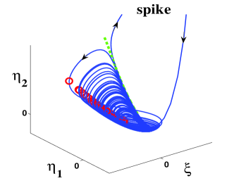
Figure 2: A part of the phase trajectory of (5) is plotted during the phase of the small oscillations between two successive spikes. Prior to leaving a neighborhood of the origin the trajectory remains close to a $2D$ slow manifold. The intersection of the slow manifold with cross-section $\Sigma$ (used for the construction of the Poincare map) is indicated by the line of circles. For computational convenience, in the present study we assumed that $\Sigma$ intersects the slow manifold along the curve of maxima of $\eta_{1}$. Other suitable choices of $\Sigma$ are expected to yield qualitatively similar results.

Near the origin, (5) has a $1D$ local stable manifold $W_{loc}^{s}(O)$ and $2D$ local weakly unstable manifold, $W_{loc}^{u}(O)$.

To describe the mechanism for chaotic oscillations in (5), we refer to the plot of a typical phase trajectory near the origin. The trajectory shown in Fig. 2 approaches a weakly unstable equilibrium at the origin very closely along $W^{s}(O)$ and then spirals out along $W^{u}(O)$. Just near the origin the oscillatory dynamics can be understood via the local analysis of (5) (cf. [13]). The oscillations of the intermediate amplitude shown in Fig. 2 display distinct canard structure. Note that different rings of the spiraling trajectory lie very closely to each other along the dashed curve. The dashed curve in Fig. 2 indicates the canard trajectory separating small and intermediate oscillations from large amplitude spikes [14]. Once the amplitude of oscillations gets sufficiently large, at the end of the long excursion along the dashed curve, the trajectory either escapes from a small neighborhood of the origin and generates a spike, or makes another cycle of oscillations near the origin. The mathematical analysis of canard trajectories in ${\mathbb{R}}^{3}$ and MMOs in general is a difficult and technical problem (see [1, 13, 14, 19, 20, 23]). The irregular MMOs such as shown in Fig. 2 have not been analyzed yet. We will address the mathematical analysis of this problem in the future work. In the present paper, we rely on the numerical observations outlined above, which suggest that near the origin the trajectories remain close to a $2D$ slow manifold. Therefore, the corresponding dynamics can be analyzed with a $1D$ Poincare map. Below, we construct such map using the combination of the analytical and numerical techniques.

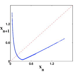
a  b 

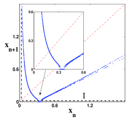
Figure 3: The Poincare maps plotted for two values of the control parameter $\bar{\tau}_{n}:$ $43.02$ (a) and $42.88$ (b). The values of $\bar{\tau}_{n}$ are chosen so that the system is close to the border between the regions of sub- and supercritical AHB. The values of the other parameters are the same as in the Appendix.

To this end, we introduce a cross-section, $\Sigma$, transverse to the slow manifold, and look at the successive intersections of the trajectories of (5) with $\Sigma$ (Fig. 2). The Poincare map has especially convenient form in terms of

$$x=\alpha(\eta_{1}^{2}+\eta_{2}^{2})^{-1}.$$ (6)

Specifically, we define

$$P:x(t_{i})\mapsto x(t_{i+1}),\;i=1,2,...,$$ (7)

where $t_{i}$ are the times of successive crossings of the trajectory of (1), (2) with $\Sigma$. The numerically computed maps for two values of $\bar{\tau}_{n}$ are shown in Fig. 3. Note that the small values of $x$ correspond to the large amplitude oscillations of (5). We are interested in the oscillations of small and intermediate amplitudes. Therefore, in the domain of $P$ we distinguish the region bounded away from some $O(\alpha)$ neighborhood of the origin, $I$, which supports small amplitude oscillations. We call $I$ the principal domain of $P$ (see Fig. 3b). In $I$, $P$ has a distinct layered structure. In the outer region, bounded away from the origin, the map is almost linear. In the complementary boundary layer, the map is unimodal with the slope becoming increasingly steep near the origin (Fig. 3a,b). The almost linear form of the map in the outer region follows from the local analysis of (5) near the origin (cf. [13]):

$$P(x)=x-2\alpha\omega(x+\gamma)+O(\alpha^{2}),\;\omega=2\pi\beta^{-1},$$ (8)

where $\alpha$ and $\beta$ are given in (4). Note that remarkably simple form of the map in (8) is afforded by the choice of the independent variable $x$ (6). The first Lyapunov coefficient $\gamma$ determines the type of the AHB. The bifurcation is subcritical (supercritical) if $\gamma>0(\gamma<0)$. The dynamics of $P$ in the boundary layer corresponds to the canard like oscillations of intermediate amplitude in (5). The formal asymptotic expression for $P$ in the boundary layer can be found in [13]. Providing a rigorous analytical description of $P$ in the boundary layer is beyond the scope of this paper: it requires the information about the canard cycles of (5). For the purposes of the present study, we refer to the numerical results in Fig. 3, which provide a clear evidence in favor of the unimodality of $P$ in the boundary layer. The latter combined with the additive dependence of $P$ on $\gamma$ (see (8)) suggests the mechanism for chaotic MMOs in (5) in the regime $\gamma=O(\alpha)$, i.e. near the border of criticality of the AHB.

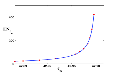
Figure 4: The expected value of the number of small amplitude oscillations, ${\mathbb{E}}N_{\bar{\tau}_{n}}$ as a function of $\tau_{n}$. Numerical data are fitted according to theoretical estimate (9) with $a_{2}\approx 2.34$ and $\bar{\tau}^{1}_{n}\approx 42.983.$

Note that for negative $\gamma=O(1)$, (7) has a unique fixed point, which lies in the outer region (see (8) for the description of $P$ in the outer region). This fixed point corresponds to a stable periodic orbit of (5) born at a supercritical AHB. For increasing values of $\gamma$, by (7), the graph of the map moves down and the fixed point looses stability via a period-doubling bifurcation as it enters the boundary layer (Fig. 3a). This triggers the PD cascade (not shown in this paper; see [13], where it is shown for a closely related model) and leads to the formation of the chaotic attractor in accord with the classical scenario known for unimodal maps [7]. Now we are in a position to describe the mechanism for chaotic MMOs. Note that as long as $\min_{x\in I}P(x)$ remains bounded away from some $O(\alpha)$ neighborhood of $0$ (see Fig. 3a), $P(I)\subset I$ and the dynamics is trapped in $I$. This means that the amplitude of oscillations can not get too big (recall the definition of $x$ in (6)). However, as $\gamma$ is approaching $0$ ($\gamma=O(\alpha)$), the graph of $P(x)$ over $I$ moves down and at some point develops a small window of escape (see the small horizontal segment in the graph of $P$ near the former point of minimum of $P$, Fig. 3b). Now the irregular dynamics in $I$ can be interrupted if the trajectory hits the window of escape. This event, corresponding to a spike in the continuous system (Fig. 1), is followed by the reinjection of the trajectory back to $I$. This in turn initiates a new series of small oscillations. Note that just near the transition from the subthreshold oscillations to MMOs, the size of the window is very small and a typical trajectory stays in $I$ for a long time before escape. Thus, just near the transition point, the typical patterns consist of large (random) number $N_{\bar{\tau}_{n}}$ of small amplitude oscillations between successive spikes. Moreover, assuming that just before the transition, the dynamics in $I$ is mixing, one can show that $N_{\bar{\tau}_{n}}$ is distributed geometrically and estimate the parameter of the geometric distribution (cf. [11]). In the following section, we support the proposed scenario with results of numerical simulations.

4 The statistics of irregular MMOs

In qualitative form, the mechanism generating irregular MMOs in (5) via escape from the principal domain was studied in [11] in the context of chaotic bursting in a class of conductance based models. Note that the differential equation models considered in [11] and in the present paper possess quite different bifurcation structures. The affinity between the mechanisms for chaotic dynamics in these classes of models shows up only after the reduction to suitable $1D$ Poincare maps. While the basis for the reduction to the map is specific to each case, the qualitative properties of the resultant maps are remarkably similar. In particular, the analysis of the statistical properties of the irregular bursting patterns in [11] carries over to that of chaotic MMOs. There are two main outcomes of the analysis in [11]. Translated to the present problem, they can be formulated as follows. Suppose $\bar{\tau}_{n}^{c}$ is a critical value of the control parameter, separating the subthreshold oscillations $(\bar{\tau}_{n}>\bar{\tau}_{n}^{c})$ from the MMOs $(\bar{\tau}_{n}<\bar{\tau}_{n}^{c})$. Suppose, in addition that just before the transition to MMOs the dynamics is mixing. This assumption is motivated by the presence of the steep segment in the graph of the map in the boundary layer near $0$ (see Fig. 3), as well as by the results of direct simulations of (1),(2). Then for $\bar{\tau}_{n}^{c}-\bar{\tau}_{n}>0$ sufficiently small, the number of subthreshold oscillation between successive spikes, $N_{\bar{\tau}_{n}}$, can be approximated by a geometric random variable (cf. [11]). Moreover, by estimating the parameter of the geometric distribution, one can predict the functional form of the dependence of the expected value ${\mathbb{E}}N_{\bar{\tau}_{n}}$ on the distance from the transition point $\bar{\tau}_{n}^{c}-\bar{\tau}_{n}>0$. In particular, the results of [11] imply that near the border of criticality,

$${\mathbb{E}}N_{\bar{\tau}_{n}}\approx\left\{\begin{array}[]{cc}a_{1}\left(\bar{\tau}_{n}-\bar{\tau}^{c}_{n}\right)^{-1/2},&\bar{\tau}_{n}^{1}\lessapprox\bar{\tau}_{n}<\bar{\tau}_{n}^{c},\\ a_{2}\left(\bar{\tau}_{n}-\bar{\tau}^{1}_{n}\right)^{-1},&\bar{\tau}_{n}<\bar{\tau}_{n}^{1},\end{array}\right.$$ (9)

for some positive constants $a_{1},a_{2}$ and for a certain value of $\bar{\tau}_{n}^{1}$, which is less than critical value $\bar{\tau}_{n}^{c}$ but is sufficiently close to it. We verified these prediction numerically for a set of values of $\bar{\tau}_{n}$ near the transition point. In all cases, we found that $N_{\bar{\tau}_{n}}$ are distributed geometrically. A representative plot of the probability density function is shown in Fig. 5. Moreover, the data in Fig. 4 show a very good fit with the theoretical estimate in the second line of (9). We did not attempt numerical verification of the estimate in the top line of (9), because it requires numerical integration of (1),(2) over extremely long intervals of time and is expected to hold in a rather narrow interval of $\bar{\tau}_{n}$. In addition to verifying (9), the numerical experiments presented in this section support the claim that the dynamics of (1),(2) near the border of criticality is chaotic. In particular, the fact that the distribution of $N_{\bar{\tau}_{n}}$ is geometric provides a posteriori justification for the assumption that dynamics of $P$ is mixing in $I$, which was used in [11] to infer that $N_{\bar{\tau}_{n}}$ is approximately a geometric random variable and to derive (9). Therefore, the map-based description of the transformations in the dynamics of (1) and (2), which accompany the approach of the border between regions of supercritical and subcritical AHB, combined with the numerical results presented in this section form a convincing evidence of the existence of the chaotic attractor in this regime. We emphasize the universal character of this effect: the principal ingredients necessary for its realization such as the proximity to a degenerate AHB and the reinjection mechanism are expected to be present in a large class of systems. In particular, the same mechanism is responsible for generating chaotic MMOs in a model of solid fuel combustion [13]. The results of the present study suggest that it is relevant for an important class of biological models.

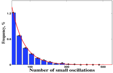
Figure 5: The probability distribution of the number of oscillations between two successive spikes in a typical trajectory of (1),(2) for $\bar{\tau}_{n}\approx 42.95.$ The histogram for $N_{\tau_{n}}$ is obtained using the numerical data for $10^{3}$ interspike intervals and is fitted with the exponential probability density function approximating a shifted geometric distribution: $7+\mbox{Geom(66.5)}$ (plotted with solid line).

5 Discussion

Substantial efforts have been made to identify and to understand the mechanisms generating chaotic dynamics in physical and biological systems, and in particular, in conductance based models of neural cells [2, 8, 11, 16, 21]. In the context of neuronal modeling, understanding the sources of chaos is important for elucidating the origins and characterizing the properties of patterns of irregular electrical activity in the nervous system. The latter are quite common on both cellular and network levels. There is a compelling evidence showing that irregular firing in many cases results from the intrinsic properties of neural cells and their networks, rather than from random fluctuations. Although, there is no complete understanding for the functional role of chaos in neural systems, there are several lines of evidence indicating its potential importance. First, there are modeling studies suggesting that chaotic elements enhance the information processing properties of the networks that they form [16]. Second, the loss of regularity in certain patterns of neural activity are known to accompany the onset of some pathological states, such as epileptic seizures and Parkinsonian states. Therefore, better understanding of the origins of chaos in neuronal models may help to predict the onset of pathological states and to control them. Single cell models such as (1),(2) provide the simplest biophysically meaningful framework for studying chaos in neuronal dynamics. Our study supports the view that chaotic dynamics is a likely attribute of a system operating on the edge of instability [16]. Note that on the border of criticality, the regime of interest in our study, type II models acquire remarkable pattern-forming capacity and flexibility: upon relatively small changes of parameters they exhibit a rich repertoire of qualitatively different patterns ranging from subthreshold oscillations (supercritical AHB) to a variety of periodic and aperiodic MMOs (subcritical AHB) [3, 13]. Thus, the ability of the system to detect and to encode small changes in the stimulus is greatly enhanced in this regime. The present paper points out that in a broad class of type II models of neural cells, the proximity to the border of criticality of the underlying AHB, implies chaotic dynamics. Moreover, the results in [13] suggest that under certain natural constraints, for small $\alpha>0$, this is the only region in the parameter space of (1), (2), where robust chaotic oscillations are expected. For this regime, we provide a geometric explanation for the mechanism of chaotic dynamics, using a family of $1D$ Poincare maps. We conducted a series of numerical experiments to verify our theoretical predictions and found that the former are in a good agreement with the latter. Our results can be used to locate chaotic regimes in type II models and to describe the statistical properties of the resultant oscillatory patterns. Finally, we emphasize that the results of the present study apply to a class of conductance based models (for which (1),(2) is only a representative example), as well as to models outside biology. In particular, we have obtained qualitatively similar results (including the statistical data as shown in Fig. 4 and 5) for a model of solid fuel combustion [6, 13]. The type of the AHB in many conductance-base models (including the original HH model) can be switched from sub- to supercritical by varying parameters in physiologically relevant ranges [18]. Therefore, the results of this paper are relevant to explaining firing patterns generated by this class of models.

Acknowledgments. One of the authors (GM) would like to thank Victor Roytburd for useful conversations. This work was partially supported by the National Science Foundation under Grant No. 0417624.

Appendix. Parameter values.

In this appendix, we list the expressions of various functions, which appear on the right hand sides of (1) and (2):

$$\tau_{s}(v)={1\over\alpha_{s}(v)+\beta_{s}(v)},\;s\in\{h,n\}, c_{\infty}(v)={\alpha_{c}(v)\over\alpha_{c}(v)+\beta_{c}(v)},\;c\in\{m,n,h\},$$

$$\alpha_{m}(v)={0.1(25-v)\over\exp\{{25-v\over 10}\}-1}, \beta_{m}(v)=4\exp\{{-v\over 18}\}$$

$$\alpha_{n}(v)={0.01(10-v)\over\exp\{{10-v\over 10}\}-1}, \beta_{n}(v)=0.125\exp\{{-v\over 80}\}$$

$$\alpha_{h}(v)=0.07\exp\left\{{-(v-8)\over 20}\right\}, \beta_{h}(v)={1\over\exp\{{38-v\over 10}\}+1}$$

Here, $v$, the membrane potential, is in mV. The gating variables $n$ and $h$ are nondimensional. The values and the units of the parameter values in (1) and (2), which were used to generate Fig. 1-5 are given in the following table:

$I_{ap}$	$0.6\;\mu\mbox{A/cm}^{2}$	$\bar{\tau}_{h}$	$1$	$\bar{g}_{Na}$	$120\;\mbox{mS/cm}^{2}$	$\bar{g}_{K}$	$36\;\mbox{mS/cm}^{2}$
$\bar{g}_{L}$	$0.3\;\mbox{mS/cm}^{2}$	$E_{Na}$	$115\;\mbox{mV}$	$E_{K}$	$-12\;\mbox{mV}$	$E_{L}$	$10.599\;\mbox{mV}$

The time constant $\bar{\tau}_{n}$ is viewed as a control parameter. We used $\bar{\tau}_{n}=42.925$ to generate Fig. 1 and Fig. 2. For the values of $\bar{\tau}_{n}$ used for other plots, we refer the reader to the captions of the corresponding figures.

References

- [1] M. Brns, M. Krupa, and M. Wechselberger, Mixed-mode oscillations due to generalized canard phenomenon, Fields Inst. Comm., , 39–64, 2006.
- [2] T.R. Chay and J. Rinzel, Bursting, beating, and chaos in an excitable membrane model, Biophys. J., , 357–366, 1985.
- [3] S. Doi and S. Kumagai, Generation of very slow neuronal rhythms and chaos near the Hopf bifurcation in single neuron models, J. Comp. Neurosc., , 325–356, 2005.
- [4] S. Doi, S. Nabetani, and S. Kumagai, Complex nonlinear dynamics of the Hodgkin-Huxley equations induced by time scale changes, Biological Cybernetics, , 51–64, 2001.
- [5] J. Drover, J. Rubin, J. Su, and B. Ermentrout, Analysis of a canard mechanism by which excitatory synaptic coupling can synchronize neurons at low firing frequencies, SIAM J. Appl. Math., , 69–92, 2004.
- [6] M. Frankel, G. Kovacic, V. Roytburd, and I. Timofeyev, Finite-dimensional dynamical system modeling thermal instabilities, Physica D, , 295–315, 2000.
- [7] J. Guckenheimer and P. Holmes, Nonlinear Oscillations, Dynamical Systems, and Bifurcations of Vector Fields, Springer, 1983.
- [8] J. Guckenheimer and R.A. Oliva, Chaos in the Hodgkin–Huxley Model, SIAM J. Appl. Dyn. Syst., 1 (1), 105–114, 2002.
- [9] J. Guckenheimer and A.R. Willms, Asymptotic analysis of subcritical Hopf-homoclinic bifurcation, Physica D, , 195–216, 2000.
- [10] A.L. Hodgkin and A.F. Huxley, A quantitative description of membrane current and its application to conduction and excitation in nerve, J. Physiol., , 500–544, 1952.
- [11] G. Medvedev, Transition to bursting via deterministic chaos, Phys. Rev. Lett., , 048102 (2006).
- [12] G. Medvedev and J.E. Cisternas, Multimodal regimes in a compartmental model of the dopamine neuron, Physica D, (3-4), 333-356, 2004.
- [13] G. Medvedev and Y. Yoo, Multimodal oscillations in systems with strong contraction, Physica D, , 87–106, 2007.
- [14] A. Milik and P. Szmolyan, Multiple time scales and canards in a chemical oscillator, in C.K.R.T. Jones and A. Khibnik, eds, Multiple-Time-Scale Dynamical Systems, Springer, 2000.
- [15] A. Milik, P. Szmolyan, H. Lffelman, and E. Grller, Geometry of mixed-mode oscillations in the 3-D autocatalator, Intern. J. of Bifurc. and Chaos, , 505–519, 1998.
- [16] M.I. Rabinovich, P. Varona, A.I. Selverston, H.D.I. Abarbanel, Dynamical Principles in Neuroscience, Reviews of Modern Physics, 1213, 2006.
- [17] J. Rinzel and G.B. Ermentrout, Analysis of neural excitability and oscillations, in C. Koch and I. Segev, eds Methods in Neuronal Modeling, MIT Press, Cambridge, MA, 1989.
- [18] J. Rinzel and R.N. Miller, Numerical computation of stable and unstable periodic orbits in the Hodgkin-Huxley equations, Math. Biosci., , 27-59, 1980.
- [19] J. Rubin and M. Wechselberger, Giant squid - hidden canard: the 3D geometry of the Hodgkin-Huxley model”, Biological Cybernetics, , 5–32, 2007.
- [20] J. Rubin and M. Wechselberger, The selection of mixed-mode oscillations in a Hodgkin-Huxley model with multiple time scales, CHAOS, , 015105, 2008.
- [21] D. Terman, Chaotic spikes arising from a model of bursting in excitable membranes, SIAM J. Appl. Math., , 1418–1450, 1991.
- [22] E.I. Volkov and D.V. Volkov, Multirhythmicity generated by slow variable diffusion in a ring of relaxation oscillators and noise-induced abnormal interspike variability, Phys. Rew. E, , 2002.
- [23] M. Wechselberger, Existence and Bifurcation of Canards in in the case of a Folded Node, SIAM J. Applied Dynamical Systems, (1), 101-139, 2005.