The Evolution of the Cosmic Microwave Background

Abstract

We discuss the time dependence and future of the Cosmic Microwave Background (CMB) in the context of the standard cosmological model, in which we are now entering a state of endless accelerated expansion. The mean temperature will simply decrease until it reaches the effective temperature of the de Sitter vacuum, while the dipole will oscillate as the Sun orbits the Galaxy. However, the higher CMB multipoles have a richer phenomenology. The CMB anisotropy power spectrum will for the most part simply project to smaller scales, as the comoving distance to last scattering increases, and we derive a scaling relation that describes this behaviour. However, there will also be a dramatic increase in the integrated Sachs-Wolfe contribution at low multipoles. We also discuss the effects of tensor modes and optical depth due to Thomson scattering. We introduce a correlation function relating the sky maps at two times and the closely related power spectrum of the difference map. We compute the evolution both analytically and numerically, and present simulated future sky maps.

I Introduction

The Cosmic Microwave Background (CMB) radiation provides us with a vital link to the epoch before the formation of distinct structures, when fluctuations were still linear and carried in a very clean way information about their origin, presumably during a phase of inflation. The simple dynamics of the generation and propagation of CMB anisotropies (see e.g. Refs. Scott and Smoot (2006); Challinor (2004); Hu and Dodelson (2002) and references therein) depends on a handful of cosmological parameters, $P_{i}$, such as the Hubble constant, the matter density, and spatial curvature, in addition to the initial conditions set through inflation. These dependencies have been thoroughly investigated over the past couple of decades and form the basis for estimating the parameters from the observed anisotropy spectrum of the CMB.

However, there is one dimension in the parameter space of the CMB that has received little explicit attention. For fixed matter content and curvature of the Universe today, we still have the freedom to evolve the CMB anisotropies forwards or backwards in time. For the practical business of performing CMB parameter estimation, it is natural of course to suppress this freedom, since we are interested in predicting the anisotropies today. The constraint to “today” can be applied in at least two ways, which it is important to distinguish. From the set of parameters $P_{i}$ we can calculate the proper-time age of the Universe, $t_{0}$. This quantity is only determined to an accuracy set by the parameters $P_{i}$ (e.g. using Wilkinson Microwave Anisotropy Probe (WMAP) 3-year data, Spergel et al. Spergel et al. (2007) find that $t_{0}=13.73^{+0.13}_{-0.17}$ Gyr). However, the WMAP results constrain the redshift of last scattering, $z_{\rm rec}$, (defined as the centre of the recombination epoch) to much greater accuracy: $z_{\rm rec}=1088^{+1}_{-2}$ Spergel et al. (2003). This very small uncertainty is the result of our accurate determination of the mean temperature of the CMB, $T=2.725\,\pm\,0.001$ K Fixsen et al. (1996); Mather et al. (1999). Thus, even though $t_{0}$ is only known to an accuracy comparable to the other parameters $P_{i}$, implicit in analyses of the CMB is the very tight constraint on a different temporal coordinate, $z_{\rm rec}$ or $T$.

Essentially, the constraint on $t_{0}$ arises from our determination of the expansion rate today, together with information on the content and geometry of the Universe, which affect its expansion history. The constraint on $T$ is entirely independent of the content or geometry, hence its superior accuracy. Popular CMB anisotropy numerical packages, such as cmbfast or camb Lewis et al. (2000); Seljak and Zaldarriaga (1996) impose the tight constraint arising from the mean temperature through an input parameter. This constraint on $T$ is equivalent, via the Stefan-Boltzmann law, to a constraint on the energy density in CMB radiation, $\rho_{\gamma}$. Therefore by adjusting the temperature input parameter, and other cosmological input parameters accordingly, it is possible to generate spectra with these packages that correspond to a given model evolved into the past or future. Alternatively it is possible to modify the code in these packages to directly integrate to future times without the need to modify the input parameters. Note that if we just vary the proper age $t_{0}$ of a model by varying the expansion rate today, this necessarily changes the relative contributions of matter and radiation in the past, which affects the physics at recombination and hence the shape of the CMB spectrum.

Fortunately the required code modifications are relatively straightforward, and in addition it is possible to describe the temporal evolution of the CMB anisotropies analytically to very high precision. In this work we systematically describe this evolution both numerically and analytically, within the context of the standard $\Lambda$CDM ($\Lambda$ Cold Dark Matter) model, in order to complete the standard results on the parametric dependence of the CMB. The verification of our numerical work with our analytical results, and conversely the characterization of our analytical approximations with the full numerical calculations, will be crucial in this novel study. We will find that while the temporal behaviour of the CMB power spectrum is determined mainly by a simple geometrical scaling relationship, less trivial physics arises when we consider the behaviour of correlations between anisotropies at different times.

It can certainly be argued that the standard calculations of the CMB anisotropy spectrum implicity describe its time dependence in that the spectrum must be evolved from the time of recombination to the present. Nevertheless, there appear to have been very few explicit discussions of the time dependence, with the exceptions being primarily concerned with the distant future. Gott Gott (1996) points out that at extremely late times the typical wavelengths of CMB radiation will exceed the Hubble radius, and so the CMB radiation will be lost in a de Sitter background. Loeb Loeb (2002) mentions that as the time of observation increases, the radius of the last scattering sphere also increases, and approaches a maximum in a $\Lambda$CDM model. This leads to the potential for reducing the cosmic variance limitation on the determination of the anisotropy spectrum. Krauss and Scherrer Krauss and Scherrer (2007) point out that well before this final stage, the CMB will redshift below the plasma frequency of the interstellar medium and hence be screened from view inside galaxies.

Importantly, when discussing the distant future evolution of the Universe it must be remembered that even the qualitative details can depend very sensitively on the model adopted. An extreme example is the potential destruction of the Universe in finite proper time in a “big rip” Caldwell et al. (2003), when the dark energy violates the weak energy condition, with equation of state $w<-1$. In the present work, for the sake of definiteness and simplicity, we conservatively choose a spatially flat model in which the dark energy is a pure cosmological constant, with cosmological parameters consistent with the WMAP results Spergel et al. (2007). However, using the techniques we discuss it is straightforward to extend our results to other specific dark energy models.

An interesting question that naturally arises in the present context is: How long must we wait before we could observe a change in the CMB? The formalism that we develop here will be necessary to answer this question, and we will address this explicit issue in separate work Moss et al. (2007). We stress that the practicalities of an experimental search for the effects we describe is not our concern in the present work. In addition to setting the stage for the detectability question, we believe that a discussion of the evolution of the CMB sky is useful in its own right in elucidating the physics of the anisotropies in a vacuum-dominated cosmology.

We begin in Section II with a description of the time dependence of the “bulk” properties of the CMB, namely the mean temperature and the dipole. After a brief review of the formalism used to describe the anisotropy power spectrum, its evolution is described analytically in Section III, including the effects of the integrated Sachs-Wolfe effect, tensor modes, and reionization, and numerical calculations are presented using our modified version of the line-of-sight Boltzmann code camb. In Section IV we introduce the difference map power spectrum and associated correlation function, and present analytical and numerical calculations. Section V presents our conclusions, and in the Appendix a description of an important approximation method is presented. We set $c=1$ throughout.

II Time evolution of the bulk CMB

The temperature fluctuations on the CMB sky can be decomposed into a set of amplitudes of spherical harmonics (see Section III.1). The angular mean temperature (or “monopole”) and dipole have a special status. The mean temperature is just a measure of the local radiation energy density, while the value of the dipole depends on the observer’s reference frame at linear order (higher multipoles are independent of frame at this order).

II.1 The mean temperature

As time passes, the change in the CMB that is simplest to quantify is the cooling of its mean temperature $T$ due to the Universe’s expansion. The CMB radiation was released from the matter at the time of last scattering, when $T\simeq 3000$ K. It later reached a comfortable $300$ K at an age of about $t\simeq 15$ Myr, and is now only a frigid few Kelvin. Indeed, the monotonicity of the function $T(t)$ means that $T$ itself can be used as a good time variable. Thus we can consider measurements of $T$ as direct readings of a sort of “cosmic clock”.

Today the CMB radiation is essentially free streaming, i.e. non-interacting with the other components of the Universe. Therefore the energy density in the CMB evolves according to the energy conservation equation $\dot{\rho}_{\gamma}=-4H\rho_{\gamma}$, where $H$ is the Hubble parameter and the overdot represents the proper time derivative. Since $\rho_{\gamma}\propto T^{4}$, we have $\dot{T}=-HT$. Evaluating this expression today, using $T_{0}=2.725$ K and $H_{0}=73$ km s${}^{-1}\,$Mpc^-1 (subscript ₀ indicates values today), we find

$$\dot{T}_{0}=-0.20\ \mu\mathrm{K}\ \mathrm{kyr}^{-1}.$$ (1)

Thus in $5000$ yr the mean temperature will drop by $1\ \mu$K.

The CMB radiation continues to redshift indefinitely as the Universe expands in the late $\Lambda$-dominated de Sitter phase. However, this does not mean that as the CMB becomes increasingly difficult to measure, clever experimentalists need only to ever refine their instruments in order to keep up. Instead, a fundamental limit exists below which a CMB temperature cannot be sensibly defined. An object in an otherwise empty de Sitter phase will see a thermal field with temperature Gibbons and Hawking (1977)

$$T_{\rm dS}=\frac{H}{2\pi}=\frac{1}{2\pi}\sqrt{\frac{\Lambda}{3}}.$$ (2)

Therefore, after the CMB temperature redshifts to below $T_{\rm dS}$, the CMB becomes lost in the thermal noise of the de Sitter background, as pointed out in Gott (1996) (see also Busha et al. (2003)).

To see explicitly the difficulty with measuring the CMB at such extremely late times, consider the typical wavelengths of radiation in the CMB. A thermal spectrum at temperature $T$ consists of wavelengths $\lambda$ on the characteristic scale $T^{-1}$ (the precise peak position of the Planck spectrum depends on the measure used for the thermal distribution). Therefore when $T=T_{\rm dS}$ we have $\lambda\simeq H^{-1}$, i.e. the typical CMB wavelengths become of order the Hubble length. Alternatively, at late times in the de Sitter phase the frequency of a mode of CMB radiation of fixed comoving wavelength redshifts according to

$$\omega(t)=\omega(t_{1})e^{-H_{\rm dS}(t-t_{1})},$$ (3)

where

$$H_{\rm dS}\equiv\sqrt{\Omega_{\Lambda}}H_{0}$$ (4)

is the asymptotic value of the Hubble parameter and $t_{1}$ is some late proper time. Therefore the accumulated phase shift between time $t_{1}$ and the infinite future is

$$\int_{t_{1}}^{\infty}\omega(t)dt=\frac{\omega(t_{1})}{H_{\rm dS}}.$$ (5)

This expression tells us that when the frequency becomes less than the Hubble parameter (i.e. the wavelength becomes larger than the Hubble length), a full temporal oscillation cannot be observed, even if we observe into the infinite future. In terms of conformal time, the oscillation rate remains constant in the de Sitter phase, but there is only a finite amount of conformal time available in the future. Indeed, considering the quantum nature of such a mode, this calculation provides insight into the necessity of a residual de Sitter thermal spectrum at this scale.

The energy density in the CMB at arbitrary scale factor $a$ is given by

$$\rho_{\gamma}=\frac{3H_{0}^{2}m_{\rm P}^{2}\Omega_{\gamma}}{8\pi}\left(\frac{a_{0}}{a}\right)^{4},$$ (6)

where $m_{\rm P}$ is the Planck mass and $\Omega_{\gamma}=5\times 10^{-5}$ is the fraction of the total density in the CMB today. Using this expression we can show that we must wait until $a/a_{0}\sim 10^{30}$ before $\rho_{\gamma}=\rho_{\rm dS}\equiv T_{\rm dS}^{4}$ and the CMB becomes lost in the de Sitter background. This corresponds to an age of $t=1$ Tyr. If we ask instead at what scale factor would the radiation density be equal to the Planck density, $\rho_{\rm P}=m_{\rm P}^{4}$, we find $a/a_{0}\sim 10^{-32}$. It might appear, therefore, that we exist at a special time, in that the radiation density today is roughly $120$ decades removed from both the Planck era and the final era when $T=T_{\rm dS}$. To understand the origin of this coincidence, note that by virtue of the above expressions and the energy constraint (or Friedmann) equation, the three densities $\rho_{\rm P}$, $\rho_{\Lambda}$, and $\rho_{\rm dS}$ are in the geometrical ratio $m_{\rm P}^{4}:\Lambda m_{\rm P}^{2}:\Lambda^{2}$, up to numerical factors. Therefore, the apparent coincidence just described is actually equivalent to the standard coincidence problem, namely that $\rho_{\Lambda}\simeq\rho_{\rm tot}$ today, given that $\rho_{\gamma}$ differs from $\rho_{\rm tot}$ today by “only” a few decades. Any density that today even crudely approximates the dark energy density will necessarily be separated by roughly $120$ decades from both $\rho_{\rm P}$ and $\rho_{\rm dS}$.

II.2 The dipole

The observed dipole anisotropy in the CMB can be attributed to the Doppler effect arising from our peculiar velocity, $\boldsymbol{v}$, with respect to the frame in which the CMB dipole vanishes. That peculiar velocity, and hence the dipole, is expected to evolve with time. The magnitude of the dipole can be specified by the maximum CMB temperature shift over the sky, $\delta T_{d}$, due to the velocity $\boldsymbol{v}$. This is given by the lowest order Doppler expression,

$$\frac{\delta T_{d}}{T}=v.$$ (7)

(In terms of the spherical harmonic expansion to be introduced in Eq. (15), we have $\delta T_{d}/T=\sqrt{3/(4\pi)}a_{10}$, when the polar axis is aligned with $\boldsymbol{v}$.)

The current best estimate of the magnitude of the dipole comes from observations of the WMAP satellite—indeed, the annual modulation by the Earth’s motion around the Sun is actually used to calibrate satellite experiments, so this aspect of the time-varying dipole is already well determined. The measured value of the dipole, in Galactic polar coordinates, is $(\delta T_{d},l,b)=(3.358\pm 0.0017$ mK, $263.86\pm 0.04^{\circ}$, $48.24\pm 0.10^{\circ})$ Hinshaw et al. (2007). Equivalently, the Cartesian velocity vector is $\boldsymbol{v}_{0}\simeq(-26.3$, $-244.6$, $275.6)$ km$\,{\rm s}^{-1}$, where the first component is towards the Galactic centre, and the third component is normal to the Galactic plane. Therefore, in natural units we have $v_{0}=1.2\times 10^{-3}$, so the lowest order approximation, Eq. (7), is valid.

In order to determine the evolution of the dipole, we could straightforwardly calculate it at linear order. However, linear theory is certainly not a good approximation on sufficiently small scales today. To fully describe the evolution of the velocity $\boldsymbol{v}$ we must take into account the presence of the nonlinear structures we observe on small scales today.

This velocity vector can be considered as a sum of individual vectors contributing to the overall motion of the Sun with respect to the CMB. In the local neighbourhood, the Sun moves with respect to the “local standard of rest”, which in turn moves with respect to the Galactic centre. However, the peculiar motions in the Solar neighbourhood are at the 10% level compared with the motion of the Sun around the Milky Way Kogut et al. (1993), so for the purposes of the simple calculation which follows we ignore these contributions. Also, we will consider here time scales short enough that the motion of the Milky Way within the Local Group, and the Local Group relative to Virgo, the Great Attractor, and other distant cosmic structures is approximately constant (see, e.g., Tully et al. (2007) for a description of these motions).

Just as today we can detect the modulation of the Earth’s motion around the Sun, in the future, with increasing satellite sensitivity, we may be able to observe the Sun’s motion around the Galaxy. For the motion of the Sun around the Milky Way, we assume that this is simply a tangential speed of $220$ km$\,{\rm s}^{-1}$ at a distance of $8.5$ kpc. Using the current observed value of $\boldsymbol{v}$ to infer the velocity of the Galactic centre with respect to the CMB rest frame, the time dependent Sun-CMB velocity vector is then

$$\boldsymbol{v}(t)=\bigg{[}\!\!\! 222\sin\left(\frac{2\pi t}{T}\right)-26.3,$$ (8)

$$222\cos\left(\frac{2\pi t}{T}\right)-466.6,\>275.6\bigg{]}{\rm km}\,{\rm s}^{-1}\,,$$

where the Galactic orbital period is $T=2.35\times 10^{8}$ yr.

In order to ascertain when a change in the dipole is detectable, one could compute a sky map of the dipole at two times. If the temperature variance of the difference map is greater than the experimental noise variance, then a detection is probable. In this case, the variance of the difference map, which we denote by $C_{S}$, is $C_{S}=[(\delta v_{x})^{2}+(\delta v_{y})^{2}+(\delta v_{z})^{2}]/(4\pi)$, where $\delta\boldsymbol{v}$ is the difference of the Sun-CMB dipole vector between the two observations. Using Eq. (8), and converting to fractional temperature variations, the signal variance of the changing dipole is then

$$C_{S}=8.7\times 10^{-8}\left[1-\cos\left(\frac{2\pi t}{T}\right)\right]\,.$$ (9)

Later in this paper we compute signal variances involving higher order CMB multipoles. These variances are of course much smaller than that of the dipole. In a follow up paper Moss et al. (2007) we will discuss in detail the prospects for detecting a change in the CMB with future experiments.

Finally, we note that in this simple calculation it is assumed that we have a frame of reference external to the Milky Way in order to construct our coordinate system. This could be provided, for example, by the International Celestial Reference Frame, based on the positions of 212 extra-galactic sources Ma et al. (1998).

III The anisotropy power spectrum

III.1 Review of the basic formalism

There is much more information encoded in the anisotropies of the CMB than in the mean temperature, since the anisotropies are determined by the details of the matter and metric fluctuations near the last-scattering surface (LSS) and all along our past light cone to today. Therefore it is much less trivial to determine the time evolution of the anisotropies than the mean temperature (or dipole). However, in the approximation that all of the CMB radiation was emitted from the LSS at some instant $t_{\rm LS}$ when electrons and photons decoupled, and then propagated freely, the evolution of the primary power spectrum of the CMB is determined by a simple geometrical scaling relation which is closely related to the main geometrical parameter degeneracy in CMB spectra. In order to derive this relation, and to describe the behaviour of the correlation functions introduced in later sections, it will be helpful to first summarize the standard description of CMB anisotropies in a form that will be easy to generalize. This subsection may be skipped by readers familiar with the material. For detailed treatments of the generation of anisotropies see e.g. Hu and Sugiyama (1995); Dodelson (2003).

At very early times, when each perturbation mode, labelled by comoving wavevector ${\boldsymbol{k}}$, is outside of the Hubble radius, the fluctuations can be described by a single perturbation function, for the case of adiabatic perturbations. It is very convenient to take this function to be the curvature perturbation on comoving hypersurfaces, ${\cal R}$, since this quantity is conserved on large scales in this case, and hence can be readily tied to the predictions of a specific inflationary model. In the simplest models of inflation, ${\cal R}$ is predicted to be a Gaussian random field to very good approximation, fully described by the relation

$$\langle{\cal R}^{\ast}({\boldsymbol{k}}){\cal R}({\boldsymbol{k}}^{\prime})\rangle=2\pi^{2}\delta^{3}({\boldsymbol{k}}-{\boldsymbol{k}}^{\prime})\frac{{\cal P_{\cal R}}(k)}{k^{3}},$$ (10)

with primordial power spectrum ${\cal P_{\cal R}}(k)$ and $k\equiv|{\boldsymbol{k}}|$. For a scale-invariant spectrum we have ${\cal P_{\cal R}}(k)=$ constant.

The fluctuations at last scattering can be described by a set of matter and metric perturbations, $\phi_{i}({\boldsymbol{x}},\eta)$, where for future convenience we have used comoving coordinate ${\boldsymbol{x}}$ and conformal time $\eta$. Since linear perturbation theory is a very good approximation at the scales sampled by the CMB, this set of perturbations is determined from the primordial comoving curvature perturbation by transfer functions $A_{i}(k,\eta)$ via

$$\phi_{i}({\boldsymbol{k}},\eta)=A_{i}(k,\eta){\cal R}({\boldsymbol{k}}).$$ (11)

In the approximation of abrupt recombination, so that the LSS has zero thickness, followed by free streaming of radiation, the observed primary temperature anisotropy $\delta T(\boldsymbol{\hat{e}})/T$ in direction $\boldsymbol{\hat{e}}$ is determined by the fluctuations at the corresponding point on the LSS, i.e.

$$\frac{\delta T(\boldsymbol{\hat{e}},\eta)}{T(\eta)}=F(\phi_{i}(r_{\rm LS},\boldsymbol{\hat{e}},\eta_{\rm LS})),$$ (12)

for some linear function $F$. Here $r_{\rm LS}=\eta-\eta_{\rm LS}$ is the comoving radial coordinate to the LSS from the point of observation, taken to be the origin of spherical coordinates. Eq. (12) ignores both the effect of gravitational lensing by foreground structure and the effect of reionization at late times (we examine the effects of reionization in Section III.5). In the approximation that photons are tightly coupled to baryons before $\eta_{\rm LS}$, the function $F$ can be written in terms of two perturbation functions as

$$F(\phi_{i}(r_{\rm LS},\boldsymbol{\hat{e}},\eta_{\rm LS}))=\phi_{1}(r_{\rm LS},\boldsymbol{\hat{e}},\eta_{\rm LS})+\frac{\partial}{\partial r_{\rm LS}}\phi_{2}(r_{\rm LS},\boldsymbol{\hat{e}},\eta_{\rm LS}).$$ (13)

Eqs. (12) and (13) describe the generation of CMB anisotropies through the Sachs-Wolfe effect Sachs and Wolfe (1967), with the first term on the right-hand side of (13) the so-called “monopole” contribution, and the second term the “dipole” or “Doppler” contribution.

The preceeding equations have the very simple interpretation that when we measure the CMB anisotropies at some time $\eta$ we are “seeing” the primordial fluctuations ${\cal R}$ on the comoving spherical shell $r=r_{\rm LS}=\eta-\eta_{\rm LS}$, as processed by the linear transfer functions $A_{1}$ and $A_{2}$ to the time $\eta_{\rm LS}$. If we observe at a later time $\eta^{\prime}$, we see the fluctuations on a larger shell of radius $r=r_{\rm LS}^{\prime}\equiv\eta^{\prime}-\eta_{\rm LS}$, as illustrated in Fig. 1. The fluctuations at the LSS contain structure at various scales, encoded in the transfer functions, due to acoustic oscillations within the pre-recombination plasma. Assuming the statistical homogeneity of space, that structure will occur at the same physical scales on the shells $r=r_{\rm LS}$ and $r=r_{\rm LS}^{\prime}$. Therefore we expect that structure visible at time $\eta$ on angular scale $\theta$ will also be visible at $\eta^{\prime}$, but at the smaller angular scale

$$\theta^{\prime}=\theta\,\frac{r_{\rm LS}}{r_{\rm LS}^{\prime}},$$ (14)

at least for small scale structure, $\theta\ll 1$. To make this rigorous, and to derive in addition the scaling law for the amplitude of angular structure, we need to next introduce a spherical expansion of the CMB anisotropy.

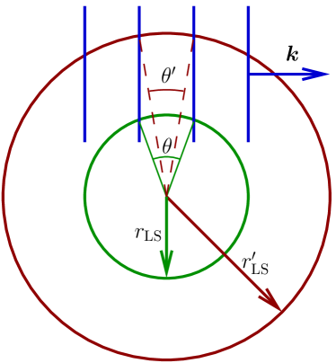
Figure 1: Our spheres of last scattering at time $\eta$ (inner) and $\eta^{\prime}$ (outer). The group of vertical lines indicates the crests of a mode ${\boldsymbol{k}}$, and hot spots will be observed at the intersections of those crests with the spheres. One wavelength of the mode will span angle $\theta$ at $\eta$ but a smaller angle $\theta^{\prime}$ at $\eta^{\prime}$.

We expand as usual the temperature fluctuation observed in some direction $\boldsymbol{\hat{e}}$ in terms of spherical harmonics $Y_{\ell m}$ as

$$\frac{\delta T(\boldsymbol{\hat{e}},\eta)}{T(\eta)}=\sum_{\ell m}a_{\ell m}(\eta)Y_{\ell m}(\boldsymbol{\hat{e}}).$$ (15)

The expansion coefficients $a_{\ell m}$ determine all the details of the particular sky map of the CMB observed at time $\eta$. However, the statistical properties of the $a_{\ell m}$s are determined through Eqs. (11) to (13) by the statistics of ${\cal R}$ encoded in Eq. (10). To make this explicit, we need the spherical expansion of the perturbations $\phi_{i}(r_{\rm LS},\boldsymbol{\hat{e}},\eta_{\rm LS})$, namely

$$\phi_{i}(r_{\rm LS},\boldsymbol{\hat{e}})=\sqrt{\frac{2}{\pi}}\int kdk\sum_{\ell m}\phi_{i\ell m}(k)j_{\ell}(kr_{\rm LS})Y_{\ell m}(\boldsymbol{\hat{e}}).$$ (16)

Here $i=1$ or $2$, $j_{\ell}$ is the spherical Bessel function of the first kind, and we have dropped the understood argument $\eta_{\rm LS}$. Next the identity

$$f_{\ell m}(k)=ki^{\ell}\int d\Omega_{\boldsymbol{k}}f({\boldsymbol{k}})Y_{\ell m}(\boldsymbol{\hat{k}})$$ (17)

(see, e.g., Ref. Liddle and Lyth (2000)) combined with Eq. (11) allows us to write

$$\phi_{i\ell m}(k)=A_{i}(k){\cal R}_{\ell m}(k).$$ (18)

Now, combining Eqs. (13), (16), and (18), we have

$$F(r_{\rm LS},\boldsymbol{\hat{e}})=\sqrt{\frac{2}{\pi}}\int kdk\sum_{\ell m}{\cal R}_{\ell m}(k)T(k,\ell,r_{\rm LS})Y_{\ell m}(\boldsymbol{\hat{e}}),$$ (19)

where

$$T(k,\ell,r_{\rm LS})\equiv A_{1}(k)j_{\ell}(kr_{\rm LS})+A_{2}(k)j_{\ell}^{\prime}(kr_{\rm LS})$$ (20)

and the prime denotes differentiation with resepect to $r_{\rm LS}$. Finally, equating coefficients between Eq. (19) [with Eq. (12)] and Eq. (15), we obtain

$$a_{\ell m}(\eta)=\sqrt{\frac{2}{\pi}}\int kdk{\cal R}_{\ell m}(k)T(k,\ell,r_{\rm LS}),$$ (21)

where we have restored the argument $\eta=r_{\rm LS}+\eta_{\rm LS}$. This expression gives the CMB anisotropy in terms of the primordial perturbations ${\cal R}$ and a new linear transfer function $T(k,\ell,r_{\rm LS})$.

In order to determine the statistical properties of the $a_{\ell m}$s, we need the expression

$$\langle{\cal R}_{\ell m}(k){\cal R}^{\ast}_{\ell^{\prime}m^{\prime}}(k^{\prime})\rangle=2\pi^{2}\delta(k-k^{\prime})\frac{{\cal P_{\cal R}}(k)}{k^{3}}\delta_{\ell\ell^{\prime}}\delta_{mm^{\prime}},$$ (22)

which can be derived from Eq. (10). Using this expression and Eq. (21) we find

$$\langle a_{\ell m}(\eta)a^{\ast}_{\ell^{\prime}m^{\prime}}(\eta)\rangle=C_{\ell}(\eta)\delta_{\ell\ell^{\prime}}\delta_{mm^{\prime}},$$ (23)

where

$$C_{\ell}(\eta)\equiv 4\pi\int\frac{dk}{k}{\cal P_{\cal R}}(k)T^{2}(k,\ell,r_{\rm LS}).$$ (24)

That is, each coefficient $a_{\ell m}$ has variance $C_{\ell}(\eta)$ (which is called the anisotropy power spectrum) and coefficients for different spherical modes are uncorrelated.

Note that Eq. (21), and hence Eqs. (23) and (24), hold even when we relax the tight coupling and free streaming approximations, with some transfer function $T(k,\ell,r_{\rm LS})$. However, in the general case the transfer function must be calculated numerically.

III.2 Analytical time evolution for primary anisotropies

The formalism developed in the preceeding subsection can now be applied to describe the time evolution of the primary CMB anisotropy spectrum, under the abrupt recombination and free streaming approximations. To determine the time evolution of $C_{\ell}(\eta)$, Eq. (24) tells us that we only need to consider the behaviour of $T^{2}(k,\ell,r_{\rm LS})$ as $r_{\rm LS}$ increases (note that we will often adopt the coordinate $r_{\rm LS}$ as an effective time coordinate). To do this, Eq. (20) tells us that we only require the behaviour of the products $j_{\ell}^{2}(kr_{\rm LS})$, $j_{\ell}^{\prime 2}(kr_{\rm LS})$, and $j_{\ell}(kr_{\rm LS})j_{\ell}^{\prime}(kr_{\rm LS})$ as functions of $r_{\rm LS}$. This can be done in the limit $\ell\gg 1$ using asymptotic forms for the Bessel functions. For large $\ell$ we can write [see Ref. Abramowitz and Stegun (1972), Eq. (9.3.3)]

$$j_{\ell}(x)=(x^{4}-x^{2}\ell^{2})^{-1/4}[\cos(\theta)+{\cal O}(1/\ell)],\quad\textrm{for }x>\ell,$$ (25)

where $\theta=\theta(x)$ is a real phase. For $x<\ell$, $j_{\ell}(x)$ decays rapidly. This allows us to write a scaling relation for the envelope of the Bessel oscillations, namely

$$j_{\ell}(x)\sim\alpha j_{\alpha\ell}(\alpha x),$$ (26)

for positive $\alpha$ such that $\alpha\ell\gg 1$ also applies. This expression will allow us to obtain the time dependence of the “monopole” contribution to $T^{2}(k,\ell,r_{\rm LS})$, which is proportional to $j_{\ell}^{2}(kr_{\rm LS})$. (The Bessel oscillations are rapid relative to the range of scales that contribute to the integral Eq. (24) for $\ell\gg 1$, and hence can be ignored.) We can write the “dipole” part $j_{\ell}^{\prime 2}(kr_{\rm LS})$ in terms of spherical Bessel functions using recurrence relations and again apply Eq. (26) to obtain the time dependence. The cross term proportional to $j_{\ell}(kr_{\rm LS})j_{\ell}^{\prime}(kr_{\rm LS})$ can be shown to be negligible, i.e. the monopole and dipole contributions add incoherently. Applying Eq. (26), then, we find that for large $\ell$,

$$T^{2}(k,\ell^{\prime},r_{\rm LS}^{\prime})\simeq\frac{r_{\rm LS}^{2}}{r_{\rm LS}^{\prime 2}}T^{2}(k,\ell,r_{\rm LS}),$$ (27)

where we have defined

$$\ell^{\prime}=\ell\frac{r_{\rm LS}^{\prime}}{r_{\rm LS}}.$$ (28)

Applying Eq. (24) we finally obtain the scaling relation for the power spectrum,

$$\ell^{\prime 2}C_{\ell^{\prime}}(\eta^{\prime})\simeq\ell^{2}C_{\ell}(\eta).$$ (29)

Importantly, Eq. (29) holds independently of the form of the functions $A_{i}(k)$ and ${\cal P_{\cal R}}(k)$, so the result applies to the acoustic peak structure as well as to non-scale-invariant primordial spectra.

This result confirms our previous prediction, Eq. (14), for the dependence of angular scales on observation time. But the dependence of the amplitude of the spectrum encoded in Eq. (29) is also not surprizing, since the quantity $\ell(\ell+1)C_{\ell}$ is independent of $\ell$ in the Sachs-Wolfe plateau for a scale invariant spectrum, as is well known. But the height of that plateau, calculated using $A_{1}={\rm const}$ and $A_{2}=0$ above, is independent of the observation time. (Indeed that height is, up to numerical factors, simply ${\cal P_{\cal R}}$. Recall that $C_{\ell}$ is determined by the ratio $\delta T/T$. The absolute anisotropies $\delta T$ exhibit the same expansion redshift as does the mean temperature $T$.) Hence as $\eta$ increases, the quantity $\ell^{2}C_{\ell}(\eta)$ must remain constant (up to corrections of order $1/\ell$), which is precisely what Eq. (29) says. Of course, the result (29) is valid for the entire acoustic peak structure, not just the Sachs-Wolfe plateau.

The result (29) is derived in the Appendix much more directly, without resorting to properties of Bessel functions, using the flat sky approximation. In that approach we consider anisotropies in a patch of sky small enough that it can be approximated as flat, and errors are again of order $1/\ell$.

In addition to the main temperature anisotropies we have been considering here, there are also polarization spectra present in the CMB radiation. The polarization is sourced primarily near last scattering, so its spectra will also scale according to Eq. (29). A small part of the largest-scale polarization is sourced near reionization, so we expect that that contribution will scale with the comoving radius to the reionization redshift, rather than to the last scattering surface.

Having found the scaling relation (29), we can next derive some simple consequences from it. First, we can write the total power in the anisotropy spectrum as

$$\sum_{\ell m}C_{\ell}(\eta)=\sum_{\ell}(2\ell+1)C_{\ell}(\eta)\simeq 2\int\ell C_{\ell}(\eta)d\ell$$ (30)

in the large $\ell$ approximation. Then, using Eq. (29), we have

$$\sum_{\ell}(2\ell+1)C_{\ell}(\eta)\simeq\sum_{\ell}(2\ell+1)C_{\ell}(\eta^{\prime}),$$ (31)

where the approximation comes from ignoring terms of order $1/\ell$. What this expression says is that the total power is constant in time, for the free streaming of primary anisotropies. This result is equivalent to the “conservation condition” stated in Bond and Efstathiou (1987). Implicit in this result is the assumption of statistical homogeneity, so that no new anomalous power will be revealed at the largest scales as $r_{\rm LS}$ increases. As we will see in Section III.3 below, secondary anisotropies, in particular those generated through the “integrated Sachs-Wolfe effect”, are expected to grow dramatically at late times and hence the total power will not in fact be conserved.

Another consequence of Eq. (29) follows from the nature of the asymptotic future in our $\Lambda$CDM model. Observers in a universe with positive $\Lambda$ have a future event horizon, i.e. the conformal time converges to a finite constant $\eta_{f}$ as proper time $t\rightarrow\infty$. Therefore the angular scaling relation (28) tells us that as proper time (or scale factor) approaches infinity, the $\ell$ value for any particular feature in the $C_{\ell}$ spectrum, such as a peak position, will approach a finite maximum, i.e. features will approach a non-zero minimum angular size. (Geometrically, the LSS sphere approaches a maximum comoving radius, so features on it must approach a minimum size.) For our fiducial model we chose $\Omega_{\Lambda}=0.77$, and so Eq. (28) gives for the limiting scaling relation

$$\ell_{f}=\ell_{0}\frac{\int_{a_{\rm LS}}^{\infty}(\dot{a}a)^{-1}da}{\int_{a_{\rm LS}}^{a_{0}}(\dot{a}a)^{-1}da}=1.31\ell_{0}.$$ (32)

For example, the first acoustic peak, which we observe to be at the position $\ell_{0}=221$ today, will asymptote to $\ell_{f}=290$ in the late de Sitter phase. This asymptotic behaviour is in marked contrast to that of a purely matter-dominated Einstein-de Sitter model. In the vanishing $\Lambda$ case, the numerator in Eq. (32) diverges (no event horizon exists) and the structure in the $C_{\ell}$ spectrum shifts to ever smaller scales.

The geometrical scaling relation (29) is very closely related to the well-known geometrical parameter degeneracy in the CMB anisotropy spectrum between spatial curvature and $\Lambda$ Bond et al. (1997); Zaldarriaga et al. (1997); Efstathiou and Bond (1999): If two cosmological models share the same primordial power spectrum ${\cal P_{\cal R}}(k)$, the same physical baryon and CDM densities today, $\rho_{b}$ and $\rho_{c}$, and finally the same angular diameter distance $d_{A}$ to the LSS, then they will exhibit essentially identical primary $C_{\ell}$ spectra. The degeneracy can only be broken by secondary sources of anisotropy, such as the integrated Sachs-Wolfe effect, or by other cosmological observations.

To understand the origin of this degeneracy and its relation to the preceeding discussion, recall that the energy density in the CMB today, $\rho_{\gamma}$, is fixed to very high accuracy by the measurement of the mean temperature, as we mentioned in the Introduction. Therefore if we consider models with identical values of the densities $\rho_{b}$ and $\rho_{c}$ today, then the densities of baryons, CDM, and photons at last scattering are the same for all such models, since the densities scale in a well-defined manner (for example, $\rho_{\gamma}/\rho_{c}\propto a_{0}/a$). Therefore, given the same initial conditions in the form of ${\cal P_{\cal R}}(k)$, models that have common values of $\rho_{b}$ and $\rho_{c}$ today will have identical local physics at least to the time of recombination, when any spatial curvature or $\Lambda$ will have negligible effect. Thus these models will produce identical primary anisotropies.

If the models have different values of $\Omega_{K}$ (spatial curvature) and $\Lambda$, then the dynamics, including the propagation of CMB anisotropies, will differ significantly at late times as those components come to dominate. However, if the models share the same angular diameter distance, then their $C_{\ell}$ spectra, which should be calculated using Eq. (24) with $r_{\rm LS}$ replaced by $d_{A}$ (at least for small scales where the effects of spatial curvature on the primordial spectra can be ignored), will be identical. Geometrically, models with identical ${\cal P_{\cal R}}(k)$, $\rho_{b}$, and $\rho_{c}$ share the same local physics to recombination, and hence the same physical scales for acoustic wave structures (in particular the same sound horizon). For models which additionally have identical $d_{A}$, observers see the anisotropies generated on a spherical shell at the time of last scattering of identical physical surface area (given by $4\pi d_{A}^{2}$). Hence those physical acoustic scales are mapped to identical angular scales in the sky for the different models. In short, the observed primary anisotropies in models with identical ${\cal P_{\cal R}}(k)$, $\rho_{b}$, $\rho_{c}$, and $d_{A}$ are produced under the same local physical conditions on a sphere of identical physical size, and hence appear identical. The scaling relation (29) describes how the observed anisotropies change if we hold the local physics at recombination (together with $\Lambda$ and $\Omega_{K}$) constant, but allow the time of observation to vary, which amounts to simply varying the size of the sphere at last scattering that generates the observed anisotropies. The parameter degeneracy states that the same anisotropy spectrum can be produced even if $\Lambda$ and $\Omega_{K}$ vary, as long as the size of the last scattering sphere is held constant.

To close this discussion of the primary anisotropies, we introduce the power spectrum difference $\delta C_{\ell}(\eta)\equiv C_{\ell}(\eta^{\prime})-C_{\ell}(\eta)$ between the spectra observed at two different times. This is a measurable quantity which we might consider a candidate for detecting the evolution of the CMB. Given some spectrum $C_{\ell}(\eta)$ at a single time $\eta$ we can readily calculate the difference $\delta C_{\ell}(\eta)$ using the scaling relation (29). For small $\delta\eta\equiv\eta^{\prime}-\eta$, we have

$$\delta C_{\ell}(\eta)\simeq\frac{\partial}{\partial\eta}C_{\ell}(\eta)\delta\eta,$$ (33)

so that the change in the CMB power spectrum at fixed $\ell$ is proportional to $\delta\eta$. As we will see in the next Section, this behaviour differs from that of the power spectrum of the difference $a_{\ell m}(\eta^{\prime})-a_{\ell m}(\eta)$. Using Eq. (29) for the time dependence, we can write

$$\delta C_{\ell}(\eta)=-\frac{\delta\eta}{\eta_{\rm LS}}\left[\ell\frac{\partial C_{\ell}(\eta)}{\partial\ell}+2C_{\ell}(\eta)\right],$$ (34)

at first order in $\delta\eta/\eta_{\rm LS}$. Note that $\delta C_{\ell}$ can have either sign, and will equal zero whenever $\partial(\ell^{2}C_{\ell})/\partial\ell=0$, as for example on a scale-invariant Sachs-Wolfe plateau or at an acoustic peak.

Recall that the quantity $C_{\ell}(\eta)$ describes the relative anisotropies $\delta T/T$, and hence is insensitive to the bulk expansion redshift. If we wish to consider instead the evolution of the absolute temperature anisotropies $\delta T$, the relevant quantity to calculate is

$$\delta[T^{2}C_{\ell}(\eta)]=T^{2}\left[-2\frac{\delta\eta}{(aH)^{-1}}C_{\ell}(\eta)+\delta C_{\ell}(\eta)\right]$$ (35)

at lowest order in $\delta\eta/(aH)^{-1}$, where we have used the relation $\dot{T}=-HT$. Since in standard $\Lambda$CDM models $\eta_{\rm LS}$ is a few times the comoving Hubble radius $(aH)^{-1}$, the first term on the left-hand side of Eq. (35) is of the same order as the second term. That is, the expansion cooling effect is on the same order as the geometrical scaling effect, and so it will be important to distinguish the two processes.

III.3 Integrated Sachs-Wolfe effect

The simple scaling relation derived in the previous subsection determines the time evolution of the power spectrum of anisotropies produced near the LSS. However, in the standard $\Lambda$CDM model, significant anisotropies are also produced at late times as a result of the changing equation of state as the Universe becomes cosmological constant dominated. This process is known as the (late) integrated Sachs-Wolfe (ISW) effect Sachs and Wolfe (1967); Kofman and Starobinsky (1985). Since these anisotropies are produced relatively locally, their time dependence must be explicitly calculated. Note that anisotropies are also generated by the early ISW effect, during the time that radiation still significantly contributes to the dynamics. However, those anisotropies are produced relatively close to the LSS, adding coherently to the primary Sachs-Wolfe contribution, and hence scale as do the primary anisotropies, according to Eq. (29).

The contribution of the late ISW effect can be described by adding to the transfer function, Eq. (20), a term $T_{\rm ISW}(k,\ell,\eta)$ which is an integral over the line of sight to the LSS. For the case of interest, for which the anisotropic stress is negligible, we have Dodelson (2003)

$$T_{\rm ISW}(k,\ell,\eta)=2A_{3}(k)\int_{\eta_{\rm LS}}^{\eta}d\eta^{\prime}g^{\prime}(\eta^{\prime})j_{\ell}[k(\eta-\eta^{\prime})].$$ (36)

Here $g^{\prime}(\eta)\equiv dg/d\eta$, with $g(\eta)$ being the growth function which describes the temporal evolution of the zero-shear or longitudinal gauge curvature perturbation, $\psi$ (also called the “Newtonian potential”), via

$$\psi(k,\eta)\equiv g(\eta)A_{3}(k){\cal R}(k).$$ (37)

The function $A_{3}(k)$ is defined such that $g(\eta)\rightarrow 1$ at early times in matter domination. Then, a gauge transformation between the comoving, ${\cal R}$, and zero-shear, $\psi$, curvature perturbations during the matter dominated period gives $A_{3}(k)=-3/5$.

To evaluate the ISW contribution, we need to first determine the evolution of the curvature perturbation $\psi$. To do this, we only need to solve the space-space, or dynamical, linearized Einstein equation. For the case where pressure and anisotropic stress perturbations can be ignored, which holds in a universe containing only dust and $\Lambda$, this equation becomes

$$\ddot{\psi}+4H\dot{\psi}+(3H^{2}+2\dot{H})\psi=0$$ (38)

(see, e.g., Ref. Mukhanov et al. (1992)). There are no spatial gradients in this equation, which confirms that the growth function is independent of $k$. It is straightforward to verify that the growing mode solution to this equation is

$$\psi(\eta)\propto\frac{H}{a}\int^{\eta}d\eta^{\prime}\frac{a^{2}\dot{H}}{H^{2}}.$$ (39)

Next, using the relation $a^{3}\dot{H}={\rm const}$, which holds exactly for a universe consisting of dust and cosmological constant, employing Eq. (37), and matching the growing mode solution to the initial condition $\psi_{0}(k)=-(3/5){\cal R}(k)$, we obtain

$$g(\eta)=\frac{5}{2}\frac{\Omega_{0}H}{a}\int^{\eta}\frac{d\eta^{\prime}}{aH^{2}},$$ (40)

where $\Omega_{0}$ is the density in matter today relative to the critical density, and the scale factor is normalized to unity today.

Now that the evolution of the growth function has been determined, we can evaluate the ISW contribution to the power spectrum. It can be shown that the cross term between the Sachs-Wolfe and (late) ISW terms is negligible, so the two add incoherently in $C_{\ell}$. For the ISW part we have

$$C_{\ell}^{\rm ISW}(\eta) = 4\pi\int\frac{dk}{k}{\cal P_{\cal R}}(k)T_{\rm ISW}^{2}(k,\ell,\eta)$$ (41)

$$= \frac{72}{25}\frac{\pi^{2}{\cal P_{\cal R}}}{\ell^{3}}\int_{0}^{\eta}d\eta^{\prime}g^{\prime 2}(\eta^{\prime})(\eta-\eta^{\prime}).$$ (42)

To obtain this result we have assumed a scale invariant primordial spectrum, ${\cal P_{\cal R}}(k)={\cal P_{\cal R}}$, and we have used the relation Kamionkowski and Spergel (1994)

$$\int_{0}^{\infty}\frac{dk}{k}j_{\ell}[k(\eta-\eta^{\prime})]j_{\ell}[k(\eta-\eta^{\prime\prime})]\simeq\frac{\pi}{2\ell^{3}}(\eta-\eta^{\prime})\delta(\eta^{\prime}-\eta^{\prime\prime}),$$ (43)

which holds for large $\ell$. Unfortunately it is at small $\ell$ that the ISW effect is greatest, so this approximation, which appears to be the best we can do analytically, is not terribly accurate at very late times, when, as we shall see, the ISW contribution becomes very large. Nevertheless, Eq. (42) will give a reasonable estimate of the ISW contribution to a change $\delta C_{\ell}$ over short time intervals.

Given a primordial amplitude, ${\cal P_{\cal R}}$, and a matter density parameter today, $\Omega_{0}$, Eqs. (40) and (42) allow us to calculate the ISW contribution to the power spectrum at any time. In addition, taking the time derivative of Eq. (42), we find for the rate of change of the ISW contribution

$$\frac{\partial}{\partial\eta}C_{\ell}^{\rm ISW}(\eta)=\frac{72}{25}\frac{\pi^{2}{\cal P_{\cal R}}}{\ell^{3}}\int_{0}^{\eta}d\eta^{\prime}g^{\prime 2}(\eta^{\prime}).$$ (44)

Therefore, combining this expression with Eq. (34) for the change in the primary Sachs-Wolfe power spectrum over short time intervals $\delta\eta$, we find for the total contribution

$$\delta C_{\ell}(\eta)= - \frac{\delta\eta}{\eta_{\rm LS}}\left[\ell\frac{\partial C_{\ell}(\eta)}{\partial\ell}+2C_{\ell}(\eta)\right.$$ (45)

$$- \left.\frac{72}{25}\frac{\pi^{2}{\cal P_{\cal R}}}{\ell^{3}}\eta_{\rm LS}\int_{0}^{\eta}d\eta^{\prime}g^{\prime 2}(\eta^{\prime})\right].$$

III.4 Gravitational waves

Inflationary models generically predict a spectrum of primordial gravitational waves, although the relative contribution of these tensor modes to the total CMB anisotropy ranges from substantial to very small, depending on the model. The anisotropies arise through the tensor analogue of the scalar ISW line of sight integral, Eq. (36). In place of the time derivative of the scalar curvature perturbation $\psi$, the tensor contribution involves the rate of change of the transverse and traceless part of the spatial metric perturbation, $h_{ij}$. The evolution of this part of the metric perturbation is given by the dynamical Einstein equation, which becomes (see, e.g., Mukhanov et al. (1992))

$$h_{ij}^{\prime\prime}+2aHh_{ij}^{\prime}-\nabla^{2}h_{ij}=0$$ (46)

in the absence of tensor anisotropic stress, which is a valid approximation in the matter- or $\Lambda$-dominated regimes.

The dynamics of $h_{ij}$ as dictated by this equation depends on the mode wavelength relative to the Hubble scale. For $k/(aH)\ll 1$, the tensor mode is overdamped, and the (growing) mode decays very slowly. For $k/(aH)\gg 1$, the mode undergoes underdamped oscillations, decaying like $h_{ij}\propto e^{ik\eta}/a$ in the adiabatic regime. Therefore, for a particular tensor mode $k$, the rate of change $h_{ij}^{\prime}$ is peaked near the time that the mode crosses the Hubble radius, $k/(aH)\sim 1$, and is small at early and late times. This means that the contributions to the CMB anisotropies from a particular scale arise primarily when that scale enters the Hubble radius. In particular, scales that enter significantly before last scattering will have decayed before they could source the CMB. This imposes a small scale cut-off on the tensor anisotropy spectrum, with negligible power for

$$\ell\gg\ell_{c}\equiv r_{\rm LS}\dot{a}_{\rm LS},$$ (47)

where $1/\dot{a}_{\rm LS}$ is the comoving Hubble radius at last scattering. Since $\dot{a}_{\rm LS}$ is fixed for a particular model, the $\ell$ cut-off scales with time of observation according to

$$\ell_{c}(\eta^{\prime})=\ell_{c}(\eta)\frac{r_{\rm LS}^{\prime}}{r_{\rm LS}},$$ (48)

which is the same scaling as for primary features in the scalar CMB spectrum, Eq. (28).

For $\ell\ll\ell_{c}$, detailed calculations for a matter dominated universe Starobinsky (1985); Turner et al. (1993) show that the tensor anisotropy spectrum is nearly flat, mimicing the Sachs-Wolfe plateau. In this case the tensor spectrum does not evolve apart from the scaling of the cut-off, Eq. (48). However, as described above, the largest angular scales will be sourced at the latest times, and so for a universe with cosmological constant this will lead to some dependence on observation time for those scales as the equation of state changes at late times. For example, for time of observation $\eta$ the tensor quadrupole is sourced near very roughly the conformal time $\eta/2$ Starobinsky (1985). In the matter-dominated era, the comoving Hubble radius $1/(aH)=1/\dot{a}$ increases with time, but as the Universe enters the $\Lambda$-dominated era, $1/(aH)$ starts to decrease (indeed this defines acceleration). Therefore, the largest scale modes that contribute to the tensor anisotropies will enter the Hubble radius somewhat later in the presence of a cosmological constant than without (sufficiently large-scale modes will never enter the Hubble radius). The modes which enter near time $\eta_{f}/2$, where $\eta_{f}$ is the asymptotic final conformal time, will have a significantly delayed entry time, and therefore we expect the very largest scale tensor anisotropies to be somewhat reduced at the latest times.

III.5 Optical depth

One final line of sight effect on the CMB anisotropies that we will consider is the time dependent optical depth due to Thomson scattering. Looking back, it is the rapid increase in scattering near the time of recombination that makes it possible to speak of a “surface of last scattering”, where the primary anisotropies are emitted. At later times, reionization results in a time dependent attenuation of the amplitude of the power spectrum, which it will be important to quantify.

In our fiducial model the epoch of reionization occurs at redshift $z_{R}=11.1$, or $a_{R}=0.083$, with the scale factor normalized to unity today. Here, we see a decrease in the amplitude of intermediate to small scale ($\ell\gtrsim 30$) anisotropies as photons are rescattered. On these scales, $C_{\ell}(\eta)$ is reduced by a factor $e^{2\tau_{R}}$, where $\tau_{R}$ is the optical depth to reionization. To compute the suppression in $C_{\ell}(\eta)$, recall the definition of the optical depth $\tau(a,a_{\rm obs})$ between scale factors $a$ and $a_{\rm obs}$, given by

$$\tau(a,a_{\rm obs})=\sigma_{\rm T}\int^{a_{\rm obs}}_{a}\frac{dt}{da^{\prime}}\,n_{e}(a^{\prime})\,da^{\prime}\,,$$ (49)

where $\sigma_{\rm T}$ is the Thomson scattering cross-section and $n_{e}(a)$ the electron number density. Assuming reionization is sharp and the energy density of radiation is subdominant, the optical depth to reionization, $\tau_{R}(a_{\rm obs})\equiv\tau(a_{R},a_{\rm obs})$ is given by (see, e.g., Griffiths et al. (1999))

$$\tau_{\rm R}(a_{\rm obs})=0.046(1-Y_{p})\!\!\!\!\!\!\!\! \frac{\Omega_{b}}{\Omega_{m}}\left(\sqrt{\Omega_{m}h^{2}a_{R}^{-3}+\Omega_{\Lambda}h^{2}}\right.$$ (50)

$$- \left.\sqrt{\Omega_{m}h^{2}a_{\rm obs}^{-3}+\Omega_{\Lambda}h^{2}}\right),$$

with $\tau_{R}(a_{\rm obs})=0$ for $a_{\rm obs}\leq a_{R}$. In this expression $Y_{p}$ is the primordial helium fraction (assumed to be 0.24).

Eq. (50) gives $\tau_{R}(1)=0.088$, so reionization reduces $C_{\ell}(\eta)$ by a factor of approximately $0.84$ by today [of course we must evaluate the spectrum at different times at the $\ell$ values related by the scaling relation Eq. (28)]. Much of the suppression of $C_{\ell}(\eta)$ occurs before the present time. Since the time the scale factor was half its present value, for example, the optical depth to reionization has only increased by $0.003$. As $a_{\rm obs}\rightarrow\infty$, Eq. (50) says that the optical depth will only increase by $\delta\tau_{\infty}\equiv\tau_{R}(\infty)-\tau_{R}(1)=5.7\times 10^{-4}$, so that $C_{\ell}(\eta)$ will only be reduced by $0.1\%$ relative to the value today. (Note that the peak positions should not be effected by reionization, since the peak structure is at scales smaller than those corresponding to the particle horizon at rescattering.) Therefore the Universe is essentially transparent on cosmological scales today, and we have already seen nearly the maximum amount of reionization damping.

III.6 Time evolution from CAMB

In order to confirm and extend the analytic results of previous subsections we have modified the camb software Lewis et al. (2000) to compute the CMB power spectrum at different observational times. To do this, we simply modify all routines such that we can evaluate the transfer functions $T(k,\ell,r_{\rm LS})$ at different $r_{\rm LS}$, using the set of best-fitting cosmological parameters as measured today. The changes required to camb are straightforward—for the most part all that is needed is to change the tau0 variable to trick the code into using a different observational time. The parameters we use are those of a standard six parameter spatially flat $\Lambda$CDM model, given by $\Omega_{c}h^{2}=0.104$, $\Omega_{b}h^{2}=0.0223$, $h=0.734$, $n_{S}=0.951$, $A_{S}=2.02\times 10^{-9}$, and $z_{R}=11.1$, where ${\cal P_{\cal R}}(k)=A_{S}(k/k_{0})^{n_{S}-1}$ with pivot scale $k_{0}=0.05\,{\rm Mpc}^{-1}$, and $z_{R}$ is the redshift of reionization. Where necessary, we set $n_{S}=1$ to simplify comparison with analytic results. We do not expect significant differences in our results if these parameters are varied somewhat. Since the parameters are defined relative to their present day values, the spectrum measured by an observer with $z>z_{R}$, for example, will not be affected by the epoch of reionization and a future observer will see a universe completely dominated by dark energy.

In Fig. 2 we plot the power spectrum $\ell(\ell+1)C_{\ell}(\eta)/(2\pi)$ calculated from our modified version of camb, parameterizing the time dependence in terms of the observational scale factor $a_{\rm obs}$, where $a_{\rm obs}=1$ corresponds to today. It is clear that the angular scale of features resulting from projection of inhomogeneities near the LSS can be understood from the scaling relation (29). For example, in Fig. 2 we show the predicted scaling of the first acoustic peak position (located at $\ell=221$ at the present time) and find extremely good agreement with the predicted value. The existence of a future event horizon means that during $\Lambda$ domination $dr_{\rm LS}/da_{\rm obs}$ tends to zero and so the acoustic peak positions become “frozen in”. With our parameters we see that the first acoustic peak becomes frozen in at the value $\ell_{f}\simeq 290$ as we predicted in Eq. (32).

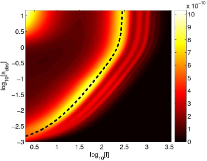
Figure 2: CMB power spectrum $\ell(\ell+1)C_{\ell}/(2\pi)$ as a function of multipole $\ell$ and scale factor of observation $a_{\rm obs}$, as calculated from our modified version of camb for our fiducial $\Lambda$CDM model. We also plot the analytic scaling of the first acoustic peak (thick dashed line) predicted by Eq. (29).

Recall that the scaling relation Eq. (29) predicts not only how the angular sizes of features in the spectrum scale with time, but also that the magnitude of the power, $\ell(\ell+1)C_{\ell}(\eta)$, remains constant into the future at, e.g., any acoustic peak. For late times, $a_{\rm obs}\gtrsim 0.3$, Fig. 2 indeed confirms this prediction. Our fiducial model underwent reionization at $a_{R}=0.083$, and we predicted in Section III.5 that as a result the power spectrum should be attenuated by approximately $16\%$ on all but the largest scales. Again, this is visible in Fig. 2. Recall that we predicted a negligible $0.1\%$ reduction in $C_{\ell}(\eta)$ between today and the distant future.

Also visible in Fig. 2 is a substantial increase in power at the largest scales at late times due to the increasing ISW effect in our $\Lambda$CDM model, which we discussed in Section III.3. Indeed, for $a_{\rm obs}\gtrsim 5.0$ the quadrupole power actually exceeds the power at the first acoustic peak. The ISW contribution converges as the observation scale factor $a_{\rm obs}$ approaches infinity, since in the integral in Eq. (42), we have $g^{\prime}(\eta)\rightarrow 0$ and $\eta\rightarrow\eta_{f}$ as $a_{\rm obs}\rightarrow\infty$, where $\eta_{f}$ is finite. The asymptotic form of the power spectrum at late times is plotted in Fig. 3, together with the current spectrum. The dramatic increase in the ISW contribution, as well as the shift in peak positions predicted in Eq. (32), are clearly visible. Note that the ISW contribution to the dipole power, though not shown in Fig. 3, asymptotes to $C_{1}^{\rm ISW}(\eta_{f})\simeq 5\times 10^{-9}$ for out model, according to camb. This corresponds to typical dipole ISW amplitudes $a_{1m}^{\rm ISW}\simeq\sqrt{C_{1}^{\rm ISW}}\simeq 7\times 10^{-5}$. Although such amplitudes represent a large increase over the current ISW dipole, they are still considerably below either the current total measured dipole, $a_{10}=2.5\times 10^{-3}$ (with the polar axis aligned with the dipole), or the amplitude of the galactic orbital dipole oscillation, $a_{10}=1.5\times 10^{-3}$ according to Eq. (8).

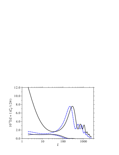
Figure 3: Anisotropy power spectra for scalars (top pair of curves) and for tensors (bottom pair, arbitrary scale), calculated using our modified version of camb for today (dashed curves) and for the asymptotic future (solid).

Fig. 3 also presents the gravitational wave contribution to the anisotropy spectra today and in the asymptotic future. In Section III.4 we described the expected behaviour of tensor modes in the future, which entailed the same geometrical scaling of the small-scale cut-off in the spectrum, as well as a decrease in power at the very largest scales. Both of these features are visible in Fig. 3.

As a check on our custom modifications to camb, we plot in Fig. 4 the power spectrum from camb for $a_{\rm obs}=2.0$, as well as the corresponding curve calculated from a power spectrum generated for today, $a_{\rm obs}=1$, and transformed to $a_{\rm obs}=2.0$ using the scaling relation Eq. (29). Additionally, the spectrum calculated from the scaling relation includes the increased ISW component calculated from the analytical approximation Eq. (42). To facilitate the use of this analytical expression, the spectral index was set to $n_{S}=1$ for these calculations. Since the curves coincide at all but the largest scales, it is clear that the scaling relation has accurately captured the evolution of $C_{\ell}(\eta)$. However, the ISW contribution is substantially overestimated, indicating the limitations of the approximation Eq. (43) involved in deriving Eq. (42).

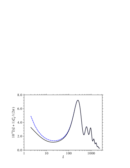
Figure 4: Anisotropy power spectrum for $a_{\rm obs}=2.0$ calculated with our modified version of camb (solid line) and using the scaling relation Eq. (29) and analytical ISW approximation Eq. (42) (dashed). We set $n_{S}=1$ for these calculations.

To make further contact with the analytic results in previous subsections, in Fig. 5 we plot the difference $\delta C_{\ell}\equiv C_{\ell}(a^{\prime}_{\rm obs})-C_{\ell}(a_{\rm obs})$ calculated using our modified version of camb between the power spectrum today, at $a_{\rm obs}=1$, and at a future time, when $a^{\prime}_{\rm obs}=1+\delta a$, for the cases $\delta a=10^{-4}$, $0.001$, and $0.01$. These curves exhibit very accurately the scaling with $\delta a$ predicted in Eq. (33), when we recall that $\delta a=H_{0}\delta\eta$ for small $\delta\eta$. Slight departures from this simple scaling are evident at the largest scales, where the spectra are nearly flat and hence their precise shape sensitively influences the location of zeros in $\delta C_{\ell}$. In Fig. 5 we also plot the analytical result calculated from the power spectrum today using Eq. (45). Again we find excellent agreement with camb at all but the largest scales. We also find reasonable agreement at low $\ell$, indicating that our ISW approximation is quite good for small time increments from today.

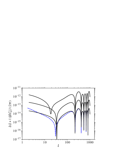
Figure 5: Absolute value of the difference in the CMB power spectra $\ell(\ell+1)|\delta C_{\ell}|/(2\pi)$ between $a_{\rm obs}=1$ and $a^{\prime}_{\rm obs}=1+\delta a$. The solid curves were calculated from our modified version of camb, and from top to bottom denote $\delta a=0.01$, $0.001$, and $10^{-4}$. The dashed curve was calculated using the analytical expression Eq. (45) for $\delta a=10^{-4}$. We used $n_{S}=1$ for these calculations.

IV The difference map power spectrum

IV.1 Analytical time evolution

In the previous section we found a very simple scaling relation to describe the time dependence of the CMB power spectrum, which, together with the ISW effect, thoroughly describes the evolution of the spectrum. However, if we are interested in the best way to observe evolution in the CMB we might expect that observing changes in the actual sky map, or the $a_{\ell m}$s, should be far more promising than looking for changes in the heavily compressed $C_{\ell}$ power spectrum. Intuitively, as the shell $r=r_{\rm LS}$ of the LSS grows in size, we expect the finest structures to change first, then the larger ones. As we shall see, the difference between two sky maps measured at different times does indeed encode much more information than the $C_{\ell}$ spectra, namely the correlations between the two maps, although perhaps counterintuitively the magnitude of a change $C_{\ell}$ will dominate over the difference map power spectrum for small time intervals.

IV.1.1 Definitions

Consider two measurements of the $a_{\ell m}$s at times $\eta$ and $\eta^{\prime}$ and define the difference map by

$$\delta a_{\ell m}\equiv a_{\ell m}(\eta^{\prime})-a_{\ell m}(\eta).$$ (51)

Using Eq. (21), we can readily calculate the statistical properties of the difference map. We find

$$\langle\delta a_{\ell m}\delta a^{\ast}_{\ell^{\prime}m^{\prime}}\rangle=D_{\ell}^{\eta\eta^{\prime}}\delta_{\ell\ell^{\prime}}\delta_{mm^{\prime}},$$ (52)

where we define the power spectrum of the difference map, $D_{\ell}^{\eta\eta^{\prime}}$, by

$$D_{\ell}^{\eta\eta^{\prime}}\equiv C_{\ell}(\eta)+C_{\ell}(\eta^{\prime})-2C_{\ell}^{\eta\eta^{\prime}},$$ (53)

and

$$C_{\ell}^{\eta\eta^{\prime}}\equiv 4\pi\int\frac{dk}{k}{\cal P_{\cal R}}(k)T(k,\ell,r_{\rm LS})T(k,\ell,r_{\rm LS}^{\prime}).$$ (54)

Note that the quantity $\langle\delta a_{\ell m}\delta a^{\ast}_{\ell^{\prime}m^{\prime}}\rangle$ is diagonal in $\ell$ and $m$, and that $C_{\ell}^{\eta\eta}=C_{\ell}(\eta)$.

The quantity $C_{\ell}^{\eta\eta^{\prime}}$ is an unequal time correlator, i.e. a correlation function that relates the anisotropies at time $\eta$ with those at time $\eta^{\prime}$, through

$${\rm Re}\,\langle a_{\ell m}(\eta)a^{\ast}_{\ell^{\prime}m^{\prime}}(\eta^{\prime})\rangle=C_{\ell}^{\eta\eta^{\prime}}\delta_{\ell\ell^{\prime}}\delta_{mm^{\prime}}.$$ (55)

Since the variances $C_{\ell}(\eta)$ and $C_{\ell}(\eta^{\prime})$ will in general differ, the quantity $C_{\ell}^{\eta\eta^{\prime}}$ is not the best measure of correlations, and the spectrum $D_{\ell}^{\eta\eta^{\prime}}$ measures not only the loss of correlations but also the change in variance $C_{\ell}(\eta)$. Therefore we may consider instead the modified difference map

$$\overline{\delta a}_{\ell m}\equiv\sqrt{\frac{C_{\ell}(\eta)}{C_{\ell}(\eta^{\prime})}}a_{\ell m}(\eta^{\prime})-a_{\ell m}(\eta),$$ (56)

which normalizes the modes at $\eta^{\prime}$ to have the same variance as those at $\eta$. Then we find

$$\langle\overline{\delta a}_{\ell m}\overline{\delta a}{}^{\ast}_{\ell^{\prime}m^{\prime}}\rangle=2C_{\ell}(\eta)\left(1-\bar{C}_{\ell}^{\eta\eta^{\prime}}\right)\delta_{\ell\ell^{\prime}}\delta_{mm^{\prime}},$$ (57)

where we have defined the normalized correlation function by

$$\bar{C}_{\ell}^{\eta\eta^{\prime}}\equiv\frac{C_{\ell}^{\eta\eta^{\prime}}}{\sqrt{C_{\ell}(\eta)C_{\ell}(\eta^{\prime})}}.$$ (58)

This normalized function is useful in that we have $\bar{C}_{\ell}^{\eta\eta^{\prime}}=1$, $0$, and $-1$ for perfect correlations, no correlations, and perfect anticorrelations, respectively. Similarly, the quantity $1-\bar{C}_{\ell}^{\eta\eta^{\prime}}$ measures the loss of correlations alone. However, the spectrum $D_{\ell}^{\eta\eta^{\prime}}$ will still be useful, since it measures both the loss of correlations and the change in variance, so it might be expected to be more sensitive to changes in the CMB than the quantity $1-\bar{C}_{\ell}^{\eta\eta^{\prime}}$. Also, through the definition (51), the quantity $D_{\ell}^{\eta\eta^{\prime}}$ is more directly tied to observations.

IV.1.2 Time evolution—flat sky approximation

In analogy with Eq. (33) for $\delta C_{\ell}$, we can write the spectrum of the difference map for small increments in time $\delta\eta=\eta^{\prime}-\eta$ as

$$D_{\ell}^{\eta\eta^{\prime}}\simeq\left\langle\frac{\partial a_{\ell m}}{\partial\eta}\frac{\partial a_{\ell m}^{\ast}}{\partial\eta}\right\rangle(\delta\eta)^{2}.$$ (59)

Therefore the difference of the power spectrum, $\delta C_{\ell}$, dominates over the power spectrum of the difference map, $D_{\ell}^{\eta\eta^{\prime}}$, for small enough $\delta\eta$, since $\delta C_{\ell}$ is only proportional to the first power of $\delta\eta$. Of course for a particular $\delta\eta$ we must calculate the coefficients of $\delta\eta$ and $(\delta\eta)^{2}$ before we decide which method is more efficient if we are interested in a detection. The details of instrumental noise are important and this is discussed fully in Moss et al. (2007).

Beyond the $(\delta\eta)^{2}$ scaling, it is much more difficult to obtain the detailed evolution of $D_{\ell}^{\eta\eta^{\prime}}$ than it was for $\delta C_{\ell}$. Even when we consider only the Sachs-Wolfe plateau contribution, for which $A_{1}(k)=-1/5$ and $A_{2}(k)=A_{3}(k)=0$, the Bessel integrals involved in Eq. (54) cannot be analytically solved. In fact, this problem is related to a divergence that can be illuminated if we employ the flat sky approximation described in the Appendix.

Under that approximation, which is valid over small patches of sky and replaces the discrete indices $\ell$ and $m$ with the continuous two-dimensional vector ${\boldsymbol{\ell}}$, and the polar coordinate $r$ with a Cartesian coordinate $x$ parallel with the line of sight, we can readily calculate the quantity on the left-hand side of Eq. (52). Using

$$\delta a({\boldsymbol{\ell}})\equiv a({\boldsymbol{\ell}},x_{\rm LS}^{\prime})-a({\boldsymbol{\ell}},x_{\rm LS})$$ (60)

to define the difference map, where $x_{\rm LS}$ and $x_{\rm LS}^{\prime}$ are the comoving distances to the LSS at times $\eta$ and $\eta^{\prime}$, respectively, and using Eq. (95) for the anisotropies, we find that the result is not diagonal in ${\boldsymbol{\ell}}$. Rather, it contains terms proportional to the Dirac functions $\delta^{2}(\alpha{\boldsymbol{\ell}}-{\boldsymbol{\ell}}\,^{\prime})$ and $\delta^{2}(\alpha^{-1}{\boldsymbol{\ell}}-{\boldsymbol{\ell}}\,^{\prime})$, where we have defined

$$\alpha\equiv\frac{x_{\rm LS}^{\prime}}{x_{\rm LS}}.$$ (61)

Indeed this is not surprizing: in the flat sky approximation, an anisotropy on angular scale ${\boldsymbol{\ell}}$ at $x_{\rm LS}$ corresponds to a physical mode with comoving wavevector component ${\boldsymbol{\ell}}/x_{\rm LS}$ orthogonal to the line of sight. But Eq. (10) tells us that such a mode should share correlations with the same physical scale at $x_{\rm LS}^{\prime}$, which corresponds to the angular scale ${\boldsymbol{\ell}}x_{\rm LS}^{\prime}/x_{\rm LS}$. Such off-diagonal correlations are completely suppressed in the full spherical expansion, as we found.

The relevant quantity to calculate in the flat sky approximation is instead the power in the difference map defined by

$$\widetilde{\delta a}({\boldsymbol{\ell}})\equiv a(\alpha{\boldsymbol{\ell}},x_{\rm LS}^{\prime})-a({\boldsymbol{\ell}},x_{\rm LS}).$$ (62)

Again applying Eq. (95) for $a({\boldsymbol{\ell}},x_{\rm LS})$, we find

$$\left\langle\widetilde{\delta a}({\boldsymbol{\ell}})\widetilde{\delta a}{}^{\ast}({\boldsymbol{\ell}}\,^{\prime})\right\rangle=D^{\eta\eta^{\prime}}\!({\boldsymbol{\ell}})\,\delta^{2}({\boldsymbol{\ell}}-{\boldsymbol{\ell}}\,^{\prime}),$$ (63)

which is diagonal in ${\boldsymbol{\ell}}$, with the power spectrum of the difference map given by

$$D^{\eta\eta^{\prime}}\!({\boldsymbol{\ell}})\equiv C({\boldsymbol{\ell}},\eta)+\alpha^{-2}C(\alpha{\boldsymbol{\ell}},\eta^{\prime})-2C^{\eta\eta^{\prime}}\!({\boldsymbol{\ell}}).$$ (64)

Here $C({\boldsymbol{\ell}},\eta)$ is the flat sky approximation to the anisotropy power spectrum, given by Eq. (98), and $C^{\eta\eta^{\prime}}\!({\boldsymbol{\ell}})$ is the correlation function given by

$$C^{\eta\eta^{\prime}}\!({\boldsymbol{\ell}})\equiv\frac{\pi}{x_{\rm LS}^{\prime 2}}\!\int_{-\infty}^{\infty}\!\!\!\!\!dk_{x}\!\frac{{\cal P_{\cal R}}(k)|T(k,k_{x})|^{2}\cos(k_{x}\delta x_{\rm LS})}{k^{3}},$$ (65)

where $T(k,k_{x})$ is the flat sky transfer function, $\delta x_{\rm LS}\equiv x_{\rm LS}^{\prime}-x_{\rm LS}$, and $k_{x}$ is the component of the comoving wavevector parallel to the line of sight. Eqs. (62) to (65) are the flat sky analogues of Eq. (51) to (54), respectively. (The continuous argument $({\boldsymbol{\ell}})$ will always distinguish quantities in the flat sky approximation from the corresponding exact quantities, which are labelled with the discrete indices _ℓm.)

Note that the integrand in Eq. (65), which is exact apart from the flat sky approximation, is bounded in magnitude by the integrand in Eq. (98) for the power spectrum $C({\boldsymbol{\ell}},\eta)$, as we vary $\delta x_{\rm LS}$. In place of Eq. (58), the normalized correlation function becomes in the flat sky approximation

$$\bar{C}^{\eta\eta^{\prime}}\!({\boldsymbol{\ell}})\equiv\frac{C^{\eta\eta^{\prime}}\!({\boldsymbol{\ell}})}{\sqrt{C({\boldsymbol{\ell}},\eta)\alpha^{-2}C(\alpha{\boldsymbol{\ell}},\eta^{\prime})}},$$ (66)

which is bounded by $|\bar{C}^{\eta\eta^{\prime}}\!({\boldsymbol{\ell}})|\leq 1$. In the limit of short time interval, $\delta x_{\rm LS}\rightarrow 0$, we have $\bar{C}^{\eta\eta^{\prime}}\!({\boldsymbol{\ell}})\rightarrow 1$, corresponding to perfect correlation. We also have $\bar{C}^{\eta\eta^{\prime}}\!({\boldsymbol{\ell}})\rightarrow 0$ as $\delta x_{\rm LS}\rightarrow\infty$ (recall, however, that in a $\Lambda$CDM universe, only finite conformal time is available into the future).

IV.1.3 Special cases

Armed with the above flat sky approximation, we can now calculate the difference map power spectrum and correlation function in some special cases. First, consider the short time interval case, $\delta x_{\rm LS}\rightarrow 0$. Expanding Eq. (64) in powers of $k_{x}\delta x_{\rm LS}\sim\ell\delta x_{\rm LS}/x_{\rm LS}$, where $\ell\equiv|{\boldsymbol{\ell}}|$, we find

$$D^{\eta\eta^{\prime}}\!({\boldsymbol{\ell}})=\pi\left(\frac{\delta x_{\rm LS}}{x_{\rm LS}}\right)^{2}\!\!\int_{-\infty}^{\infty}\!\!dk_{x}\frac{{\cal P_{\cal R}}(k)|T(k,k_{x})|^{2}k_{x}^{2}}{k^{3}}$$ (67)

for the power spectrum of the difference map at lowest order in $\ell\delta x_{\rm LS}/x_{\rm LS}$. This expression exhibits precisely the time interval dependence that we predicted in Eq. (59). (Note that in defining the difference map through Eq. (62), we have fixed the observed transverse wavevectors at both observation times, so the integrand in Eq. (67) is independent of $\delta\eta$.)

The integrand in Eq. (67) resembles closely that for the anisotropy power spectrum in Eq. (98), but with an extra factor of $k_{x}^{2}$ in the numerator. In fact, using the relation

$$k^{2}=k_{x}^{2}+\left(\frac{\ell}{x_{\rm LS}}\right)^{2}$$ (68)

we can easily rewrite Eq. (67) as

$$D^{\eta\eta^{\prime}}\!({\boldsymbol{\ell}})=\left(\frac{\delta x_{\rm LS}}{x_{\rm LS}}\right)^{2}\!\left[\ell_{0}^{2}C^{(n_{S}+2)}({\boldsymbol{\ell}},\eta)-\ell^{2}C({\boldsymbol{\ell}},\eta)\right].$$ (69)

Here $C^{(n_{S}+2)}({\boldsymbol{\ell}},\eta)$ is the anisotropy power spectrum calculated using a modified primordial power spectrum defined by

$${\cal P}_{\cal R}^{(n_{S}+2)}(k)\equiv\left(\frac{k}{k_{0}}\right)^{2}{\cal P_{\cal R}}(k),$$ (70)

where $k_{0}\equiv\ell_{0}/x_{\rm LS}$ is the “pivot scale” used to define the primordial spectrum. (The result for $D^{\eta\eta^{\prime}}\!({\boldsymbol{\ell}})$ is, of course, independent of the pivot scale chosen.) For the special case of a power law primordial spectrum ${\cal P_{\cal R}}(k)$, with scalar spectral index $n_{S}$, the modified spectrum ${\cal P}_{\cal R}^{(n_{S}+2)}(k)$ has spectral index $n_{S}+2$; hence our choice of notation. Eq. (69) says that, for small time increments, the shape of the power spectrum of the difference map is determined entirely by the actual anisotropy spectrum “blue tilted”, i.e. $\ell^{2}C({\boldsymbol{\ell}},\eta)$, together with the spectrum $C^{(n_{S}+2)}({\boldsymbol{\ell}},\eta)$ calculated from a blue-tilted primordial spectrum, both evaluated at the same time $\eta$. Therefore we expect that generically the shape of the difference map spectrum $D^{\eta\eta^{\prime}}\!({\boldsymbol{\ell}})$ will be roughly that of a strongly blue-tilted version of the anisotropy spectrum $C({\boldsymbol{\ell}},\eta)$. The height of the spectrum of the difference map is determined by the ratio $\delta x_{\rm LS}/x_{\rm LS}$.

Next, we can specialize to the case of the pure scale-invariant ($n_{S}=1$) Sachs-Wolfe plateau, which is characterized by $T(k,k_{x})=A_{1}(k)={\rm const}$ and ${\cal P_{\cal R}}(k)={\rm const}$. Eq. (98) gives in this case

$$C({\boldsymbol{\ell}},\eta)=\frac{2\pi{\cal P_{\cal R}}A_{1}^{2}}{\ell^{2}},$$ (71)

in agreement with the standard Sachs-Wolfe result, to order $1/\ell$. The normalized correlation function is then

$$\bar{C}^{\eta\eta^{\prime}}\!({\boldsymbol{\ell}})=\frac{\ell^{2}}{2x_{\rm LS}^{2}}\int_{-\infty}^{\infty}dk_{x}\frac{\cos(k_{x}\delta x_{\rm LS})}{k^{3}}.$$ (72)

In the short time interval limit, $\ell\delta x_{\rm LS}/x_{\rm LS}\ll 1$, Eq. (67) becomes for the Sachs-Wolfe plateau

$$D^{\eta\eta^{\prime}}\!({\boldsymbol{\ell}})=\pi{\cal P_{\cal R}}A_{1}^{2}\left(\frac{\delta x_{\rm LS}}{x_{\rm LS}}\right)^{2}\int_{-\infty}^{\infty}dk_{x}\frac{k_{x}^{2}}{k^{3}}.$$ (73)

Note that this last integral is logarithmically divergent, but this is just an artifact of our assumption of a scale invariant spectrum to arbitrarily small scales . Equivalently, Eq. (69) cannot be applied in this case, because the Sachs-Wolfe integral diverges for $n_{S}\geq 3$. In reality, damping within the LSS imposes an effective cut-off, with essentially no structure at wavenumbers above some value $k_{\rm max}$ . Replacing the infinite limits with $\pm k_{\rm max}$, we can evaluate the integral in Eq. (73) with the result (valid for $\ell/x_{\rm LS}\ll k_{\rm max}$)

$$D^{\eta\eta^{\prime}}\!({\boldsymbol{\ell}})\simeq 2\pi{\cal P_{\cal R}}A_{1}^{2}\left(\frac{\delta x_{\rm LS}}{x_{\rm LS}}\right)^{2}\!\left(\ln\frac{2k_{\rm max}x_{\rm LS}}{\ell}-1\right).$$ (74)

This means that the contribution to the difference map power from the Sachs-Wolfe plateau is independent of $\ell$, apart from a logarithmic correction. This is the $\ell$-dependence we expect for the Sachs-Wolfe plateau for the anisotropy power spectrum $C_{\ell}$ from a strongly blue tilted primordial spectrum, with scalar index $n_{S}=3$, as we predicted above based on Eq. (69). Comparing Eqs. (98) and (67) for the power spectra of the anisotropies and of the difference map, and recalling the expression Eq. (96) for the transfer function, we see that the “monopole” contribution to the spectrum $D^{\eta\eta^{\prime}}\!({\boldsymbol{\ell}})$ (the part proportional to $A_{1}$) is proportional to the dipole contribution to the spectrum $C({\boldsymbol{\ell}},\eta)$ (the part proportional to $A_{2}$).

Finally, we note that we can evaluate Eq. (65) for the correlation function analytically for all $\delta x_{\rm LS}$ for the case of a delta-source in $k$-space, ${\cal P_{\cal R}}(k)={\cal P_{\cal R}}\delta(k-\tilde{k})$. Such a source will be very helpful in understanding the temporal behaviour of the normalized correlation function $\bar{C}^{\eta\eta^{\prime}}\!({\boldsymbol{\ell}})$ at late times. The result for such a source is

$$\bar{C}^{\eta\eta^{\prime}}\!({\boldsymbol{\ell}})=\left\{\begin{array}[]{ll}\cos\left[\tilde{k}_{x}(\ell)\delta x_{\rm LS}\right]&\textrm{if $\ell\leq\tilde{k}x_{\rm LS}$},\\ 0&\textrm{if $\ell>\tilde{k}x_{\rm LS}$},\end{array}\right.$$ (75)

where

$$\tilde{k}_{x}(\ell)\equiv\sqrt{\tilde{k}^{2}-\frac{\ell^{2}}{x_{\rm LS}^{2}}}$$ (76)

is the line-of-sight component of the source mode $\tilde{k}$ corresponding to the observed scale ${\boldsymbol{\ell}}$. This result tells us that the normalized correlation function is initially (at $\delta\eta=0$) unity, as expected, and subsequently oscillatory in $\delta\eta$, with positive correlations alternating with anticorrelations, and each scale $\ell$ oscillating at a different rate. The largest angular scales (smallest $\ell$) reach anticorrelation first, followed by smaller scales. The peak scale, $\ell=\tilde{k}x_{\rm LS}$, never becomes anticorrelated. This behaviour can be easily understood with the assistance of Fig. 6, by noting that at the peak $\ell$ scale we have $\tilde{k}_{x}(\ell)=0$, so that the modes ${\boldsymbol{k}}$ which contribute to the peak $\ell$ scale are parallel to the LSS and hence cannot produce anticorrelations. As $\ell$ decreases, $\tilde{k}_{x}(\ell)$ increases, i.e. ${\boldsymbol{k}}$ contains an increasing component parallel to the line of sight, so the first anticorrelations occur earlier and earlier. If we consider sources at different scales $\tilde{k}$, Eq. (75) tells us that the first anticorrelations occur earlier for smaller scales (larger $\tilde{k}$), as expected.

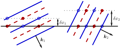
Figure 6: Two source modes, ${\boldsymbol{k}}_{1}$ and ${\boldsymbol{k}}_{2}$, with the same wavenumber $\tilde{k}$. Diagonal lines indicate troughs (solid) and crests (dashed). The observer is towards the bottom. The solid horizontal line indicates the position of the LSS at initial time $\eta$. The dotted horizontal lines indicate the position of the LSS at the first later time that produces perfect anticorrelations with the initial time, so that hot spots (solid circles) line up with cold spots (open circles) and vice versa. Mode ${\boldsymbol{k}}_{1}$, which corresponds to a smaller observed $\ell$, reaches anticorrelation before mode ${\boldsymbol{k}}_{2}$ (since $\delta x_{1}<\delta x_{2}$). A mode ${\boldsymbol{k}}$ parallel to the LSS would never reach anticorrelation, while a mode parallel to the line of sight would correspond to $\ell=0$ (in the flat sky approximation).

IV.1.4 Origin of the difference map power

As we mentioned above, the power spectrum of the difference map, $D_{\ell}^{\eta\eta^{\prime}}$, contains two distinct contributions: the loss of correlations and the change in variance between the two times of observation. To make this explicit, and to determine which contribution is more important, we can use Eqs. (53) and (58) to write

$$D_{\ell}^{\eta\eta^{\prime}} = \left(\sqrt{C_{\ell}(\eta^{\prime})}-\sqrt{C_{\ell}(\eta)}\right)^{2}$$ (78)

$$+\ 2\sqrt{C_{\ell}(\eta)C_{\ell}(\eta^{\prime})}\left(1-\bar{C}_{\ell}^{\eta\eta^{\prime}}\right)$$

$$= C_{\ell}(\eta)\left[\frac{1}{4}\left(\frac{\delta C_{\ell}}{C_{\ell}(\eta)}\right)^{2}+2\left(1-\bar{C}_{\ell}^{\eta\eta^{\prime}}\right)\right]$$

$$+\ {\cal O}\left(\frac{\delta\eta}{\eta_{\rm LS}}\right)^{3}.$$

The first line above is exact, while in the second we have dropped higher order terms in

$$\frac{\delta C_{\ell}}{C_{\ell}(\eta)}\sim\frac{\delta\eta}{\eta_{\rm LS}}$$ (79)

[recall Eq. (34)]. With a calculation similar to that leading to Eq. (67), it is straightforward to show that, for short time intervals ($\delta\eta/\eta_{\rm LS}\ll 1)$, we have $1-\bar{C}_{\ell}^{\eta\eta^{\prime}}\propto(\delta\eta/\eta_{\rm LS})^{2}$, so that the two terms in square brackets in Eq. (78) are of the same order in $\delta\eta/\eta_{\rm LS}$.

The first term in square brackets in the expression (78) is due entirely to the change in variance $\delta C_{\ell}$, while the second term is due solely to the loss of correlations between $a_{\ell m}(\eta)$ and $a_{\ell m}(\eta^{\prime})$ [recall Eq. (57)]. But from Eq. (69) we have

$$D_{\ell}^{\eta\eta^{\prime}}\sim\left(\frac{\delta\eta}{\eta_{\rm LS}}\right)^{2}\ell^{2}C_{\ell}(\eta).$$ (80)

This expression dominates the change in variance contribution to Eq. (78) by a factor $\ell^{2}$. Therefore, for all but the very largest angular scales (smallest $\ell$), the second term in the brackets in (78) must dominate over the first, and so the power spectrum $D_{\ell}^{\eta\eta^{\prime}}$ is dominated by the loss in correlations. This can be confirmed by a direct computation in the flat sky approximation, which gives

$$2C({\boldsymbol{\ell}},\eta)\left(1-\bar{C}^{\eta\eta^{\prime}}\!({\boldsymbol{\ell}})\right)=D^{\eta\eta^{\prime}}\!({\boldsymbol{\ell}}),$$ (81)

at lowest order in $\delta\eta/\eta_{\rm LS}$. This means that the flat sky approximation to $D_{\ell}^{\eta\eta^{\prime}}$ captures only the (dominant) contribution due to loss of correlations. This is not surprizing: because of the scaling relation (29), the flat sky difference map defined in Eq. (62) is closely related to the “normalized” difference map defined in Eq. (56).

One further contribution to the difference map arises if we consider the absolute temperature anisotropies $\delta T$ rather than the relative quantity $\delta T/T$, where $T$ is the mean temperature. Recall from Section III.2 that, if we consider the absolute spectrum $T^{2}C_{\ell}$ instead of the relative quantity $C_{\ell}$, then the difference $\delta(T^{2}C_{\ell})\equiv T^{2}(\eta^{\prime})C_{\ell}(\eta^{\prime})-T^{2}(\eta)C_{\ell}(\eta)$ receives an extra contribution due to the expansion redshift. In that case we showed that the extra contribution is of the same order as the geometrical scaling part [recall Eq. (35)].

We can now repeat this calculation for the difference map power spectrum. The difference map in absolute temperature units is

$$\delta(Ta_{\ell m})=T\left[-\frac{\delta\eta}{(aH)^{-1}}a_{\ell m}+\delta a_{\ell m}\right]$$ (82)

at lowest order in $\delta\eta/(aH)^{-1}$, where we have used $\dot{T}=-HT$. Therefore the corresponding power spectrum becomes

$$\langle\delta(Ta_{\ell m})\delta(Ta_{\ell m})^{\ast}\rangle =T^{2}\left[D_{\ell}^{\eta\eta^{\prime}}+\left(\frac{\delta\eta}{(aH)^{-1}}\right)^{2}C_{\ell}\right.$$ (83)

$$+\frac{\delta\eta}{(aH)^{-1}}\left(D_{\ell}^{\eta\eta^{\prime}}-\delta C_{\ell}\right)\Bigg{]},$$

where we have used the expressions (52), (53), and (55). Next, retaining only terms to lowest order in $\delta\eta/(aH)^{-1}\sim\delta\eta/\eta_{\rm LS}$, and using Eq. (79), we have

$$\langle\delta(Ta_{\ell m})\delta(Ta_{\ell m})^{\ast}\rangle=T^{2}\left[D_{\ell}^{\eta\eta^{\prime}}+{\cal O}\left(\frac{\delta\eta}{\eta_{\rm LS}}\right)^{2}C_{\ell}\right].$$ (84)

But then Eq. (80) tells us that the first term on the right-hand side of Eq. (84) dominates for all but the very largest angular scales [just as we argued above for Eq. (78)], and so

$$\langle\delta(Ta_{\ell m})\delta(Ta_{\ell m})^{\ast}\rangle\simeq T^{2}D_{\ell}^{\eta\eta^{\prime}}.$$ (85)

In other words, the part of the power spectrum for the absolute difference map $\delta(Ta_{\ell m})$ which is due to the expansion redshift is subdominant. Thus, contrary to the case with $\delta C_{\ell}$, it is irrelevant for the difference map whether we consider absolute or relative temperature differences (apart from on the very largest scales).

In hindsight this result could have been anticipated directly from Eq. (82), since we expect that the change $\delta a_{\ell m}$, corresponding to the time interval $\delta\eta$, should be

$$\delta a_{\ell m}\sim\frac{\delta\eta}{\eta_{\rm LS}}\ell a_{\ell m},$$ (86)

so that the first term on the right-hand side of Eq. (82), which is due to the expansion redshift, is subdominant on all but the largest scales. Intuitively, the change in $a_{\ell m}$ due to a change in observation time $\delta\eta$ grows as the wavelength of the source modes decreases (for constant mode amplitude), since the corresponding increase in radius of the LSS is a larger fraction of a shorter wavelength mode. On the other hand, the change in $Ta_{\ell m}$ due to the expansion redshift is independent of scale $\ell$.

Similarly, the contribution to the difference map due to loss of correlations, which is described crudely by Eq. (86), is expected to dominate over the contribution due to changing variance $C_{\ell}$, which is roughly independent of $\ell$, as we showed rigorously above.

IV.2 Time evolution from CAMB

IV.2.1 Power spectrum and correlation function

We have computed the correlation function $C_{\ell}^{\eta\eta^{\prime}}$ from Eq. (54) and the difference map power spectrum $D_{\ell}^{\eta\eta^{\prime}}$ from Eq. (53) numerically using our modified version of camb to extract $T(k,\ell,r_{\rm LS})$ at different $r_{\rm LS}$ (as outlined in Section III.6), using the cosmological parameters of our fiducial $\Lambda$CDM model. In Fig. 7 we display $D_{\ell}^{\eta\eta^{\prime}}$ for the times $\eta$ and $\eta^{\prime}$ corresponding to today, $a_{\rm obs}=1$, and future times when $a^{\prime}_{\rm obs}=1+\delta a$, for the cases $\delta a=10^{-4}$, $0.001$, $0.01$, and $0.1$. For small increments $\delta a$ these curves exhibit precisely the quadratic scaling $D_{\ell}^{\eta\eta^{\prime}}\propto(\delta\eta)^{2}$ that we predicted in Eq. (59), and the slope of $D_{\ell}^{\eta\eta^{\prime}}$ for small $\ell$ matches our analytical prediction for the Sachs-Wolfe plateau, Eq. (74). For large increments $\delta a$ the difference map power spectrum approaches the sum of the individual power spectra as the correlation function decays to zero, as we expect according to Eq. (53). Generally, these curves exhibit the heavily blue-tilted form we predicted in the previous subsection, due to the more rapid loss of correlations on smaller angular scales.

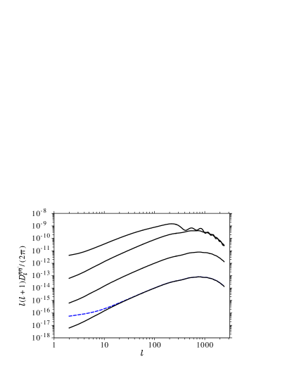
Figure 7: Difference map angular power spectrum $D_{\ell}^{\eta\eta^{\prime}}$ calculated from our modified version of camb (solid lines) for the two times corresponding to $a_{\rm obs}=1$ and $a^{\prime}_{\rm obs}=1+\delta a$, for the cases (top to bottom) $\delta a=0.1$, $0.01$, $0.001$, and $10^{-4}$. Also shown is the analytical result (dashed curve) calculated using Eq. (69) for $\delta a=10^{-4}$.

Also shown in Fig. 7 is the curve calculated from the flat-sky analytical expression, Eq. (69), for the case $\delta a=10^{-4}$. This curve coincides extremely well with the numerical result for $\ell\gtrsim 20$. The departures at large scales are due to two factors. First, the flat sky approximation is poor at those scales. Second, Eq. (69) was derived under the assumption that all anisotropies were primary, which is not the case for the ISW contribution.

In Fig. 8 we plot the normalized correlation function $\bar{C}_{\ell}^{\eta\eta^{\prime}}$, calculated using our modified version of camb for our fiducial $\Lambda$CDM model, between the set of $a_{\ell m}$s observed at $\eta$ and $\eta^{\prime}$. Here, $\eta$ corresponds to an observation of the CMB sky today at $a_{\rm obs}=1$ and $\eta^{\prime}$ to an observation at $a^{\prime}_{\rm obs}=1+\delta a$, where we illustrate the cases $\delta a=0.001$, $0.01$, $0.03$ and $0.1$. For the smallest interval $\delta a$, we find very strong correlation between the two sky maps, as expected. The correlations fall off as $\delta a$ increases, with the sky maps becoming somewhat anticorrelated for intermediate intervals before $\bar{C}_{\ell}^{\eta\eta^{\prime}}$ decays to zero at the largest intervals.

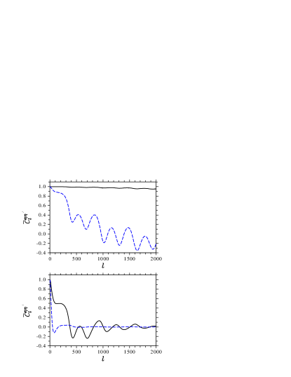
Figure 8: Normalized correlation function $\bar{C}_{\ell}^{\eta\eta^{\prime}}$ between the CMB sky observed today ($a=1$) and at $a=1+\delta a$, calculated with our modified version of camb, for $\delta a=0.001$ (top panel, solid curve), $0.01$ (top panel, dashed curve), $0.03$ (bottom panel, solid), and $0.1$ (bottom panel, dashed). Anticorrelations are seen to develop as $\delta a$ increases, before the correlation function decays to zero for large $\delta a$.

The general features of the correlation function can be understood by considering the detailed arguments presented in the previous subsection. For $\delta a\ll 1$ the increase in the LSS radius corresponding to the interval $\delta a$ is $\delta r_{\rm LS}=H_{0}^{-1}\delta a$. For the case of $\delta a=0.01$, using $H_{0}=73$ ${\rm km}\,{\rm s}^{-1}{\rm Mpc}^{-1}$, we find $\delta r_{\rm LS}=40.9$ Mpc, corresponding to a comoving wavenumber $k=0.15$ ${\rm Mpc^{-1}}$. This wavenumber is much larger than the wavenumber of the first acoustic peak, given by $k=\pi/s_{\rm LS}=0.021$ ${\rm Mpc^{-1}}$, where $s_{\rm LS}\simeq 150$ Mpc is the sound horizon at last scattering. Hence, for this $\delta a$, we are essentially sampling the same set of inhomogeneities which give rise to the first acoustic peak at both times, and so we expect fluctuations to be correlated on these scales. Indeed, we see from Fig. 8 for $\delta a=0.01$ that $\bar{C}_{\ell}^{\eta\eta^{\prime}}\simeq 0.9$ for the first acoustic peak scale, $\ell\simeq 220$. Extending this argument, we expect that $\bar{C}_{\ell}^{\eta\eta^{\prime}}\rightarrow 1$ as $\ell\rightarrow 0$ for fixed $\delta a$, as the largest scale (smallest $k$) features should be most correlated, and of course we similarly expect $\bar{C}_{\ell}^{\eta\eta^{\prime}}\rightarrow 1$ as $\delta a\rightarrow 0$ for fixed $\ell$.

The presence of anticorrelations was discussed in Section IV.1, where we derived the behaviour of the correlation function in the flat sky approximation for the case of a delta-source at wavenumber $k=\tilde{k}$. The result, Eq. (75), exhibited oscillating positive and negative correlations, with the first anticorrelations occuring earlier for smaller scales (larger $\tilde{k}$), as we have confirmed here for a realistic spectrum using camb. Eq. (75) also described anticorrelations occuring earlier for smaller $\ell$, with $\tilde{k}$ fixed. This behaviour is not visible in the actual correlation function plotted in Fig. 8, since the real primordial power spectrum is far from being a delta-source. If we consider a small subset of $k$ modes, e.g. those corresponding to the fourth acoustic peak scale, then some of those modes will be aligned nearly parallel to our line of sight and hence produce early anticorrelations at small $\ell$ for some $\delta a$ (recall Fig. 6). However, there are many more modes due to power at smaller $k$ that are still tightly correlated at the same $\delta a$ and hence result in $\bar{C}_{\ell}^{\eta\eta^{\prime}}\simeq 1$ for small $\ell$.

IV.2.2 Sky maps

Assuming Gaussianity, generating a single realization of a set of $a_{\ell m}$s usually involves drawing each $a_{\ell m}(\eta)$ independently from a Gaussian distribution with variance $C_{\ell}(\eta)$. With the correlation function $C_{\ell}^{\eta\eta^{\prime}}$, we have a measure of the degree of correlation between $a_{\ell m}$s at two different times. Hence, given a set of $a_{\ell m}$s at the first time, the variance of the distribution at each time, and the correlation between them, one can generate a realization of a second set of $a_{\ell m}$s at some later time.

Formally, we draw the new set of $a_{\ell m}$s from the likelihood function

$$P(X_{i})=\frac{1}{2\pi|C|^{1/2}}\exp\left(-\frac{1}{2}X_{i}^{T}C^{-1}X_{i}\right)\,,$$ (87)

with

$$C=\left(\begin{matrix}C_{\ell}^{\eta\eta}&C_{\ell}^{\eta\eta^{\prime}}\cr C_{\ell}^{\eta\eta^{\prime}}&C_{\ell}^{\eta^{\prime}\eta^{\prime}}\end{matrix}\right)\,,$$ (88)

where $X_{i}$ is a random 2-vector containing each $a_{\ell m}$ coefficient at $\eta$ and $\eta^{\prime}$, and we have relabeled the variance of the $a_{\ell m}(\eta)$ distribution at each time by $C_{\ell}^{\eta\eta}$ and $C_{\ell}^{\eta^{\prime}\eta^{\prime}}$.

We illustrate the likelihood function in Fig. 9 for the $a_{2m}$ and $a_{5m}$ modes, where $\eta$ corresponds to an observation at $a_{\rm obs}=1$ and $\eta^{\prime}$ to $a_{\rm obs}=2.0$. The $a_{2m}$ coefficients are more tightly correlated than their $a_{5m}$ counterparts, since for such a large $\delta a$ the correlation rapidly falls off as $\ell$ increases. It is also noticeable that the contours of the likelihood are slightly elongated vertically, due to the increased variance of $a_{\ell m}(\eta^{\prime})$ on large scales resulting from the increasing ISW effect.

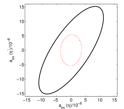
Figure 9: Distribution from which the $a_{\ell m}$s are drawn. Here, $\eta$ corresponds to $a_{\rm obs}=1$ and $\eta^{\prime}$ to $a_{\rm obs}=2.0$, and contours show the $2\sigma$ error ellipse. The distribution of $a_{2m}$ is shown by the solid contour, which has a correlated set of variances $C_{2}(\eta)$ and $C_{2}(\eta^{\prime})$. The distribution of $a_{5m}$, shown by the dotted contour, has a smaller variance at both times and these are much less correlated.

Therefore, our method of generating CMB sky maps involves firstly generating a random realization at some initial time, and then generating all subsequent realizations by mapping the $a_{\ell m}$s using the correlation function. For large $\delta a$, where the $a_{\ell m}$s are uncorrelated, we are essentially selecting a completely new set of coefficients. For small $\delta a$, $\bar{C}_{\ell}^{\eta\eta^{\prime}}$ approaches unity and the $a_{\ell m}$s map trivially according to $a_{\ell m}(\eta)\rightarrow a_{\ell m}(\eta^{\prime})$. At some intermediate intervals, anticorrelation favours a reversal of sign of the $a_{\ell m}$s, i.e. hot spots are mapped to cold spots and vice versa.

We generate maps using the HEALPix code with $n_{\rm side}=512$, corresponding to a pixel resolution of $6.87$ arcmin. We present a series of these maps in Fig. 10, plotting the fractional temperature fluctuation $\delta T_{i}/T$ at each pixel $i$. For presentational clarity we show a patch of sky covering $\sim 1000$ square degrees, and use modes up to $\ell_{\rm max}=1000$. We generate the first map at $a_{\rm obs}=1$, and show subsequent maps at $a_{\rm obs}=1+\delta a$, where $\delta a=0.001$, $0.01$, $0.1$, and $1.0$. We also show the difference map for each observation relative to $a_{\rm obs}=1$. We have checked that the power spectra reconstructed from our simulated sky maps agree with the intended spectra to within sample variance. Note that for the sky maps in Fig. 10 we did not use the actual WMAP data for the present time; rather, we simply generated a random initial map according to the required $C_{\ell}$ spectrum.

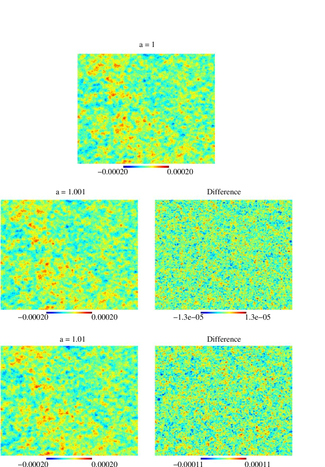
Figure 10: Simulated map realizations (top and left panels) and difference map (relative to $a_{\rm obs}=1$) (right panels) for $\delta a=10^{-3}$ (middle panels, corresponding to a $13$ Myr interval) and $10^{-2}$ (bottom panels, $130$ Myr). Note the vastly different power scales between the sky and difference maps. The maps presented here are for a patch of sky covering $\sim 1000$ square degrees. High resolution version available at http://www.astro.ubc.ca/people/scott/future.html.

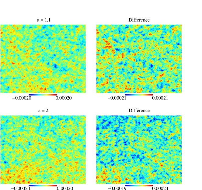
Figure 10: (Continued.) Simulated map realizations (left panels) and difference (right) for $\delta a=0.1$ (top) and $1.0$ (bottom). High resolution version available at http://www.astro.ubc.ca/people/scott/future.html.

Visually, the $\delta a=0.001$ map is extremely similar to the initial map. The variance of the map, given by

$$\left\langle\left(\frac{\delta T}{T}\right)^{2}\right\rangle_{\rm map}=\frac{1}{N_{\rm pix}}\sum_{i}^{N_{\rm pix}}\left(\frac{\delta T_{i}}{T}\right)^{2}\,,$$ (89)

is over four orders of magnitude higher than the difference map variance. For $\delta a=0.01$, the primary temperature fluctuations have a variance around two orders of magnitude more than the difference map, and changes in small scale structure (from the initial map) are clearly apparent.

For $\delta a=0.1$ and $1.0$, the variance of the difference is actually larger then the temperature fluctuations at that time, and acoustic scale structures are visible in the difference. This is understandable from our discussion of the correlation function—at these times the correlation on all but the very largest scales has dropped to zero, so that the variance of the difference approaches the sum of the initial and final map variances [recall Eq. (53)].

Finally, in Fig. 11 we present a simulated sky map for the asymptotic future. This map clearly differs from today’s map, with the dramatic increase in large scale power due to the ISW effect readily apparent. For this map, we derived the initial $a_{\ell m}$ coefficients up to $\ell=20$ from the WMAP Internal Linear Combination map Hinshaw et al. (2007) (for $\ell>20$ we generated random initial modes instead of using the real data, since the normalized correlation is negligible on those scales at these very late times).

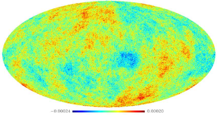
Figure 11: Simulated map realization for the asymptotic future. High resolution version available at http://www.astro.ubc.ca/people/scott/future.html.

High resolution versions of these sky maps, together with animations illustrating the evolution of the CMB sky maps, $C_{\ell}$ spectra, and correlation functions, are available at http://www.astro.ubc.ca/people/scott/future.html.

V Discussion

We have systematically described the temporal evolution of the CMB, beginning with the mean temperature and dipole, and then moving to the anisotropy power spectrum. We found that the evolution of the spectrum is described at all but the largest angular scales by a simple scaling relation. At large scales the ISW contribution grows to dominate even the first acoustic peak at late times. The extra optical depth due to reionization is negligible into the future.

We have introduced a correlation function between the CMB sky maps at different times which quantitatively encodes the intuitive notion that for small enough observation time intervals $\delta\eta$ and for source modes with small enough wavenumber $k$, the anisotropies observed at the two times should be very similar. Closely related is the power spectrum of the difference map $D_{\ell}^{\eta\eta^{\prime}}$. We showed that the difference $\delta C_{\ell}$ scales like $\delta\eta$ for small intervals, while $D_{\ell}^{\eta\eta^{\prime}}$ scales like $(\delta\eta)^{2}$. The sensitivity of $D_{\ell}^{\eta\eta^{\prime}}$ to changes in the sky maps is dominated by the loss of correlations at small angular scales, and the contributions from the change in variance $C_{\ell}$, as well as the change due to expansion redshift (if we consider absolute quantities) are subdominant. All of our numerical results were independently confirmed analytically, and the validity of the necessary analytical approximations was elucidated by the numerics.

The quantities we described in this work will be crucial to answering the question of the experimental detectability of a change in the CMB, or, more precisely, the question “how long must we wait to be able to confidently observe a change?” While the different time interval scalings we found for $\delta C_{\ell}$ and $D_{\ell}^{\eta\eta^{\prime}}$ might suggest that attempting to measure $\delta C_{\ell}$ would be much more favourable for small $\delta\eta$, the situation is more subtle. In a separate paper Moss et al. (2007) we quantify the detectability of changes in the CMB.

On sufficiently long time scales the CMB evolution we have described will be obvious, and hence it is natural to ask what cosmological information a measurement of such changes might eventually provide to future cosmologists. A measurement of the cooling rate of the mean temperature $T$ would provide an independent and novel determination of the local Hubble rate $H_{0}$, through the relation $\dot{T}=-HT$. As far as the primary temperature anisotropies are concerned, according to Eq. (69) the shape of the difference map spectrum $D_{\ell}^{\eta\eta^{\prime}}$ is determined by the $C_{\ell}$ spectrum [and the primordial spectrum through the quantity $C^{(n_{S}+2)}({\boldsymbol{\ell}},\eta)$], so a measurement of the shape of $D_{\ell}^{\eta\eta^{\prime}}$ should not provide much new information. With our assumption of a spatially flat geometry, the amplitude of $D_{\ell}^{\eta\eta^{\prime}}$ is determined by the ratio $\delta x_{\rm LS}/x_{\rm LS}=\delta t/(a_{0}x_{\rm LS})$. Thus a measurement of the amplitude would directly fix the LSS radius $x_{\rm LS}$ and hence provide an independent constraint on the parameters $\Omega_{m}$, $\Omega_{\Lambda}$, and $H_{0}$. (This determination of $x_{\rm LS}$ is replaced by a determination of the angular diameter distance for spatially curved models.) The radius of the LSS is currently fixed, through observations of the accoustic angular scale, only up to the uncertainty in the matter content at last scattering. At very late times much additional information will of course become available as new modes become visible on the growing LSS.

We have focussed entirely on primordial anisotropies here. There are additional issues which arise when one considers secondary anisotropies, like gravitational lensing and Sunyaev-Zel’dovich effects, as well as time-dependent foregrounds of course. Such considerations depend much more heavily on the less well understood non-linear scales of structure, and so we leave this for others to pursue. We expect that there is plenty of time to pursue these ideas before any of these variations would be detectable.

When this work was nearly complete, a related study appeared by Lange and Page Lange and Page (2007). Those authors calculated future $C_{\ell}$ spectra using camb. They also defined a correlation fuction equivalent to our Eq. (54), calculated it using camb, and generated simulated future sky maps. While they made no attempt at an analytical description of the evolution, their numerical results appear to agree with ours where they overlap. Furthermore, they made an estimate of the observability of the CMB evolution, which we have deferred to Ref. Moss et al. (2007).

*

Appendix A The flat sky approximation

The Bessel functions appearing in the various expressions relating primordial fluctuations to observed CMB anisotropies severely limit the extent to which analytical results can be obtained. However, a simple approximation scheme, based on treating a small patch of the sky (and hence of the spherical LSS) as flat, allows us to use ordinary plane wave expansions and thereby to do “CMB without Bessel functions”. This small-angle approximation is expected to be accurate up to terms of order $1/\ell$, so that it is entirely appropriate for describing the acoustic peak structure of the CMB.

The flat sky approximation begins (see, e.g., Liddle and Lyth (2000)) by replacing Eq. (12) relating the observed temperature anisotropies with the perturbation functions on the LSS, $\phi_{i}$, in the strong coupling/free streaming approximation, by

$$\frac{\delta T(\boldsymbol{\theta},\eta)}{T(\eta)}=F(\phi_{i}(x_{\rm LS},x_{\rm LS}\boldsymbol{\theta},\eta_{\rm LS})).$$ (90)

Here $\boldsymbol{\theta}$ is a $2$-dimensional vector whose components represent the angular displacement in two orthogonal directions from the centre of the small patch of sky. In the Cartesian comoving coordinate vector $(x_{\rm LS},x_{\rm LS}\boldsymbol{\theta})$, the first component is parallel to, and the second two orthogonal to, the line of sight to the centre of the patch. The coordinate value $x_{\rm LS}=\eta-\eta_{\rm LS}$ refers to the comoving distance to the LSS from the point of observation. Analogously to Eq. (13) we can write

$$F(\phi_{i}(x_{\rm LS},x_{\rm LS}\boldsymbol{\theta},\eta_{\rm LS}))=\phi_{1}(x_{\rm LS},x_{\rm LS}\boldsymbol{\theta},\eta_{\rm LS})+\frac{\partial}{\partial x_{\rm LS}}\phi_{2}(x_{\rm LS},x_{\rm LS}\boldsymbol{\theta},\eta_{\rm LS})$$ (91)

for the monopole and dipole contributions. In place of the spherical harmonic expansion for the temperature fluctuation, Eq. (15), we here use a $2$-dimensional Fourier expansion in terms of the continuous vector ${\boldsymbol{\ell}}$ which replaces $\ell$ and $m$:

$$\frac{\delta T(\boldsymbol{\theta},\eta)}{T(\eta)}=\frac{1}{2\pi}\int d^{2}{\boldsymbol{\ell}}\,a({\boldsymbol{\ell}})e^{i\boldsymbol{\theta}\cdot{\boldsymbol{\ell}}}.$$ (92)

The statistical properties of the coefficients $a({\boldsymbol{\ell}})$ can be determined in a manner completely analogous to that used for the spherical case in Section III.1. Fourier expanding the perturbations $\phi_{i}$ according to

$$\phi_{i}(x_{\rm LS},x_{\rm LS}\boldsymbol{\theta})=\frac{1}{(2\pi)^{3/2}}\int d^{2}{\boldsymbol{k_{\perp}}}dk_{x}\,\phi_{i}({\boldsymbol{k}})e^{i{\boldsymbol{k_{\perp}}}\cdot x_{\rm LS}\boldsymbol{\theta}}e^{ik_{x}x_{\rm LS}},$$ (93)

where $k_{x}$ and ${\boldsymbol{k_{\perp}}}$ are Cartesian components of the wavevector ${\boldsymbol{k}}$ parallel and orthogonal to the line of sight, respectively, allows us to identify

$${\boldsymbol{\ell}}=x_{\rm LS}{\boldsymbol{k_{\perp}}}.$$ (94)

This tells us that ${\boldsymbol{\ell}}$, the flat sky approximation to the spherical indices $\ell$ and $m$, is directly proportional to the component of the LSS fluctuation wavevector orthogonal to the line of sight, and that the relationship scales with the conformal time (or comoving distance) to the LSS, exactly as expected. Since ${\boldsymbol{k_{\perp}}}$ is only a component of the wavevector ${\boldsymbol{k}}$, Eq. (94) encodes the familiar fact that the mapping from $k$ to $\ell$ is not one-to-one—rather, a range of $k$’s is mapped to a particular $\ell$ value.

Using these expressions, we find

$$a({\boldsymbol{\ell}},\eta)=\frac{1}{\sqrt{2\pi}x_{\rm LS}^{2}}\int_{-\infty}^{\infty}dk_{x}{\cal R}(k_{x},{\boldsymbol{\ell}}/x_{\rm LS})T_{\rm FS}(k,k_{x})e^{ik_{x}x_{\rm LS}},$$ (95)

where the flat sky transfer function is

$$T_{\rm FS}(k,k_{x})\equiv A_{1}(k)+ik_{x}A_{2}(k),$$ (96)

and the $A_{i}$ are again defined by Eq. (11). Finally, using the statistical properties of ${\cal R}$ encoded in Eq. (10), the equal-time correlation function of $a({\boldsymbol{\ell}})$ becomes

$$\langle a({\boldsymbol{\ell}},\eta)a^{\ast}({\boldsymbol{\ell}}\,^{\prime},\eta)\rangle=C({\boldsymbol{\ell}},\eta)\delta^{2}({\boldsymbol{\ell}}-{\boldsymbol{\ell}}\,^{\prime}),$$ (97)

where

$$C({\boldsymbol{\ell}},\eta)\equiv\frac{\pi}{x_{\rm LS}^{2}}\int_{-\infty}^{\infty}dk_{x}\frac{{\cal P_{\cal R}}(k)|T(k,k_{x})|^{2}}{(k_{x}^{2}+{\boldsymbol{k_{\perp}}}^{2})^{3/2}}.$$ (98)

Again, we find that the coefficients $a({\boldsymbol{\ell}})$ for different ${\boldsymbol{\ell}}$ modes are uncorrelated.

Notice that the time dependence of $C({\boldsymbol{\ell}},\eta)$ is carried in the prefactor $1/x_{\rm LS}^{2}$ as well as in the terms containing ${\boldsymbol{k_{\perp}}}$ through Eq. (94) (if ${\boldsymbol{\ell}}$ is held constant), whereas in the spherical case, Eq. (24), the Bessel functions carry the time dependence. Also, the complete absence of oscillatory functions in Eq. (98) means that it will be much easier to evaluate the CMB spectrum in the flat sky approximation than in the spherical case, both analytically and numerically.

In particular, we can easily apply Eq. (98) to rederive the scaling relation Eq. (29). Eq. (94) tells us that ${\boldsymbol{k_{\perp}}}$ is invariant under the transformation $x_{\rm LS}\rightarrow x_{\rm LS}^{\prime}$ and ${\boldsymbol{\ell}}\rightarrow{\boldsymbol{\ell}}\,^{\prime}={\boldsymbol{\ell}}x_{\rm LS}^{\prime}/x_{\rm LS}$. Therefore, Eq. (98) immediately implies that

$$\ell^{\prime 2}C({\boldsymbol{\ell}}\,^{\prime},\eta^{\prime})=\ell^{2}C({\boldsymbol{\ell}},\eta),$$ (99)

where $\ell\equiv|{\boldsymbol{\ell}}|$, regardless of the form of the transfer functions $A_{i}(k)$ or of the primordial power spectrum ${\cal P_{\cal R}}(k)$.

References

- Scott and Smoot (2006) D. Scott and G. F. Smoot, in W.-M. Yao et al., J. Phys. G 33, 1 (2006).
- Challinor (2004) A. Challinor (2004), eprint astro-ph/0403344.
- Hu and Dodelson (2002) W. Hu and S. Dodelson, Ann. Rev. Astron. Astrophys. 40, 171 (2002), eprint astro-ph/0110414.
- Spergel et al. (2007) D. N. Spergel et al. (WMAP), Astrophys. J. Suppl. 170, 377 (2007), eprint astro-ph/0603449.
- Spergel et al. (2003) D. N. Spergel et al. (WMAP), Astrophys. J. Suppl. 148, 175 (2003), eprint astro-ph/0302209.
- Fixsen et al. (1996) D. J. Fixsen et al., Astrophys. J. 473, 576 (1996), eprint astro-ph/9605054.
- Mather et al. (1999) J. C. Mather, D. J. Fixsen, R. A. Shafer, C. Mosier, and D. T. Wilkinson, Astrophys. J. 512, 511 (1999), eprint astro-ph/9810373.
- Lewis et al. (2000) A. Lewis, A. Challinor, and A. Lasenby, Astrophys. J. 538, 473 (2000), eprint astro-ph/9911177.
- Seljak and Zaldarriaga (1996) U. Seljak and M. Zaldarriaga, Astrophys. J. 469, 437 (1996), eprint astro-ph/9603033.
- Gott (1996) J. R. Gott, III, in Clusters, Lensing, and the Future of the Universe, edited by V. Trimble and A. Reisenegger (Astronomical Society of the Pacific, San Francisco, 1996), vol. 88 of Astronomical Society of the Pacific Conference Series, pp. 140–151.
- Loeb (2002) A. Loeb, Phys. Rev. D65, 047301 (2002), eprint astro-ph/0107568.
- Krauss and Scherrer (2007) L. M. Krauss and R. J. Scherrer (2007), eprint arXiv:0704.0221 [astro-ph].
- Caldwell et al. (2003) R. R. Caldwell, M. Kamionkowski, and N. N. Weinberg, Phys. Rev. Lett. 91, 071301 (2003), eprint astro-ph/0302506.
- Moss et al. (2007) A. Moss, J. P. Zibin, and D. Scott (2007), eprint arXiv:0709.4040 [astro-ph].
- Gibbons and Hawking (1977) G. W. Gibbons and S. W. Hawking, Phys. Rev. D15, 2738 (1977).
- Busha et al. (2003) M. T. Busha, F. C. Adams, R. H. Wechsler, and A. E. Evrard, Astrophys. J. 596, 713 (2003), eprint astro-ph/0305211.
- Hinshaw et al. (2007) G. Hinshaw et al. (WMAP), Astrophys. J. Suppl. 170, 288 (2007), eprint astro-ph/0603451.
- Kogut et al. (1993) A. Kogut et al., Astrophys. J. 419, 1 (1993), eprint astro-ph/9312056.
- Tully et al. (2007) R. B. Tully et al. (2007), eprint arXiv:0705.4139 [astro-ph].
- Ma et al. (1998) C. Ma, E. F. Arias, T. M. Eubanks, A. L. Fey, A.-M. Gontier, C. S. Jacobs, O. J. Sovers, B. A. Archinal, and P. Charlot, Astron. J. 116, 516 (1998).
- Hu and Sugiyama (1995) W. Hu and N. Sugiyama, Phys. Rev. D51, 2599 (1995), eprint astro-ph/9411008.
- Dodelson (2003) S. Dodelson, Modern Cosmology (Academic Press, Amsterdam, 2003).
- Sachs and Wolfe (1967) R. K. Sachs and A. M. Wolfe, Astrophys. J. 147, 73 (1967).
- Liddle and Lyth (2000) A. R. Liddle and D. H. Lyth, Cosmological Inflation and Large-Scale Structure (Cambridge University Press, Cambridge, 2000).
- Abramowitz and Stegun (1972) M. Abramowitz and I. A. Stegun, eds., Handbook of Mathematical Functions with Formulas, Graphs, and Mathematical Tables (U.S. Department of Commerce, Washington, D.C., 1972).
- Bond and Efstathiou (1987) J. R. Bond and G. Efstathiou, Mon. Not. Roy. Astron. Soc. 226, 655 (1987).
- Bond et al. (1997) J. R. Bond, G. Efstathiou, and M. Tegmark, Mon. Not. Roy. Astron. Soc. 291, L33 (1997), eprint astro-ph/9702100.
- Zaldarriaga et al. (1997) M. Zaldarriaga, D. N. Spergel, and U. Seljak, Astrophys. J. 488, 1 (1997), eprint astro-ph/9702157.
- Efstathiou and Bond (1999) G. Efstathiou and J. R. Bond, Mon. Not. Roy. Astron. Soc. 304, 75 (1999), eprint astro-ph/9807103.
- Kofman and Starobinsky (1985) L. Kofman and A. A. Starobinsky, Sov. Astron. Lett. 11, 271 (1985).
- Mukhanov et al. (1992) V. F. Mukhanov, H. A. Feldman, and R. H. Brandenberger, Phys. Rept. 215, 203 (1992).
- Kamionkowski and Spergel (1994) M. Kamionkowski and D. N. Spergel, Astrophys. J. 432, 7 (1994), eprint astro-ph/9312017.
- Starobinsky (1985) A. A. Starobinsky, Sov. Astron. Lett. 11, 133 (1985).
- Turner et al. (1993) M. S. Turner, M. J. White, and J. E. Lidsey, Phys. Rev. D48, 4613 (1993), eprint astro-ph/9306029.
- Griffiths et al. (1999) L. M. Griffiths, D. Barbosa, and A. R. Liddle, Mon. Not. Roy. Astron. Soc. 308, 854 (1999), eprint astro-ph/9812125.
- Lange and Page (2007) S. Lange and L. Page (2007), eprint arXiv:0706.3908 [astro-ph].
- Górski et al. (2005) K. M. Górski, E. Hivon, A. J. Banday, B. D. Wandelt, F. K. Hansen, M. Reinecke, and M. Bartelmann, Astrophys. J. 622, 759 (2005), eprint arXiv:astro-ph/0409513.