The Spatial Structure of An Accretion Disk

Abstract

Based on the microlensing variability of the two-image gravitational lens HE 1104–1805 observed between $0.4$ and $8~{}\mu$m, we have measured the size and wavelength-dependent structure of the quasar accretion disk. Modeled as a power law in temperature, $T\propto R^{-\beta}$, we measure a B-band ($0.13~{}\mu$m in the rest frame) half-light radius of $R_{1/2,\rm B}=6.7^{+6.2}_{-3.2}\times 10^{15}~{}$ cm ($68\%$ CL) and a logarithmic slope of $\beta=0.61^{+0.21}_{-0.17}$ ($68\%$ CL) for our standard model with a logarithmic prior on the disk size. Both the scale and the slope are consistent with simple thin disk models where $\beta=3/4$ and $R_{1/2,\rm B}=5.9\times 10^{15}~{}\rm cm$ for a Shakura-Sunyaev disk radiating at the Eddington limit with $10\%$ efficiency. The observed fluxes favor a slightly shallower slope, $\beta=0.55^{+0.03}_{-0.02}$, and a significantly smaller size for $\beta=3/4$.

1. Introduction

A simple theoretical prediction for thermally radiating thin accretion disks well outside the inner disk edge is that the temperature diminishes with radius as $T\propto R^{-3/4}$ (Shakura & Sunyaev, 1973). This implies a characteristic size at wavelength $\lambda$ of $R_{\lambda}\propto\lambda^{4/3}$, where $R_{\lambda}$ is the radius at which $kT=hc/\lambda$. Needless to say, it is unlikely that disks are this simple (e.g. Blaes, 2004), but measurement of the size-wavelength scaling would be a fundamental test for any disk theory. While the angular sizes of quasar accretion disks are far too small to be resolved by direct observation, gravitational lenses can serve as natural telescopes to probe accretion disk structure on these scales.

Here we make the first such measurement of this size-wavelength scaling. Our approach, gravitational microlensing of a quasar, will be unfamiliar to the AGN community, but it is the only method with the necessary spatial resolution available to us for the foreseeable future (see the review by Wambsganss, 2006). The stars in the lens galaxy near the image of a multiply-imaged quasar generate complex caustic networks with a characteristic scale called the Einstein radius $R_{\rm E}$ set by the mean stellar mass $\left<M\right>$. For the lens system we consider here, HE 1104–1805, $\left<R_{\rm E}\right>=3.6\times 10^{16}(\left<M\right>/hM_{\sun})^{1/2}~{}\rm cm$. Because the magnification diverges on the caustic curves of the pattern and the source is moving relative to the lens and observer, microlensing allows us to study the spatial structure of anything smaller than $\left<R_{\rm E}\right>$. Using microlensing to probe scales smaller than $R_{\rm E}$ has been successfully applied to resolve stars in Galactic microlensing events (e.g. Albrow et al., 2001). For quasars, this has been considered analytically or with simulations (e.g. Agol & Krolik, 1999; Goicoechea et al., 2004; Grieger, Kayser & Schramm, 1991), but the data and algorithms needed to implement the programs have only become available recently (see Kochanek, 2004).

HE 1104–1805 is a doubly imaged radio-quiet quasar at $z_{s}=2.319$ with a separation of $3\farcs 15$ (Wisotzki et al., 1993). The lens at $z_{l}=0.729$ was discovered in the near-IR by Courbin, Lidman & Magain (1998) and with HST (Remy et al., 1998; Lehár et al., 2000). Here we analyze 13 years of photometric data in 11 bands from the mid-IR to B-band using the methods of Kochanek (2004) to measure the wavelength-dependent structure of this quasar modeled as a power law $R_{\lambda}\propto\lambda^{1/\beta}$. We assume a flat $\Lambda$CDM cosmological model with $\Omega_{M}=0.3$ and $H_{0}=70~{}\rm km~{}s^{-1}~{}Mpc^{-1}$ and report the disk sizes assuming a mean inclination of $\cos{i}=1/2$. In §2 we describe the data set and our methods, and §3 presents our measurement results and our conclusions.

2. Data and Methods

We included observations of HE 1104–1805 in 11 bands: B, V, R, I, J, H, K, $3.6~{}\mu{\rm m}$, $4.5~{}\mu{\rm m}$, $5.8~{}\mu{\rm m}$, and $8.0~{}\mu{\rm m}$. These included our own SMARTS optical/near-IR, SOAR near-IR, HST and Spitzer IRAC data (Poindexter et al., 2007), R-band monitoring data by Ofek & Maoz (2003), the V-band monitoring data from Schechter et al. (2003) and Wyrzykowski et al. (2003), and earlier data from Remy et al. (1998), Gil-Merino, Wisotzki & Wambsganss (2002), Courbin et al. (1998), and Lehár et al. (2000). Where possible we corrected the light curves for the 152 day time delay between the images we measured in Poindexter et al. (2007). Where we could not, we broadened the photometric uncertainties by 0.07 mag so that the flux ratio uncertainties would be larger by the 0.1 mag shifts we found between time-delay corrected and uncorrected flux ratios. The light curve is plotted along with one of the light curve models from our analysis in Figure 1. As pointed out in Poindexter et al. (2007), image A has slowly switched from being bluer than image B to being redder in the optical/near-infrared (see Figure 1), while the mid-infrared flux agrees with the flux ratio of the broad emission lines (Wisotzki et al., 1993).

Determining the structure of the disk as a function of wavelength from such data is relatively straight forward. The divergences on the caustics of the microlensing magnification patterns are only renormalized by the finite size of the source quasar because the observed magnification is the convolution of the pattern with the source structure. Thus, larger emission regions will show smaller variability amplitudes than smaller emission regions because they smooth the patterns more. As we go from the K-band to the B-band, the radius of a standard thin disk with $R_{\lambda}\propto\lambda^{4/3}$, changes by a factor of $8.6$, corresponding to a change in the disk area of almost two orders of magnitude. We see in Fig. 1 that the bluer wavelengths show larger amplitudes than the red wavelengths, so we immediately know that the blue emission regions are more compact than the red.

Our analysis uses the Bayesian Monte Carlo method of Kochanek (2004) to analyze the data. In essence, we randomly draw large numbers of trial light curves from a range of physical models, fit them to the data and then use Bayesian statistics to derive probability distributions for the disk structure. We need, however, to discuss the physical variables used in the models over which we average as well as our model for the structure of the accretion disk.

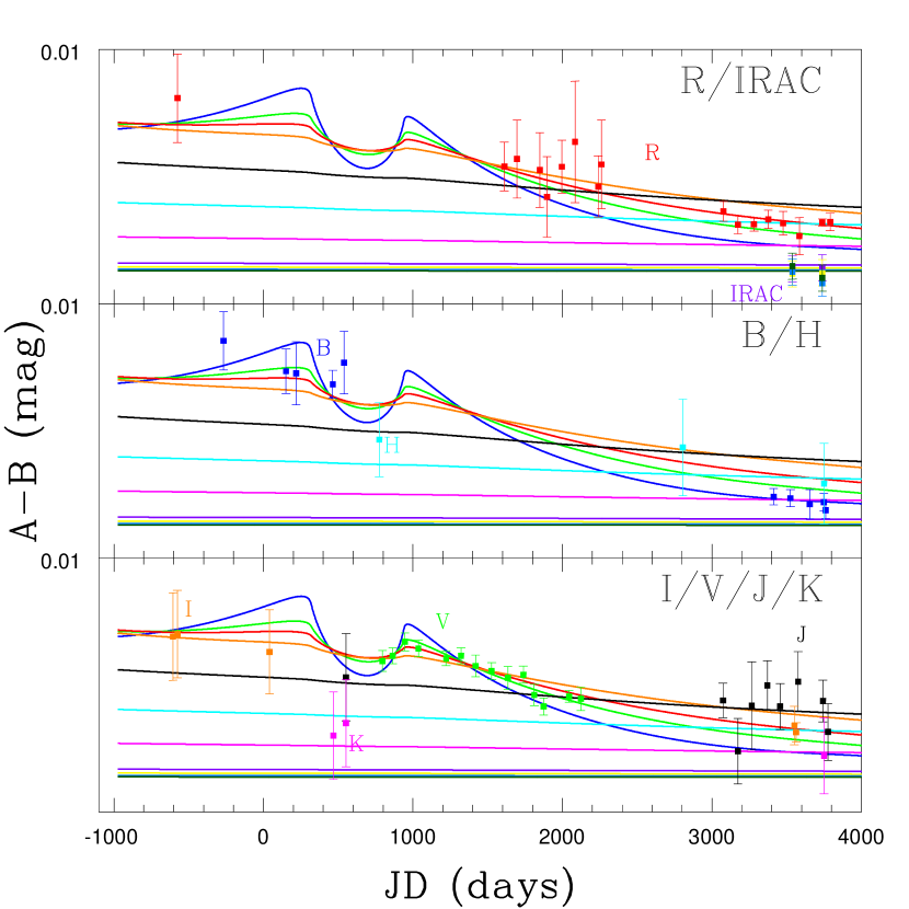
Figure 1.— The HE 1104–1805 multi-band light curves. The curves show a model for the BVRIJHK bands and the four IRAC channels ($3.6$ to $8.0~{}\mu$m). For clarity we split the data into three panels and show the B, V, R, and J-band data points in 200 day averages.

We use the lens model sequence from Poindexter et al. (2007), which consists of a de Vaucouleurs model matched to the HST observations embedded in an NFW halo, to set the shear $\gamma$, convergence $\kappa$, and stellar fraction $\kappa_{*}/\kappa$ for the microlensing magnification patterns. The models were constrained to match the flux ratios of the mid-IR IRAC bands. We used a mass function of $dN/dM\propto M^{-1.3}$ with $M_{max}/M_{min}=50$ whose structure is broadly consistent with the Galactic disk mass function of Gould (2000). The lens models were parameterized by $f_{M/L}$, the fraction of a constant mass-to-light ratio ($M/L$) represented by the visible galaxy. For each of ten models, $f_{M/L}=0.1,0.2,\ldots,1.0$, we produce 2 magnification patterns with an outer dimension of $10R_{\rm E}$ and $8192^{2}$ pixels to achieve a pixel scale of $4.4\times 10^{13}~{}(\left<M\right>/hM_{\sun})^{1/2}$ cm/pixel that is smaller than the gravitational radius $r_{g}=GM/c^{2}=3.5\times 10^{14}~{}\rm cm$ expected for HE 1104–1805 (see §3). We experimented extensively with magnification patterns of different sizes and scales to ensure that our choice of pixel scale and outer dimension did not affect our results. We used the velocity model from Kochanek (2004), where the adopted values are $73~{}\rm km/s$ for our velocity projected onto the lens plane, $308~{}\rm km/s$ for the velocity dispersion of the lens estimated from fitting an isothermal lens model and RMS peculiar velocities of $135$ and $71~{}\rm km/s$ for the lens and source respectively. We assume a uniform prior on the mean masses of the stars of $0.1~{}M_{\sun}<\left<M\right><1.0~{}M_{\sun}$, but this has only limited effects on the estimates of the disk size (see Kochanek 2004). Our estimates of the disk properties average over all these parameters.

Figure 2.— Probability distributions for the B-band accretion disk half-light radius. The bold solid (dashed) curve is the distribution based on a logarithmic (linear) prior on the disk size. The filled (open) square near the top is the median of the distribution with a logarithmic (linear) prior along with the $68\%$ confidence error bars. The lower curves show the contribution from the more significant $\beta$ trials, labeled by their value of $\beta$. The vertical lines show the B-band thin disk size predicted from the I-band flux (Eqn. 3) and the size expected from standard thin disk theory (Eqn. 2) for Eddington limited ($L/L_{\rm E}=1$) accretion with $\eta=10\%$ efficiency.

We modeled the disk as a face-on thermally radiating disk with temperature $T\propto R^{-\beta}$ (e.g. Collier et al., 1998), corresponding to a surface brightness profile of

$$f_{\nu}\propto\nu^{3}\left[\exp{(R/R_{\lambda})}^{\beta}-1\right]^{-1}$$ (1)

where the size scale is $R_{\lambda}=R_{\rm B}(\lambda/\lambda_{\rm B})^{1/\beta}$ and $R_{\rm B}$ is the disk size at the observed B-band ($1310$Å in the rest frame) and $\beta=3/4$ for standard thin disk theory. In many cases we report the half-light radius $R_{1/2,\lambda}(\beta)=C(\beta)R_{\lambda}(\beta)$ where for $\beta=3/4$, $C=2.44$. While we do not include an inner disk edge of $R_{in}\simeq 2r_{g}$ to $6r_{g}$, the lack of this central hole has little effect on our results unless $\beta\rightarrow 2$ or $R_{B}\simeq R_{in}$. We tried disk models with profile exponents of $\beta=1/4,3/8,\cdots,7/4$, making $4\times 10^{6}$ trial light curves for each value of $\beta$. In our final analysis we use the $3.3\times 10^{6}$ light curves that passed a threshold of $\chi^{2}/N_{dof}\leq 3$ for $N_{dof}=438$ degrees of freedom. We used both a logarithmic prior, $P(R_{\lambda})\propto 1/R_{\lambda}$, and a linear prior, $P(R_{\lambda})\propto\rm constant$, on the disk size. Generally, a logarithmic prior is preferred for scale free variables like $R_{\lambda}$, but for this problem a linear prior may be more appropriate for small source sizes because we are sensitive to the difference between small sizes only during caustic crossings. If, however, we have solutions with the caustic crossing sitting in a gap of the light curve, we will find that $P(D|R_{\lambda})$ approaches a constant value as $R_{\lambda}$ goes to zero. This leads to a formal divergence in $P(R_{\lambda}|D)$ with a logarithmic prior, suggesting that a linear prior may be more appropriate. In practice, Figs. 2-3 show the results for both options and we use the results for the logarithmic prior in our discussion. For the results we give the value at the median of the probability distribution and the 68% ($1~{}\sigma$) confidence regions.

3. Results and Discussion

We have no difficulty reproducing the observed light curves, including the presently observed color reversal. We illustrate this in Fig. 1, where we superpose our best fitting light curve model on the data.

Figure 3.— B-band half-light disk radius $R_{1/2,\rm B}$ versus $\beta$ where $T\propto R^{-\beta}$. The solid (dotted) contours represent the $68\%$, $90\%$, and $95\%$ confidence levels of the microlensing measurements assuming a logarithmic (linear) prior on disk size. The small solid contours is the B-band flux estimate considering a $T\propto R^{-\beta}$ model fit to all the bands. The dashed line shows the size estimated from just the B-band flux measurement without the constraint on $\beta$ from the other bands. The large solid square at $\beta=3/4$ shows the radius predicted by thin disk theory (Eqn. 2).

We find a wavelength-size scaling of the accretion disk of $\beta=0.61^{+0.21}_{-0.17}$ and $\beta=0.89^{+0.23}_{-0.16}$ for the logarithmic and linear priors respectively (Fig. 4), where $R_{\lambda}\propto\lambda^{1/\beta}$ and $T\propto R^{-\beta}$. This is consistent with simple thin disk theory ($\beta=3/4$). The B-band half light radius is $R_{1/2,\rm B}=6.7^{+6.2}_{-3.2}\times 10^{15}$ cm with the logarithmic prior and $R_{1/2,\rm B}=1.3^{+0.9}_{-0.6}\times 10^{16}$ cm with the linear prior (Figs. 2 and 3). We use the half light radius rather than $R_{\lambda}$ because it has less covariance with the exponent $\beta$. We can also estimate the sizes for the individual bands, as shown in Fig. 4, although these will be highly correlated because the model only has the exponent $\beta$ and one scale length as actual parameters. If we fix $\beta=3/4$, then we find that B-band size for this case is $R_{1/2,\rm B}(\beta=3/4)=9.0^{+6.5}_{-4.2}\times 10^{15}$ cm.

We can compare to thin disk theory only for the case of $\beta=3/4$ since there is no simple generalization for alternate values of $\beta$. Based on the CIV emission line width of HE 1104–1805, Peng et al. (2006) estimated a black hole (BH) mass of $M_{1104}=2.4\times 10^{9}M_{\sun}$, which corresponds to a gravitational radius of $r_{g}=GM/c^{2}=3.5\times 10^{14}~{}\rm cm$. In thin disk theory (Shakura & Sunyaev, 1973), this implies a size scaling of

$$\begin{split}R_{\lambda}&=\frac{1}{\pi^{2}}\left[\frac{45}{16}\frac{\lambda_{rest}^{4}r_{g}\dot{M}}{h_{p}}\right]^{1/3}\\ &=(1.7\times 10^{16})\left[\frac{\lambda_{rest}}{\mu\rm m}\right]^{4/3}\left[\frac{M_{BH}}{M_{1104}}\right]^{2/3}\left[\frac{L}{\eta L_{\rm E}}\right]^{1/3}~{}{\rm cm},\end{split}$$ (2)

where $\eta$ is the radiative efficiency ($L=\eta\dot{M}c^{2}$), $h_{p}$ is the Planck constant, and $L/L_{\rm E}$ is the fraction of the Eddington luminosity radiated by the QSO. Thus the expected B-band (rest frame $0.13~{}\mu$m) size for a disk radiating at the Eddington limit ($L/L_{\rm E}$) with 10% efficiency is $R_{\rm B}=2.4\times 10^{15}$ cm corresponding to a half-light radius of $R_{1/2,\rm B}=5.9\times 10^{15}$ cm. This agrees well with our measurement (Figs. 2, 3, and 4). For the $\beta=3/4$ model the disk scale length is significantly larger than the gravitational radius ($R_{1/2,\rm B}\sim 20r_{g}$) and corrections for the inner edge of the disk will be modest. Particularly if we allow for uncertainties in the black hole mass estimate ($\sim 0.3$ dex), there is good agreement with the simplest possible thin disk model.

Figure 4.— Half-light disk radius $R_{1/2,\lambda}$ versus wavelength. The filled squares (open triangles) are the size estimates from microlensing (the source flux, Eqn. 3). Note that the microlensing uncertainties are highly correlated because the only 2 actual variables are $R_{\rm B}$ and $\beta$. The short dashed and dotted lines are the best fit power laws to these measurements. The long dashed line shoes how the normalization of the points would shift if we use $\beta=3/4$ rather than the best fit slope of $\beta=0.55$.

The magnification-corrected flux of the quasar provides a second comparison scale under the assumption that the disk is thermally radiating. If the quasar has a magnification corrected magnitude of $m$, then

$$\begin{split}R_{\lambda}(\beta)\simeq\frac{2.8\times 10^{15}}{h\sqrt{K(\beta)\cos i}}\frac{D_{OS}}{r_{H}}\left[\frac{\lambda_{obs}}{\mu\rm m}\right]^{3/2}\\ \left[{\frac{\hbox{zpt}}{2409~{}\hbox{Jy}}}\right]^{1/2}10^{-0.2({\rm m}-19)}\hbox{cm}.\end{split}$$ (3)

where $\lambda_{obs}$ is the observed wavelength, zpt is the filter zero point (normalized to the I-band), and

$$K(\beta)=\frac{1}{2.58}\int_{0}^{\infty}udu\left[\exp(u^{\beta})-1\right]^{-1}$$ (4)

is the $\beta$-dependent term due to the temperature profile normalized so that $K(\beta=3/4)=1$. Assuming the magnifications of images A and B are 11.5 and 4 respectively (as found in the best fit macro model in Poindexter et al. 2007), we calculated the magnification corrected source magnitude in each of the 11 bands to estimate the disk size versus wavelength (Fig. 4). For the H-, I-, and V-band, we used the HST observations of Lehár et al. (2000). The mid-IR magnitudes are from Spitzer (Poindexter et al., 2007). We calibrated the SMARTS B/R and J/K data using the Guide Star Catalog and 2MASS respectively.

The sizes estimated from the flux are very well fit by a power law (see Fig. 4) with a slope equivalent to $\beta=0.55^{+0.03}_{-0.02}$ when we assume a magnification uncertainty of a factor of 2. While this slope is consistent with our microlensing results, the size scale of $R_{1/2,\rm B}=1.8^{+0.7}_{-0.5}\times 10^{15}$ is smaller by a factor of 4 than our standard estimate. This discrepancy depends on the value of $\beta$, with a flatter temperature profile showing less of a difference. While there is little extinction in the lens, 2.9 mags of B-band ($0.31~{}\mu$m rest frame) extinction in the source would reconcile the flux and microlensing size estimates. However, with such an extinction, neither SMC (Gordon et al., 2003) or AGN (Gaskell et al., 2004) extinction curves can reconcile the two estimates at all wavelengths. Nonetheless absorption in the source could be a partial explanation.

The general relationship we find between the microlensing, thin disk and flux sizes seems to be typical. Pooley et al. (2007) noted qualitatively that microlensing sizes tended to be larger than expected from the optical flux and thin disk models. Morgan et al. (2007) showed quantitatively that the microlensing sizes scaled as expected with BH mass ($R_{\lambda}\propto M^{2/3}$) and were consistent with being proportional to the flux sizes, but that the absolute scales of the microlensing sizes were slightly larger than the thin disk sizes and considerably larger than the flux sizes. Our results here suggest that part of the solution may be that the effective temperature profile is somewhat shallower than $T\propto R^{-3/4}$.

Several local estimates (Collier et al., 1999; Sergeev et al., 2005) have found UV-optical wavelength dependent time delays of nearby AGN consistent with $T\propto R^{-3/4}$. They also found the flux discrepancy, but phrased the problem as needing to put the systems at higher than expected distances (through a low value of $H_{0}$) in order to reconcile the model disk surface brightness with the observed flux.

Our current disk model is a face-on, thermally radiating disk without the central temperature depression created by the inner edge of the accretion disk (Eqn 1). Omitting the inner edge has little effect because at fixed wavelength little flux is radiated there and the finite resolution of the magnification patterns eliminates the formal surface brightness divergence in Eqn. (1). It is expected from theoretical work that microlensing is primarily sensitive to an effective smoothing area, and the resulting size estimate is only weekly sensitive to the true surface brightness profile (e.g. Mortonson, Schechter & Wambsganss, 2005; Congdon et al., 2007). Nonetheless, a clear next step is to begin interpreting the microlensing results using more realistic thin disk models (e.g. Hubeny et al., 2001) to see if adding such details alters the basic picture. The present results suggest that part of the solution may be to alter the temperature profile of the disk, perhaps through irradiation of the outer regions by the inner regions.

References

- Agol & Krolik (1999) Agol, E. & Krolik, J., 1999, ApJ, 524, 49
- Albrow et al. (2001) Albrow, M., et al. 2001, ApJ, 550, L173
- Blaes (2004) Blaes, O.M., 2004, in Les Houches Summer School LXXVIII (Springer: Berlin) 137
- Cackett et al. (2007) Cackett, E. M., Horne, K., Winkler, H., 2007, [astro-ph/0706.1464]
- Collier et al. (1998) Collier, S. J., et al. 1998, ApJ, 500, 162
- Collier et al. (1999) Collier, S., Horne, K., Wanders, I., & Peterson, B. M. 1999, MNRAS, 302, L24
- Congdon et al. (2007) Congdon, A. B., Keeton, C. R., & Osmer, S. J. 2007, MNRAS, 376, 263
- Courbin et al. (1998) Courbin, F., Lidman, C. & Magain, P., 1998, A&A, 330, 57
- Falco et al. (1999) Falco, E.E., Impey, C.D., Kochanek, C.S., Lehár, J., McLeod, B. A., Rix, H.-W., Keeton, C. R., Mu oz, J. A., Peng, C. Y., 1999, ApJ, 523, 617
- Gaskell et al. (2004) Gaskell, C. M., Goosmann, R. W., Antonucci, R. R. J., & Whysong, D. H. 2004, ApJ, 616, 147
- Gil-Merino et al. (2002) Gil-Merino, R., Wisotzki, L. & Wambsganss, J., 2002, A&A, 381, 428
- Goicoechea et al. (2004) Goicoechea, L. J., Shalyapin, V., Gonz lez-Cadelo, J., Oscoz, A., 2004, A&A, 425, 475
- Gordon et al. (2003) Gordon, K. D., Clayton, G. C., Misselt, K. A., Landolt, A. U., & Wolff, M. J. 2003, ApJ, 594, 279
- Gould (2000) Gould, A. 2000, ApJ, 535, 928
- Grieger et al. (1991) Grieger, B., Kayser, R., & Schramm, T., 1991, A&A, 252, 508
- Hubeny et al. (2001) Hubeny, I., Blaes, O., Krolik, J. H., & Agol, E. 2001, ApJ, 559, 680
- Kochanek (2004) Kochanek, C.S., 2004, ApJ, 605, 58
- Kochanek & Dalal (2004) Kochanek, C.S., Dalal, N., 2004, ApJ, 610, 69
- Kochanek et al. (2007) Kochanek, C.S., Dai, X., Morgan, C., Morgan, N., Poindexter, S. & Chartas, G., 2007, in Statistical Challenges in Modern Astronomy IV in Statistical Challenges in Modern Astronomy IV G. J. Babu and E. D. Feigelson, eds., (Astron. Soc. Pacific: San Francisco), [astro-ph/0609112]
- Lehár et al. (2000) Lehár, J., et al., 2000, ApJ, 536, 584
- Morgan et al. (2007) Morgan, C., Kochanek, C.S., Morgan, N.D., Falco, E.E., 2007, in preparation
- Mortonson, Schechter & Wambsganss (2005) Mortonson, M.J., Schechter, P.L., Wambsganss, J., 2005, ApJ, 628, 594
- Ofek & Maoz (2003) Ofek, E.O. & Maoz, D., 2003, ApJ, 594, 101
- Peng et al. (2006) Peng, C.Y., Impey, C.D., Rix, H.-W., Kochanek, C.S., Keeton, C.R., Falco, E.E., Lehár, J. & McLeod, B.A., 2006, ApJ, 649, 616
- Poindexter et al. (2007) Poindexter, S., Morgan, N., Kochanek, C. S., & Falco, E. E. 2007, ApJ, 660, 146
- Pooley et al. (2007) Pooley, D., Blackburne, J. A., Rappaport, S., & Schechter, P. L. 2007, ApJ, 661, 19
- Sergeev et al. (2005) Sergeev, S. G., Doroshenko, V. T., Golubinskiy, Y. V., Merkulova, N. I., & Sergeeva, E. A. 2005, ApJ, 622, 129
- Shakura & Sunyaev (1973) Shakura, N.I. & Sunyaev, R.A., 1973, A&A, 24, 337
- Schechter et al. (2003) Schechter, P.L., et al. 2003, ApJ, 584, 657
- Remy et al. (1998) Remy, M., Claeskens, J.-F., Surdej, J., Hjorth, J., Refsdal, S., Wucknitz, O., Sørensen, A.N. & Grundahl, F., 1998, New Astronomy, 3, 379
- Wambsganss (2006) Wambsganss, J, 2006, in Gravitational Lensing: Strong Weak and Micro, Saas-Fee Advanced Course 33, G. Meylan, P. North, P. Jetzer, eds., (Springer: Berlin) 453, [astro-ph/0604278]
- Wisotzki et al. (1993) Wisotzki, L., Köhler, R., Kayser, R. & Reimers, D., 1993, A&A, 278, L15
- Wyrzykowski et al. (2003) Wyrzykowski, Ł. et al., 2003, Acta Astronomica, 53, 229