Manifestation of nonequilibrium initial conditions in molecular rotation: the generalized J-diffusion model

Abstract

In order to adequately describe molecular rotation far from equilibrium, we have generalized the J-diffusion model by allowing the rotational relaxation rate to be angular momentum dependent. The calculated nonequilibrium rotational correlation functions (CFs) are shown to decay much slower than their equilibrium counterparts, and orientational CFs of hot molecules exhibit coherent behavior, which persists for several rotational periods. As distinct from the results of standard theories, rotational and orientational CFs are found to dependent strongly on the nonequilibrium preparation of the molecular ensemble. We predict the Arrhenius energy dependence of rotational relaxation times and violation of the Hubbard relations for orientational relaxation times. The standard and generalized J-diffusion models are shown to be almost indistinguishable under equilibrium conditions. Far from equilibrium, their predictions may differ dramatically.

I Introduction

There have been collected many evidences (due to polarization time-resolved experiments, ruh93 ; wie93 ; wie96 ; zew96 ; hoc96 ; hoc97 ; hoc97a ; voh98 ; voh99 ; voh99a ; vol99 ; voh00 ; voh00a ; nib01 ; bra03 computer simulations, wil89 ; ger94 ; ben93 ; ben95 ; ben03 ; gri84 and model studies gri84 ; gel00 ; gel01 ) which indicate that rotational and orientational relaxations of molecules in liquids under equilibrium and (highly) nonequilibrium conditions differ significantly. The studies of nonequilibrium rotational relaxation have recently culminated in papers. str06 ; str06a As has been demonstrated, relaxation of rotational energy of hot nonequilibrium photofragments slows significantly with the increase of their initial rotational temperature and differs dramatically from relaxation of the equilibrium rotational energy correlation function, manifesting thereby breakdown of the linear response description. Furthermore, hot nonequilibrium molecules exhibit almost dissipation-free coherent rotation, which persists for several rotational periods. Molecular dynamic simulations have attributed this unusual behavior to a rapid rearrangement of the local liquid structure: a hot solute pushes away the neighboring solvent molecules and rotates almost freely until it looses enough energy. str06 ; str06a Another way of thinking about that is in terms of the angular momentum dependent rotational friction: highly rotationally excited molecules experience lower friction than their thermally equilibrated counterparts. str06a ; kos06d

These nonequilibrium relaxations are not reproduced by conventional theories of (equilibrium) molecular rotation, which are based upon master equations with constant relaxation rates (the extended diffusion models, gor66 ; rid69 ; McCl77 ; BurTe the Keilson-Storer model sack ; BurTe ; kos06 ) or rotational Fokker-Planck equations with constant frictions. hub72 ; McCo ; mor82 ; McCl87 Physically, this is not surprising. If we consider relaxation under equilibrium conditions, then all the relevant energies are of the order of $k_{B}T$ ($k_{B}$ being the Boltzmann constant and $T$ being the temperature of the bath). So, putting aside non-Markovian effects, we can always introduce a certain effective constant relaxation rate. If we consider relaxation under nonequilibrium conditions, when initial energies are much higher than $k_{B}T$, such a description is no longer applicable, and the angular momentum dependence of relaxation rates must be explicitly taken into consideration (see Ref. str06a ; kos06d for more detailed argumentation and discussion).

There exist two major and complimentary approaches to rotational relaxation, via the Fokker-Planck equations hub72 ; McCo ; mor82 ; McCl87 and extended diffusion models. gor66 ; rid69 ; McCl77 ; BurTe In our previous paper, kos06d we have demonstrated how the angular-momentum dependent friction can be incorporated into the rotational Fokker-Planck equation. The present paper deals with a similar generalization of the J-diffusion model. First, we investigate how the angular momentum dependent rates manifest themselves in relaxations of initial nonequilibrium distributions and in behaviors of rotational and orientational correlation functions (CFs). Second, we develop a reliable tool for the description of nonequilibrium molecular rotation, which can be used i.e. for the interpretation of photofragment anisotropy decays. ruh93 ; wie93 ; wie96 ; zew96 ; hoc96 ; hoc97 ; hoc97a ; voh98 ; voh99 ; voh99a ; vol99 ; voh00 ; voh00a ; nib01 ; bra03 Third, we demonstrate how the use of standard ”equilibrium” approaches may lead to quantitatively and even qualitatively wrong results, if they are applied to describe nonequilibrium molecular rotation.

Photodissociation $\mathrm{ICN}+h\nu\rightarrow\mathrm{CN+I}$ (which was studied experimentally in the gas-phase zew94 ; zew01 ; wit85 and in the condensed phase zew96 ; bra03 , and also investigated via computer simulations wil89 ; ger94 ; ben95 ; ben03 ; str06 ; str06a ) is chosen in the present article as a prototype process which produces highly nonequilibrium hot photofragments. The results of the molecular dynamics simulations str06 ; str06a are used to obtain realistic values of the model parameters and to test our theoretical predictions.

The structure of our paper is as follows. The generalized J-diffusion model, which accounts for the angular momentum dependence of the relaxation rate, is developed in Sec. 2. A convenient explicit expression for the initial nonequilibrium angular momentum distribution is derived in Section 3. Relaxation of this nonequilibrium distribution, as well as dynamics of the angular momentum and energy CFs, are investigated in Section 4. Orientational relaxation is studied in Section 5. The Appendixes describe the methods of calculation of rotational CFs (A), their relaxation times (B), and orientational CFs (C).

The reduced variables are used throughout the article: time, angular momentum and energy are measured in units of $\sqrt{I/(k_{B}T})$, $\sqrt{Ik_{B}T}$ and $k_{B}T$, respectively. Here $k_{B}$ is the Boltzmann constant, $T$ is the temperature of the equilibrium bath, and $I$ is the moment of inertia of the photofragment, so that $\tau_{r}=\sqrt{I/(k_{B}T})$ is the averaged period of its free rotation. For CN at $300$ K, $\tau_{r}=$$0.2$ ps. All the Laplace-transformed operators are denoted by tilde, viz.

$$\tilde{f}(s)\equiv\int_{0}^{\infty}dt\exp\{-st\}f(t)\,\,\mathrm{for}\,\,\forall\,f(t).$$ (1)

II Generalized J-diffusion model

Restricting our consideration to linear molecules and neglecting the short-time non-Markovian effects, we start from the rotational master equation

$$\partial_{t}\rho(\mathbf{J},\mathbf{\Omega},t)=-i\mathbf{J}\hat{\mathbf{L}}\rho(\mathbf{J},\mathbf{\Omega},t)-\int d\mathbf{J}^{\prime}T(\mathbf{J}^{\prime}|\mathbf{J})\rho(\mathbf{J},\mathbf{\Omega},t)+\int d\mathbf{J}^{\prime}T(\mathbf{J}|\mathbf{J}^{\prime})\rho(\mathbf{J}^{\prime},\mathbf{\Omega},t).$$ (2)

Here $\rho(\mathbf{J},\mathbf{\Omega},t)$ is the probability density function, $\mathbf{J}$ is the (two-dimensional) angular momentum of the linear top in its molecular frame, $\mathbf{\Omega}$ are the Euler angles which specify orientation of the molecular frame with respect to the laboratory one. The first term on the right-hand side of Eq. (2) is the free-rotor Liouville operator, which describes the angular momentum driven reorientation, $\hat{\mathbf{L}}$ being the angular momentum operator in the molecular frame. The last two terms are responsible for the bath-induced relaxation. Since our molecular ensemble is isotropic, the kernel of the dissipation operator, $T(\mathbf{J}|\mathbf{J}^{\prime})$, is $\mathbf{\Omega}$-independent. It must obey the detailed balance

$$T(\mathbf{J}|\mathbf{J}^{\prime})\rho_{B}(\mathbf{J}^{\prime})=T(\mathbf{J}^{\prime}|\mathbf{J})\rho_{B}(\mathbf{J}),$$ (3)

which is responsible for bringing the system under study to the equilibrium rotational Boltzmann distribution

$$\rho_{B}(\mathbf{J})=(2\pi)^{-1}\exp\{-\mathbf{J}^{2}/2\}.$$ (4)

Normalization of Eq. (2),

$$\int d\mathbf{J}d\mathbf{\Omega}\rho(\mathbf{J},\mathbf{\Omega},t)\equiv 1,$$ (5)

which insures conservation of probability, is accounted for automatically.

By selecting a particular form of the relaxation kernel $T(\mathbf{J}^{\prime}|\mathbf{J})$, one can recover many models of rotational relaxation available in the literature: the extended diffusion models, gor66 ; rid69 ; McCl77 ; BurTe the rotational Fokker-Planck equation, hub72 ; McCo ; mor82 ; McCl87 the Keilson-Storer model. sack ; BurTe ; kos06 All these models, however, yield $\int d\mathbf{J}^{\prime}T(\mathbf{J}^{\prime}|\mathbf{J})=\nu=\textrm{const}$, that is the collision rate is angular momentum independent. For example, the most popular model of rotational relaxation, the J-diffusion model, corresponds to the choice

$$T(\mathbf{J}|\mathbf{J}^{\prime})=\nu\rho_{B}(\mathbf{J}).$$ (6)

We cannot straightforwardly generalize the J-diffusion model by replacing the rate $\nu$ with its $J$-dependent counterpart $\nu(J)$, since this procedure would violate normalization (and therefore conservation) of the probability density (Eq. (5)). To get a correct description, we assume that the relaxation kernel can be represented in the factorized Gaussian form

$$T(\mathbf{J}|\mathbf{J}^{\prime})=\exp\{-a\mathbf{J}^{2}/2\}\exp\{-b\mathbf{J^{\prime}}^{2}/2\}c,$$ (7)

$a,\,b$, and $c$ being numerical constants to be specified. To satisfy the detailed balance (3), we must choose

$$a=1+b.$$ (8)

Then the generalized J-diffusion relaxation kernel takes the form

$$T(\mathbf{J}|\mathbf{J}^{\prime})=\nu\frac{1+b}{2\pi}\exp\{-(1+b)\mathbf{J}^{2}/2\}\exp\{-b\mathbf{J^{\prime}}^{2}/2\}.$$ (9)

Here the rate $\nu$ governs the dissipation strength and the constant

$$c=\nu\frac{1+b}{2\pi}$$ (10)

is chosen to insure that

$$\int d\mathbf{J}^{\prime}T(\mathbf{J}^{\prime}|\mathbf{J})\equiv\nu z(J),\,\,\,z(J)\equiv\exp\{-bJ^{2}/2\}.$$ (11)

Thus, $\nu z(J)$ can be regarded as $J$-dependent collision frequency. FootG

Eq. (7) looks as a natural generalization of the standard J-diffusion kernel (6), which still preserves its Gaussian and factorized form. If $b$ is small (it is indeed small, see bellow), then the kernel (7) can be regarded as the first order correction to its J-diffusion counterpart (6). Furthermore, any relaxation kernel $T(\mathbf{J}^{\prime}|\mathbf{J})$ can be expanded in series on Gaussians,

$$T(\mathbf{J}|\mathbf{J}^{\prime})=\sum_{b}\nu_{b}\frac{1+b}{2\pi}\exp\{-(1+b)\mathbf{J}^{2}/2\}\exp\{-b\mathbf{J^{\prime}}^{2}/2\},$$ (12)

$\nu_{b}$ being certain expansion coefficients. foot3 Thus, Eq. (7) retains the first term in this expansion, and can further be refined by taking more terms, if necessary. The use of Eq. (7) can be justified a posteriori, since the predictions of the generalized J-diffusion model in Secs. 4 and 5 sustain comparison with the results of molecular dynamics simulations performed in Refs. str06 ; str06a

Plugging the kernel (7) into Eq. (2) we obtain our generalized J-diffusion master equation:

$$\partial_{t}\rho(\mathbf{J},\mathbf{\Omega},t)=-i\mathbf{J}\hat{\mathbf{L}}\rho(\mathbf{J},\mathbf{\Omega},t)-\nu z(J)\rho(\mathbf{J},\mathbf{\Omega},t)$$

$$+\nu(1+b)z(J)\rho_{B}(\mathbf{J})\int d\mathbf{J}^{\prime}z(J^{\prime})\rho(\mathbf{J}^{\prime},\mathbf{\Omega},t).$$ (13)

This is the equation which will be studied in the subsequent Sections. When $b=0$ ($z=1$), it reduces to the standard J-diffusion model.

Before embarking at particular calculations, it is useful to estimate plausible values of the parameters $\nu$ and $b$. Since $\nu$ describes the overall dissipation strength and is similar to its counterpart in the standard J-diffusion model, there are no intrinsic limitations on the value of this parameter. It is small ($<1$) for rarefied gases and large ($>1$) for liquids and solutions. As to the value of $b$, it is expected to be small ($\ll 1$), since the effects due to the $J$-dependence of relaxation rates do not manifest themselves at room temperatures under equilibrium conditions. On the other hand, if the initial nonequilibrium energy of the photofragment $E_{\Delta}$ is much larger than $k_{B}T$, then the product $b(E_{\Delta}/k_{B}T)$ is not necessarily small. It is in this case the effects due to the $J$-dependence of relaxation rates become important. Note that the parameters $\nu$ and $b$ must be independent of initial conditions. However, as we shall see in Secs. 4 and 5, Eq. (13) predicts that nonequilibrium responses, i.e. the ensuing rotational and orientational CFs, depend strongly upon initial conditions.

III Nonequilibrium initial distribution

Normally, master equations like (13) are used to calculate various rotational and orientational CFs under equilibrium conditions, assuming that $\rho(\mathbf{J},\mathbf{\Omega},0)=(2\pi)^{-3}\rho_{B}(\mathbf{J})$. We wish to study rotational relaxation under nonequilibrium initial conditions

$$\rho(\mathbf{J},\mathbf{\Omega},0)=(2\pi)^{-3}\rho_{ne}(\mathbf{J}).$$ (14)

To get an explicit expression for $\rho_{ne}(\mathbf{J})$, we adopt a model developed in Ref. gel02 Let us consider the photoreaction $A+h\nu\rightarrow B+\mathrm{products}$. We assume that the photofragmentation is instantaneous on the time scale of molecular rotation. This assumption holds true for most of small wil89 ; ger94 ; ben93 ; ben95 ; ben03 ; zew94 ; zew01 and polyatomic gel99 molecules, for which the photofragmentation time can be be estimated by few hundreds of femtoseconds. FootA Having accepted the assumption about an instantaneous (impulsive) photodecomposition, we immediately conclude that dissociation produces a nonequilibrium distribution over the angular momenta of photoproducts. Indeed, there exist two major sources of rotational excitation of fragments. These are the parent molecule rotation and the applied torque. Therefore, the angular momenta of the parent ($\mathbf{J}_{A}$) and product ($\mathbf{J}_{B}$) molecules are connected through the formula zew94 ; gel99

$$J_{B,\alpha}=\sum_{\alpha=x,y,z}I_{B,\alpha}R_{\alpha\beta}(\mathbf{\Xi})I_{A,\beta}^{-1}J_{A,\beta}+\Delta_{\alpha}.$$ (15)

The first term describes mapping of the parent molecule rotation into that of the product, and the angular momentum $\mathbf{\Delta}$ originates from the impulsive torque arising due to the rupture of chemical bond(s) of the parent. The small Latin indexes label the Cartesian components of the corresponding vectors and tensors, $I_{A,\alpha}$ and $I_{B,\alpha}$ are the main moments of inertia of the species A and B, $R_{\alpha\beta}(\mathbf{\Xi})$ is the matrix of rotation from the frame of the main moments of inertia of the product to that of the parent, and $\mathbf{\Xi}$ are the pertinent Euler angles.

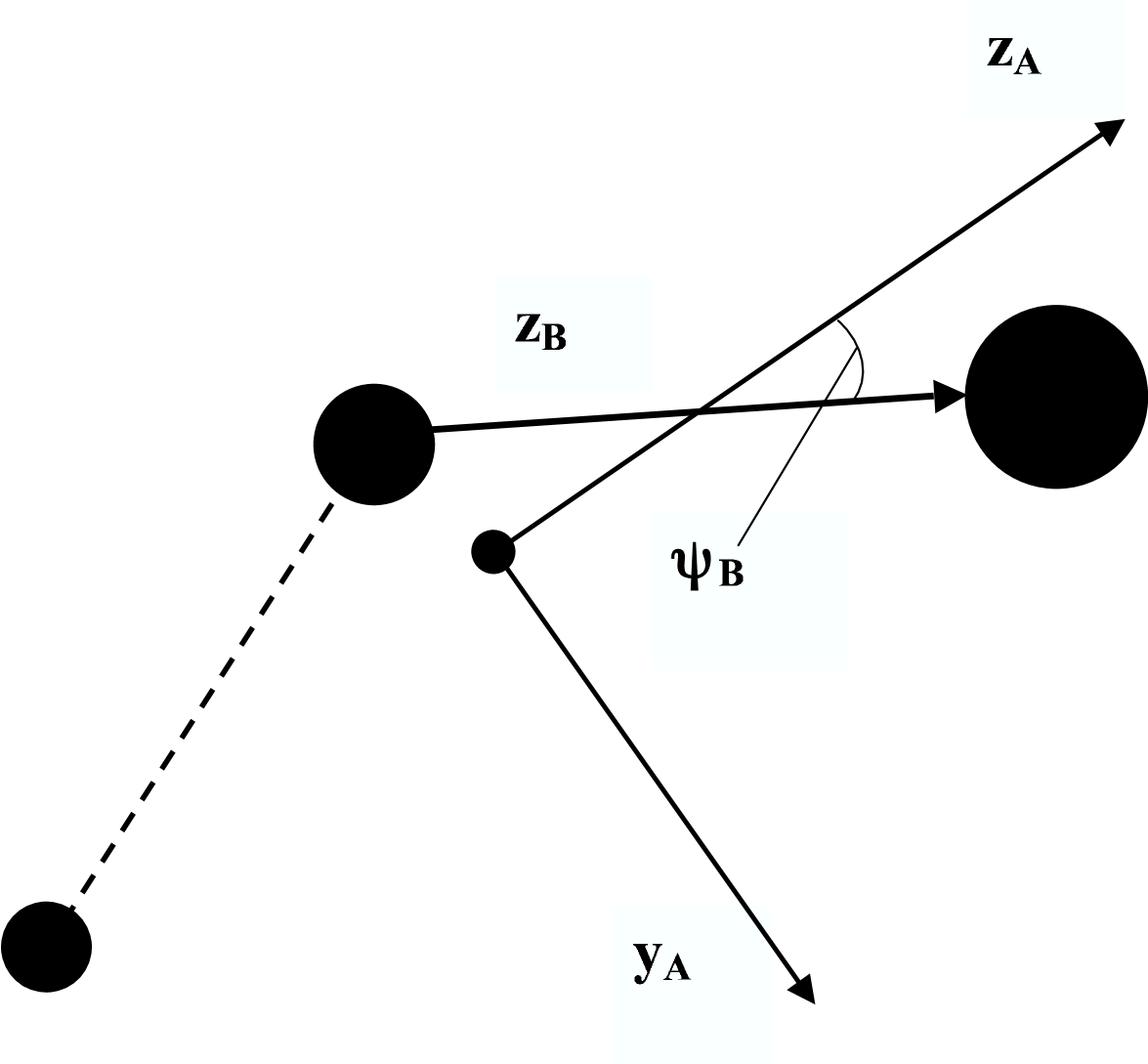
Figure 1: Sketch of the dissociating triatomic molecule.

Let the parent molecule A be a planar asymmetric top (i.e., a triatomic molecule, $I_{A,x}=I_{A,y}+I_{A,z}$) and the product B be a linear rotor ($I_{B,x}=I_{B,y}=I_{B},\,\,I_{B,z}=0$). We then define the molecular frames of the parent ($x_{A},\,y_{A},\,z_{A}$) and product ($x_{B},\,y_{B},\,z_{B}$) molecules in such a way that the axes $x_{A}||x_{B}$ are perpendicular to the plane of the parent molecule, and $z_{B}$-axis coincides with that of the linear fragment (see Fig. 1). In this case

$$R(\mathbf{\Xi})=\left(\begin{array}[]{ccc}1&0&0\\ 0&\cos(\psi_{B})&\sin(\psi_{B})\\ 0&-\sin(\psi_{B})&\cos(\psi_{B})\end{array}\right),$$ (16)

$\psi_{B}=\angle(y_{A}y_{B})=\angle(z_{A}z_{B})$. It is natural to surmise that the applied torque is perpendicular to the plane of the parent molecule, $\mathbf{\Delta}||x_{B}$. Then, assuming that the parent molecules have a Boltzmann equilibrium distribution at the bath temperature $T$, we find that the linear photoproducts are distributed according to gel02

$$\rho_{ne}(\mathbf{J})=\frac{\xi\eta}{2\pi^{2}}\int_{0}^{\pi}d\theta\exp\left\{-\frac{\eta}{2}\left([J\cos\theta+\Delta]^{2}+\xi^{2}J^{2}\sin^{2}\theta\right)\right\}$$ (17)

(hereafter, the subscript B, which denotes the angular momentum and moment of inertia of fragment B, is omitted and $\Delta$ is the magnitude of the impulsive angular momentum $\mathbf{\Delta}$). We have introduced the parameters foot2

$$\eta=\frac{I_{A,x}}{I},\,\,\,\xi^{2}=\frac{1}{I_{A,x}\{\cos^{2}(\psi_{B})/I_{A,y}+\sin^{2}(\psi_{B})/I_{A,z}\}}.$$ (18)

Eq. (18) is a desirable nonequilibrium distribution, which is employed in all the subsequent calculations. The entire information about dissociation is contained in the parameters $\Delta$, $\eta$, and $\xi$. The first of them is responsible for the applied torque and can be considered as dynamical. The last two parameters control the parent-product rotational energy transfer. They are determined by the geometry of the dissociating molecule. Note that $0\leq\xi\leq 1$. When $\xi\approx 0$, then the parent molecule is highly prolate ($I_{A,z}\ll I_{A,x},\,I_{A,y}$) and the linear fragment is ”attached” perpendicularly to the parent molecule axis ($\psi_{B}\approx\pi/2$). If $\xi\approx 1$, then the parent molecule is also considerably prolate, but the linear fragment is ”attached” parallel to the parent molecule axis ($\psi_{B}\approx 0$). If the parent molecule is a symmetric top ($I_{A,x}=I_{A,y}$), then $\xi=1$. The quantities $\eta$ and $\xi$ can be regarded as known for a particular photoreaction, since the angle $\psi_{B}$ and the main moments of inertia are fixed for specific molecules A and B. The value of $\Delta$ can be estimated through the consideration of the energy partitioning in the course of the photofragmentation. zew94

Distribution (18) is convenient for the further use, since it covers many different scenario of the photofragmentation. It reduces to the Boltzmann equilibrium distribution (4) if $\Delta=0$ and $\eta=$$\xi=1$. On the other hand, we get the delta-distribution

$$\rho_{ne}(\mathbf{J})=\frac{1}{2\pi}\frac{\delta(J-\Delta)}{J}$$ (19)

in the limit $\eta\rightarrow\infty$.

The quantum version of distribution (17) is immediately written down after the “quantization” of the angular momentum: gel02

$$\rho_{ne}^{Q}(j)=Z_{Q}^{-1}\chi(j),\,\,Z_{Q}=\sum_{j=0}^{\infty}\chi(j),$$ (20)

$$\chi(j)=(2j+1)\int_{0}^{\pi}d\theta\exp\left\{-\frac{\eta_{Q}}{2}\left([\overline{j}\cos\theta+\delta]^{2}+\xi^{2}\overline{j}^{2}\sin^{2}\theta\right)\right\}.$$

Here $j$ is the rotational quantum number,

$$\overline{j}=\sqrt{j(j+1)},\,\,\,\delta=\Delta/\zeta,\,\,\,\eta_{Q}=\zeta^{2}\eta,\,\,\,\zeta\equiv\hbar/\sqrt{Ik_{B}T}.$$ (21)

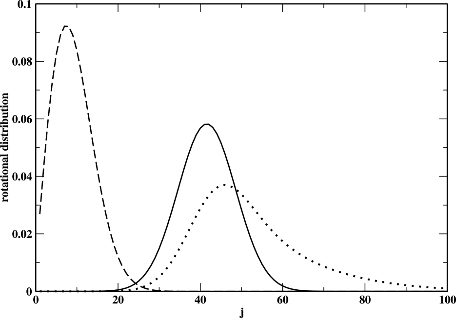
Figure 2: Rotational distributions for hot photofragments calculated for $\eta_{Q}=0.02,\,\xi=1$, $\delta=40$ (full line), $\eta_{Q}=0.02,\,\xi=0.2$, $\delta=40$ (dotted line). The equilibrium Boltzmann distribution for CN at $300$ K is depicted by dashed line ($\eta_{Q}=0.018,\,\xi=1$, $\delta=0$).

Eq. (20) allows us to simulate a rotational distribution of any width centered at any value of $j$. Several characteristic shapes of $\rho_{ne}^{Q}(j)$ are presented in Fig. 2. If $\xi=1$, the distribution is symmetric. If $\xi<1$ (for triatomics, this corresponds to dissociation from a bent configuration) the distribution becomes asymmetric, with a long-$j$ bias.

Let us now apply the above machinery to photodissociation $\mathrm{ICN}+h\nu\rightarrow\mathrm{CN+I}$. This reaction proceeds via two channels, producing low energy and high energy photofragments. The quantum distribution $\rho_{ne}^{Q}(j)$ for nascent CN-fragments has been measured in. wit85 A comparison of the “full line” distribution in Fig. 2 with that reported in wit85 reveals that the former reproduces qualitatively the experimental results for hot photofragments. For CN at $300$ K, $\zeta=0.135$. Therefore, the “realistic values” of the dimensionless parameters $\eta=\eta_{Q}/\zeta^{2}=1.1$, $\Delta=\delta\zeta=5.4$ will be used in our illustrative calculations. FootC

IV Rotational relaxation

In this section, we study evolution of the quantities which depend on the angular momentum $\mathbf{J}$ but are independent of the Euler angles $\mathbf{\Omega}$. We thus can integrate Eq. (13) over $\mathbf{\Omega}$ and arrive at the reduced master equation

$$\partial_{t}\rho(\mathbf{J},t)=-\nu z(J)\rho(\mathbf{J},t)+\nu(1+b)z(J)\rho_{B}(J)\int d\mathbf{J}^{\prime}z(J^{\prime})\rho(\mathbf{J}^{\prime},t).$$ (22)

This equation can be used, for example, to calculate the angular momentum CF

$$C_{J}(t)=\frac{\left\langle\mathbf{JJ}(t)\right\rangle_{ne}}{\left\langle\mathbf{J}^{2}\right\rangle_{ne}},$$ (23)

the averaged rotational energy

$$C_{S}(t)=\frac{\left\langle E(t)\right\rangle_{ne}-\left\langle E\right\rangle_{B}}{\left\langle E\right\rangle_{ne}-\left\langle E\right\rangle_{B}},$$ (24)

and the rotational energy CF

$$C_{E}(t)=\frac{\left\langle EE(t)\right\rangle_{ne}-\left\langle E\right\rangle_{B}\left\langle E\right\rangle_{ne}}{\left\langle E^{2}\right\rangle_{ne}-\left\langle E\right\rangle_{B}\left\langle E\right\rangle_{ne}}.$$ (25)

Here

$$E\equiv\mathbf{J}^{2}/2$$ (26)

and we use the notation $\left\langle...\right\rangle_{a}=\int d\mathbf{J}\rho_{a}(\mathbf{J})...$, $a=B,\,ne$. The corresponding integral relaxation times are determined as

$$\tau_{a}=\int_{0}^{\infty}dtC_{a}(t),\,\,\,\,\,a=J,\,E,\,S.$$ (27)

As is shown in Appendix A, the Laplace images of the probability density $\rho(\mathbf{J},t)$, as well as of CFs (23)-(25) can be given in quadratures (Eqs. (61), (45), and (53)) for any initial nonequilibrium distribution $\rho_{ne}(\mathbf{J})$. The inversion of the Laplace transforms into the time domain can elementary be performed numerically. Furthermore, we derive elucidating analytical expressions in several important particular cases, which help us to grasp essential features of rotational relaxation under nonequilibrium conditions.

Let us assume that the nonequilibrium distribution is given by Eq. (19), that is the photoproducts are produced with a fixed magnitude of the angular momentum $\Delta$. Such a situation corresponds to the procedure of the (microcanonical) preparation of hot molecules in simulations reported in str06 ; str06a . We thus define the nonequilibrium photofragment energy

$$E_{\Delta}=\Delta^{2}/2.$$ (28)

We assume, in addition, that $b$ is small ($b\ll\eta,\,\eta\xi^{2}$) but the product $bE_{\Delta}$ can take any value. Then Eq. (60) predicts that the CFs (23)-(25) are all the same and exponential,

$$C_{a}(t)=\exp\{-\nu z(\Delta)t\},\,\,\,\,\,a=J,\,E,\,S.$$ (29)

The $J$-dependent rates (11) are seen to slow rotational relaxation. The corresponding relaxation times (27) read

$$\tau_{a}=\frac{1}{\nu z(\Delta)}\equiv\frac{1}{\nu}\exp\left\{\frac{bE_{\Delta}}{k_{B}T}\right\}.$$ (30)

The last term in this expression is written in dimensional units, to emphasize that the generalized J-diffusion model predicts the Arrhenius energy dependence of the rotational relaxation times. Eq. (30) corroborates the finding str06 ; str06a ; kos06d that there exist characteristic “nonequilibrium energy” $\overline{E}_{\Delta}$ and “nonequilibrium temperature” $\overline{T}_{\Delta}=\overline{E}_{\Delta}/k_{B}$,

$$\overline{E}_{\Delta}\sim k_{B}T/b,\,\,\,\overline{T}_{\Delta}\sim T/b$$ (31)

starting from which the $J$-dependence of rotational relaxation becomes important. If the characteristic nonequilibrium energy $E_{\Delta}$ is much larger than $k_{B}T$, then the relaxation times for hot photofragments can substantially be longer than their equilibrium counterparts $\tau_{a}=1/\nu$, despite $b$ is small. The standard J-diffusion model, on the contrary, predicts that any rotational CF (41) decays exponentially with the rate $\nu$, irrespective of particular forms of $A(\mathbf{J})$, $B(\mathbf{J})$, and $\rho_{ne}(\mathbf{J})$ (see Eq. (59)). It is thus inadequate under highly nonequilibrium conditions, when $bE_{\Delta}>1$.

The Arrhenius energy dependence of the rotational relaxation times correlates with the results of Tao and Stratt, str06 ; str06a who simulated CFs $C_{S}(t)$ (24) for different initial nonequilibrium temperatures $\overline{T}_{\Delta}$. They obtained the following values: (a) $\tau_{S}=5.29$ for $\overline{T}_{\Delta}=1917$ K, (b) $\tau_{S}=7.73$ for $\overline{T}_{\Delta}=2395$ K, (c) $\tau_{S}=11.25$ for $\overline{T}_{\Delta}=2875$ K (see also Ref. kos06d ). We can take any two sets of $\tau_{S}$ and $\overline{T}_{\Delta}$ to calculate $\nu$ and $b$ by using Eq. (30). Doing so for three different pairings of the sets, we have got remarkably consistent results: $\nu=0.87$, $b=0.095$ for sets a&b, $\nu=0.84$, $b=0.094$ for sets b&c, $\nu=0.86$, $b=0.095$ for sets c&a. If we recall that Eqs. (29) and (30) are approximate and valid in the limit of $b\ll 1$, $\eta\gg 1$, the agreement becomes even more encouraging. Thus the quantity $z(\Delta)$ is close to $1$ ($0.91$) at equilibrium ($\overline{T}_{\Delta}=120$ K), $0.22$ at $\overline{T}_{\Delta}=1917$ K , $0.15$ at $\overline{T}_{\Delta}=2395$ K, and $0.11$ at $\overline{T}_{\Delta}=2875$. So, rotational relaxation at $\overline{T}_{\Delta}=2875$ K is nine times slower than that at the equilibrium temperature. Summarizing, the value of $b=0.1$ is a “realistic value” for the parameter which is responsible for the $J$-dependent relaxation.

It is timely to present an exact expression for the angular momentum integral relaxation time, which is valid for any values of the parameters of the generalized J-diffusion model. According to the formulas derived in Appendix B,

$$\tau_{J}=\frac{1}{\nu}\frac{\xi\eta}{\sqrt{(\eta-b)(\eta\xi^{2}-b)}}\frac{v(b)}{v(0)}\exp\left\{\frac{\eta bE_{\Delta}}{(\eta-b)}\right\}$$ (32)

($v(b)$ is defined via Eq. (70)). If we assume that $b\ll\eta,\,\eta\xi^{2}$, then Eq. (32) reduces to (30) for any $\eta,\,\xi$, and $\Delta$. This lends an additional support to the validity of Eqs. (30).

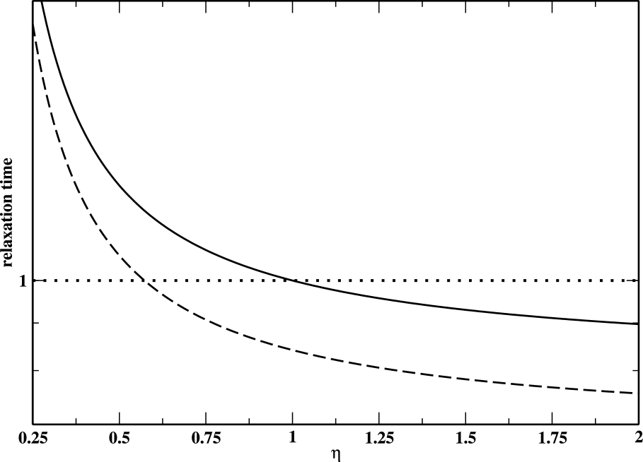
Figure 3: Reduced angular momentum relaxation time $\tau_{J}/\tau_{J}^{eq}$ (full line) and rotational energy relaxation time $\tau_{S}/\tau_{S}^{eq}$ (dashed line) vs. parameter $\eta$ calculated in the generalized J-diffusion model ($b=0.1$) for $\xi=1$ and $\Delta=0$. The dotted line corresponds to the situation when the reduced value of the relaxation times equals $1$.

On the other hand, Eq. (32) demonstrates that the $J$-dependence of rotational relaxation rates works both ways: if $\Delta$ is small and $\eta<1$, then nonequilibrium integral relaxation times can be smaller then their equilibrium counterparts. This is illustrated by Fig. 3, which shows the reduced angular momentum relaxation time $\tau_{J}/\tau_{J}^{eq}$ (full line) and rotational energy relaxation times $\tau_{S}/\tau_{S}^{eq}$ (dashed line) vs. parameter $\eta$. The nonequilibrium relaxation times are calculated via Eqs. (66)-(71), and their equilibrium counterparts are given by Eqs. (74). The observed decrease of the relaxation times at $\Delta\ll 1$ and $\eta<1$ is not so pronounced as their exponential increase at $\Delta\gg 1$.

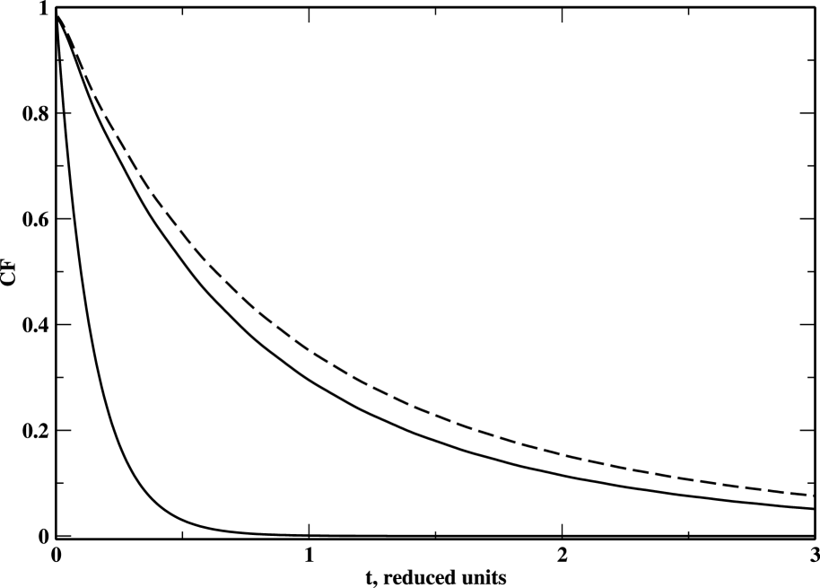
Figure 4: Angular momentum CFs $C_{J}(t)$ (full lines) and rotational energy CF $C_{E}(t)$ (dashed line) calculated for the “realistic values” of the model parameters ($\eta=1.1$, $\xi=1$, $\Delta=5.4$) and $\nu=1$. The lower line corresponds to the standard J-diffusion model ($b=0$) and the upper lines correspond to the generalized J-diffusion model ($b=0.1$).

Fig. 4 compares rotational CFs (23)-(25) calculated within the standard ($b=0$) and generalized ($b=0.1$) J-diffusion models. The CFs have been computed as explained in Appendix A. The realistic values of the model parameters ($\eta=1.1$, $\xi=1$, $\Delta=5.4$, and $\nu=1$) have been used. The standard J-diffusion predicts all the CFs to coincide with $\exp\{-\nu t\}$. According to the generalized J-diffusion model, the CFs relax much slowly, as expected. For the model parameters chosen, $C_{S}(t)$ and $C_{J}(t)$ are almost indistinguishable, FootF while $C_{E}(t)$ decays slower than the former two CFs.

If we assume that the initial distribution is given by delta-function (19) and $b\ll\eta,\,\eta\xi^{2}$, then the general Eqs. (61) and (62) simplify to yield the following evolution of the probability density function:

$$\rho(\mathbf{J},t)=\frac{1}{2\pi}\frac{\delta(J-\Delta)}{J}\exp\{-\nu z(\Delta)t\}+\rho_{B}(\mathbf{J})(1-\exp\{-\nu z(\Delta)t\}).$$ (33)

In an accord with what has been observed in, ger94 ; str06 ; str06a the rotational distribution (33) is clearly bimodal. At every time moment, $\rho(\mathbf{J},t)$ is a mixture of the initial nonequilibrium distribution (19) and the equilibrium distribution (4). The standard J-diffusion model predicts the same formula but with $z(\Delta)=1$. Thus, the $J$-dependent rate effectively slows the rotational relaxation and increases the lifetime of the initial nonequilibrium contribution. The higher is the value of $bE_{\Delta}$, the stronger is the effect. For example, if we take the dimensionless values of the parameters $\nu=0.84$, $b=0.094$ obtained above, we can calculate the decay rates at $\overline{T}_{\Delta}=2875$ K. Namely, the generalized J-diffusion model predicts $\nu z(\Delta)=0.3$ $\mathrm{ps^{-1}}$, while the J-diffusion model yields $\nu=2.6$ $\mathrm{ps^{-1}}$. The generalized J-diffusion rate explains why $\rho(\mathbf{J},t)$ simulated for CN fragments at $\overline{T}_{\Delta}=2875$ K shows both the nonequilibrium and equilibrium contributions for more than $4$ ps. str06a The standard J-diffusion model, which predicts the decay rate to be $9$ times higher, is thus absolutely inadequate far from equilibrium.

V Orientational relaxation

Orientational CF of the rank $j$ is defined through the Wigner D-functions var89 as follows:

$$G^{j}(t)\equiv<D^{j}(\Omega(t))D^{j}(\Omega(0))^{-1}>.$$ (34)

Its Laplace image, $\widetilde{G}^{j}(s)$, can be calculated as explained in Appendix C, Eq. (82). If we take the initial delta-function distribution (19), then Eq. (82) can considerably be simplified. At short times ($t<(\nu z(\Delta))^{-1}$), it can be inverted into the time domain to yield

$$G^{j}(t)\approx\exp\{-\nu z(\Delta)t\}\left(a_{j0}+2\sum_{k=1}^{j}a_{jk}\cos(k\Delta t)\right),$$ (35)

the numerical coefficients $a_{jk}$ are given by Eq. (79). The standard J-diffusion predicts the same formula but with $z(\Delta)=1$. Thus, the oscillations in orientational CFs of hot photofragments, which have been measured in the gas phase zew94 ; zew01 and simulated in the condensed phase, str06 ; str06a ; wil89 ; gel00 are entirely determined by the initial nonequilibrium distribution (19). The period of these oscillations is uniquely determined by the value of $\Delta$.

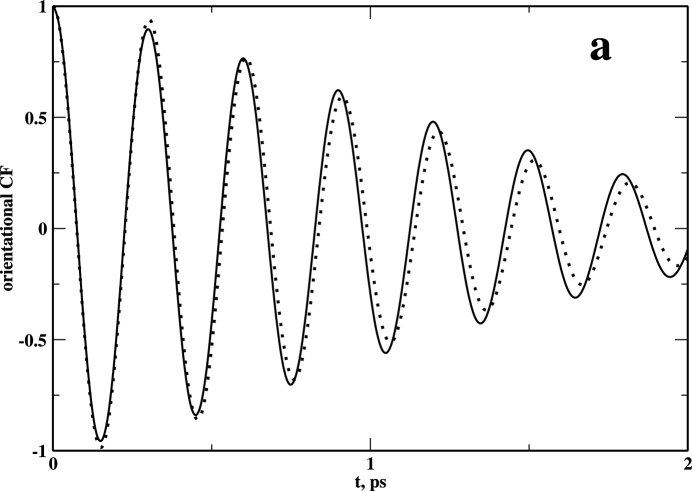
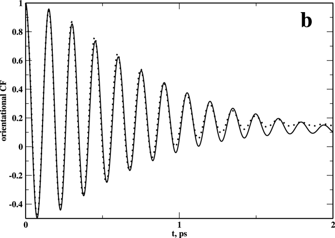
Figure 5: Orientational CFs of the first (a) and second (b) rank. Full lines depict the results of molecular dynamics simulations of CN fragments injected at the temperature $\overline{T}_{\Delta}=2875$ K into the heat bath of argon atoms at $T=120$ K (Refs. str06 ; str06a ), and dotted lines show the results of the calculations within the generalized J-diffusion model ($b=0.094$, $\nu=0.84$) with the initial $\delta$-distribution (19) centered at $\Delta=6.75$. For CN at $120$ K, $\tau_{r}=$$0.32$ ps.

Fig. 5 compares orientational CFs simulated for hot CN fragments injected at the temperature $\overline{T}_{\Delta}=2875$ K into the heat bath of argon atoms at $T=120$ K (Refs. str06 ; str06a ) and those calculated within the generalized J-diffusion model. The delta-function initial distribution (19) has been used in our calculations, since it corresponds to the procedure of the preparation of the ensemble of photofragments in the simulations. The simulated orientational CFs look qualitatively very similar to those described by Eq. (35). Quantitatively, they can be fitted by Eq. (35) relatively well, but the so-obtained decay rate of the second rank orientational CF turns out to be $1.4$ higher than that of the first rank CF. The orientational CFs which are exactly calculated within the generalized J-diffusion model are seen to reproduce the simulated CFs very well. This is remarkable, since we did not fit the simulated CFs: we used the parameters of the generalized J-diffusion model obtained in the previous Section through the comparison of the simulated and theoretical energy relaxation times. Namely, we took $b=0.094$, $\nu=0.84$, and $\Delta=6.75$. foot4 This lends an additional support to self-consistency and predictive strength of the generalized J-diffusion model.

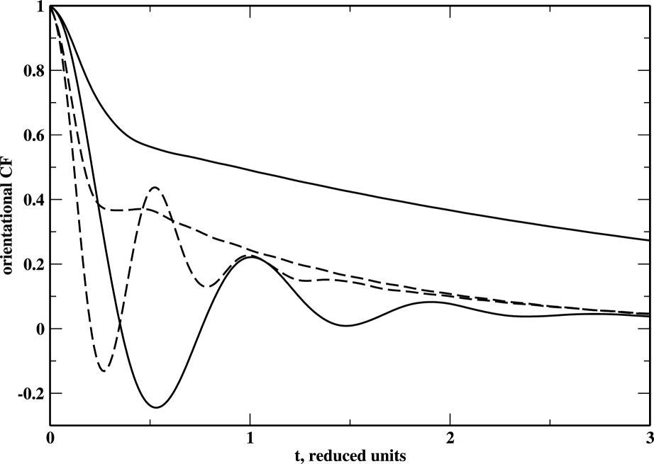
Figure 6: Orientational CFs of the first rank (full lines) and second rank (dashed lines) calculated for the “realistic values” of the model parameters ($\eta=1.1$, $\xi=1$, $\Delta=5.4$) and $\nu=7$. The upper lines correspond to the standard J-diffusion model ($b=0$) and the lower lines correspond to the generalized J-diffusion model ($b=0.1$).

Eq. (35) makes it clear that the persistence of the oscillatory behavior for orientational CFs is much higher in the generalized J-diffusion model, due to the $\Delta$-induced decrease of the relaxation rate, $\nu z(\Delta)$. This is vividly illustrated by Fig. 6, in which presented are the first and second rank orientational CFs calculated within the generalized ($b=0.1$) and standard ($b=0$) J-diffusion models for the “realistic values” of the model parameters ($\eta=1.1$, $\xi=1$, $\Delta=5.4$, and) and $\nu=7$ . The generalized J-diffusion model predicts the highly oscillatory orientational CFs. In exactly the same situation, the standard J-diffusion model predicts overdamped and slowly decaying CFs, which have nothing in common with the “true” CFs. Thus, the use of the standard (equilibrium) models of rotational relaxation beyond their domain of validity may lead to completely wrong predictions.

We can use Eq. (82) to derive a simple expression for orientational CFs in the case of strong dissipation, $\nu\gg 1$. As expected, they are described by the diffusion formula

$$G^{j}(t)=\exp\{-Dj(j+1)t\}$$ (36)

with the diffusion coefficient $D$ equaled to the equilibrium angular momentum integral relaxation time, $\tau_{J}^{eq}$. The latter is given by Eq. (74), so that

$$D=\tau_{J}^{eq}=\frac{1}{\nu(1-b)^{2}}.$$ (37)

The orientational relaxation times are calculated as

$$\tau_{\Omega}^{j}=\int_{0}^{\infty}dtG^{j}(t)=\widetilde{G}^{j}(0).$$ (38)

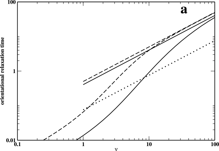
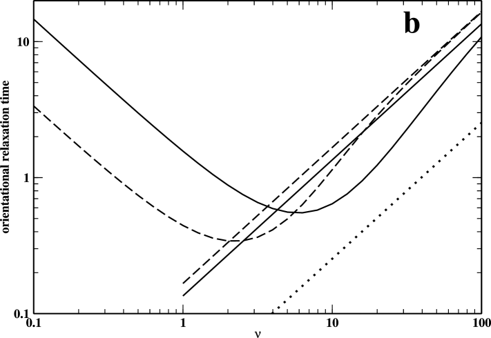
Figure 7: Orientational relaxation times $\tau_{\Omega}^{j}$ of the first (a) and second (b) rank vs. the collision rate $\nu$ calculated for the “realistic values” of the model parameters ($\eta=1.1$, $\xi=1$, $\Delta=5.4$). The dashed lines correspond to the $\tau_{\Omega}^{j}$ and modernized Hubbard asymptote $1/[j(j+1)\tau_{J}^{eq}]$ calculated within the standard J-diffusion model ($b=0$). The full lines correspond to their generalized J-diffusion model ($b=0.1$) counterparts. The standard Hubbard asymptotes, $1/[j(j+1)\tau_{J}],$ are depicted by dotted lines.

It is popular to plot these quantities vs. the angular momentum relaxation times or rates. BurTe ; Ric77 That is why Figs. 7 display the graphs $\tau_{\Omega}^{1}$ (a) and $\tau_{\Omega}^{2}$ (b) vs. $\nu$ calculated within the standard and generalized J-diffusion models.

To get a better idea about the behavior of these curves, it is insightful to obtain explicit expressions for $\tau_{\Omega}^{j}$ in case of weak and strong dissipation. If $\nu\ll 1$, then Eq. (82) predicts that $\tau_{\Omega}^{j}$ is inversely proportional to the rate $\nu$:

$$\tau_{\Omega}^{j}=\frac{c_{j}}{\nu}\left(\frac{\xi\eta}{\sqrt{(\eta-b)(\eta\xi^{2}-b)}}\exp\left\{\frac{\eta bE_{\Delta}}{(\eta-b)}\right\}+\frac{(1+b)c_{j}}{1-c_{j}}\right).$$ (39)

Here $c_{j}=a_{j0}/(2j+1)$ and $a_{j0}$ are explicitly given by Eq. (79). FootD The standard J-diffusion formula McCl77 ; BurTe is recovered at $b=0$. Again, if the product $bE_{\Delta}$ is $\sim 1$ or larger, then nonequilibrium initial conditions manifest themselves in a considerable increase of $\tau_{\Omega}^{2}$ in comparison with the standard J-diffusion predictions at $\nu<1$ (Figs. 7b).

When $\nu>1$, the situation changes and the standard J-diffusion model overestimates the actual values of $\tau_{\Omega}^{j}$ (Figs. 7). If $\nu\gg 1$ then the diffusion formula (36) holds and, therefore,

$$\tau_{\Omega}^{j}\tau_{J}^{eq}=\frac{1}{j(j+1)}.$$ (40)

This expression can be termed as the generalized Hubbard relation. The standard Hubbard relation, $\tau_{\Omega}^{j}\tau_{J}=[j(j+1)]^{-1}$, BurTe ; hub72 ; Ric77 is seen to be significantly off. This discrepancy is remarkable, since it embodies the breakdown of the linear response theory. Indeed, the onset of rotational diffusion occurs after the molecular angular momenta have been thermolized according to the bath-induced Boltzmann distribution (4). Thus the rotational diffusion equation (36) is a legitimate description at $t>\tau_{J}$ and the rotational diffusion coefficient is determined by the equilibrium rotational fluctuations and therefore by the equilibrium value of the angular momentum relaxation time, $\tau_{J}^{eq}$. As has been detailed in Section 4, if the system starts far from equilibrium, then its angular momentum relaxation time $\tau_{J}$ can differ dramatically from its equilibrium counterpart, $\tau_{J}^{eq}$. It is in this case we expect the breakdown of the linear response Green-Kubo-type formulas for transport coefficients, which identify the rotational diffusion coefficient $D$ with the angular momentum relaxation time $\tau_{J}$.

VI Conclusion

An adequate description of rotational and translational relaxation in liquids under nonequilibrium conditions (or within an interval of characteristic energies which highly exceeds that of the bath thermal energies) cannot be carried out in terms of conventional Langevin and Fokker-Planck equations with constant frictions or by master equations with constant relaxation rates: one has to take into account (linear and/or angular) velocity dependence of friction. gri84 ; str06 ; str06a ; kos06d ; kam ; mor74 ; zhu90 ; rob91 ; kos07 The present paper deals with studying nonequilibrium rotational and orientational relaxation. We have generalized the standard J-diffusion model by allowing its dissipation rate to be angular momentum dependent and calculated various nonequilibrium rotational and orientational CFs. The reaction $\mathrm{ICN}+h\nu\rightarrow\mathrm{CN+I}$ has been selected as a prototype process which produces highly nonequilibrium hot photofragments. We have used the results of computer simulations str06 ; str06a to obtain realistic values of the model parameters and to test our theoretical predictions.

We have found that nonequilibrium rotational relaxation rates assume the form $\nu\exp\left\{-bE_{\Delta}/(k_{B}T)\right\}$, where $\nu$ is the equilibrium rate, $E_{\Delta}$ is the initial “nonequilibrium energy”, $T$ is the equilibrium temperature of the heat bath, and $b$ is the dimensionless small parameter fixed for a system under study. Accordingly, the relaxation times have the Arrhenius energy dependence, $\nu^{-1}\exp\left\{bE_{\Delta}/(k_{B}T)\right\}$. So, there exist characteristic “nonequilibrium energy” $\overline{E}_{\Delta}\sim k_{B}T/b$ and “nonequilibrium temperature” $\overline{T}_{\Delta}\sim T/b$, starting from which the $J$-dependence of relaxation rate becomes important and induces a significant slowing of rotational relaxation. In agreement with simulations, str06 ; str06a relaxation of the rotational probability density is shown to be a bimodal time-dependent mixture of the initial nonequilibrium and final equilibrium distributions. The slowing of rotational relaxation induces a long lifetime of the initial nonequilibrium contribution, which manifests itself in pronounced coherent effects.

The slowing of rotational relaxation causes qualitative changes in molecular reorientation. In agreement with simulations, str06 ; str06a hot nonequilibrium molecules exhibit slightly perturbed coherent rotation, which persists for several rotational periods. A similar observation has recently been made in the context of molecular excitation by strong femtosecond pulses: nonequilibrium molecular wave packets can be formed in such a way as to slow their subsequent rotational relaxation. sei06

We have demonstrated that orientational CFs in the overdamped limit are described by the diffusion equation with the diffusion coefficient equaled to the equilibrium angular momentum integral relaxation time, $\tau_{J}^{eq}$. Thus the orientational relaxation times $\tau_{\Omega}^{j}$ obey the generalized Hubbard relation, $\tau_{\Omega}^{j}\tau_{J}^{eq}=[j(j+1)]^{-1}$. Since the nonequilibrium angular momentum relaxation time $\tau_{J}$ can differ substantially from its equilibrium counterpart $\tau_{J}^{eq}$, the standard Hubbard relation, BurTe ; hub72 ; Ric77 in which $\tau_{J}^{eq}$ is replaced by $\tau_{J}$, can be significantly off.

It should be emphasized that all rotational and orientational CFs and their relaxation times dependent explicitly on the nonequilibrium preparation of the molecular ensemble. This effect is unreproducible within the standard (equilibrium) rotational models, which predict that relaxation rates are independent of initial conditions and are given by the linear response theory. Thus, the Arrhenius forms of the rotational relaxation times, slowing down of rotational relaxation, and violation of the Hubbard relations are all manifestations of the breakdown of the linear response theory far from equilibrium.

In practical terms, the standard and generalized J-diffusion models are almost indistinguishable under equilibrium conditions. Under nonequilibrium conditions, their predictions differ dramatically. The differences are not only quantitative but, not infrequently, qualitative. The message is thus as follows: the friction and/or the relaxation rate must be taken $J$-dependent in order to adequately describe rotational relaxation far from equilibrium.

Note, finally, that our theory can straightforwardly be generalized to symmetric and asymmetric top molecules. In this latter case, the relaxation rate can be taken rotational energy dependent, rather than angular momentum dependent. The method of solution of the corresponding kinetic equations remains absolutely the same, and the explicit formulas for various CFs can be written down after a straightforward generalization of the results presented in the Appendixes. Our theory is also readily extendable to quantum case, by replacing the integrations over the angular momentum $J$ with summations over the rotational quantum number $j$, and switching from the classical orientational CFs (79) to their quantum mechanical counterparts (see, e.g., Ref. gel02 ). Such a generalization might be useful for describing rotational coherences and time-dependent alignments in nonequilibrium dissipative systems, like those studied in Ref. sei06

Appendix A Calculation of rotational CFs

Let $A(\mathbf{J})$ and $B(\mathbf{J})$ be arbitrary functions of the angular momentum. Then the CF

$$C_{AB}(t)=\left\langle A(\mathbf{J}(t))B(\mathbf{J})\right\rangle_{ne}$$ (41)

can be evaluated through the rotational kinetic equation (22) as follows:

$$C_{AB}(t)=\int d\mathbf{J}A(\mathbf{J})\rho(\mathbf{J},t),\,\,\,\rho(\mathbf{J},0)=\rho_{ne}(\mathbf{J})B(\mathbf{J}).$$ (42)

After applying the Laplace transform (1) to Eq. (22) with initial condition (42), we obtain

$$\widetilde{\rho}(\mathbf{J},s)=\frac{\rho_{ne}(\mathbf{J})B(\mathbf{J})+\nu(1+b)z(J)\rho_{B}(J)\widetilde{\sigma}(s)}{s+\nu z(J)}.$$ (43)

Here

$$\widetilde{\sigma}(s)\equiv\int d\mathbf{J}z(J)\widetilde{\rho}(\mathbf{J},s).$$ (44)

Multiplying Eq. (42) by $z(J)$ and integrating over $\mathbf{J}$, we obtain an algebraic equation for $\widetilde{\sigma}(s)$. Inserting its solution into Eq. (43), multiplying the so obtained expression by $A(\mathbf{J})$ and integrating over $\mathbf{J}$, we get

$$\widetilde{C}_{AB}(s)=\widetilde{\Phi}_{ne}(AB,s)+\nu(1+b)\frac{\widetilde{\Phi}_{B}(zA,s)\widetilde{\Phi}_{ne}(zB,s)}{1-\nu(1+b)\widetilde{\Phi}_{B}(z^{2},s)}.$$ (45)

Here we have introduced the functionals

$$\Phi_{a}(Y,t)=\int d\mathbf{J}\rho_{a}(\mathbf{J})\exp\{-\nu z(J)t\}Y(\mathbf{J}),\,\,\,\,\,a=B,\,ne$$ (46)

and their Laplace transforms

$$\widetilde{\Phi}_{a}(Y,s)=\int d\mathbf{J}\rho_{a}(\mathbf{J})\frac{Y(\mathbf{J})}{s+\nu z(J)},\,\,\,\,\,a=B,\,ne$$ (47)

which are defined for any function $Y(\mathbf{J})$.

In principle, Eq. (45) delivers the desirable expression for CF $\widetilde{C}_{AB}(s)$ which, after the numerical inversion of the Laplace transform, yields the CF in the time domain, $C_{AB}(t)$. The long-time limit of this CF is determined as follows:

$$C_{AB}(t\rightarrow\infty)\equiv\left\langle A\right\rangle_{B}\left\langle B\right\rangle_{ne}.$$ (48)

Here the averages are defined as

$$\left\langle Y\right\rangle_{a}\equiv\nu\widetilde{\Phi}_{a}(Yz,0)\equiv\int d\mathbf{J}\rho_{a}(\mathbf{J})Y(\mathbf{J}),\,\,\,\,a=B,\,ne.$$ (49)

If both $\left\langle A\right\rangle_{B}$ and $\left\langle B\right\rangle_{ne}$ are nonzero, then CF (41) possesses a stationary long-time asymptote (48). This is so for the rotational energy CF, for example. Therefore, $\widetilde{C}_{AB}(s)\rightarrow\left\langle A\right\rangle_{B}\left\langle B\right\rangle_{ne}/s$ when $s\rightarrow 0$. This is undesirable for doing numerics. It is more convenient to subtract this constant contribution and redefine the CF (41) as follows:

$$X_{AB}(t)\equiv\frac{C_{AB}(t)-\left\langle A\right\rangle_{B}\left\langle B\right\rangle_{ne}}{\left\langle AB\right\rangle_{ne}-\left\langle A\right\rangle_{B}\left\langle B\right\rangle_{ne}}.$$ (50)

Evidently, this CF is normalized to unity ($X_{AB}(0)=1$) and does not have any stationary asymptote ($X_{AB}(t)\rightarrow 0$ when $t\rightarrow\infty$).

Taking the Laplace transform of Eq. (50), we get

$$\widetilde{X}_{AB}(s)\equiv\frac{\widetilde{C}_{AB}(s)-\left\langle A\right\rangle_{B}\left\langle B\right\rangle_{ne}/s}{\left\langle AB\right\rangle_{ne}-\left\langle A\right\rangle_{B}\left\langle B\right\rangle_{ne}}.$$ (51)

Eq. (51) possesses yet an undesirable property: its numerator is a difference of two terms $\sim 1/s$. Of course, these two terms cancel each other when $s\rightarrow 0$ but it is convenient for numerical implementations to explicitly extract this singular contribution out of $\widetilde{C}_{AB}(s)$. To this end, we make use of the identity

$$\widetilde{\Phi}_{a}(Yz,s)\equiv\frac{1}{\nu}\left\{\left\langle Y\right\rangle_{a}-s\widetilde{\Phi}_{a}(Y,s)\right\},\,\,\,\,\,a=B,\,ne,$$ (52)

which is immediately derived from Eq. (47). Applying this formula several times, we can rewrite Eq. (51) in the following equivalent form

$$\widetilde{X}_{AB}(s)\equiv\frac{\widetilde{\Phi}_{ne}(AB,s)+\left(\nu\widetilde{\Phi}_{B}(z,s)\right)^{-1}\widetilde{\Psi}(s)}{\left\langle AB\right\rangle_{ne}-\left\langle A\right\rangle_{B}\left\langle B\right\rangle_{ne}}.$$ (53)

Here

$$\widetilde{\Psi}(s)\equiv\left\langle A\right\rangle_{B}\left\langle B\right\rangle_{ne}\widetilde{\Phi}_{B}(1,s)+s\widetilde{\Phi}_{B}(A,s)\widetilde{\Phi}_{ne}(B,s)-\left\langle A\right\rangle_{B}\widetilde{\Phi}_{ne}(B,s)-\left\langle B\right\rangle_{ne}\widetilde{\Phi}_{B}(A,s).$$ (54)

Eqs. (53) and (54) are our final singularity-free formulas, which are used for the numerical inversion of the Laplace transforms. The explicit formulas for CFs (23)-(25) can be obtained by inserting the corresponding functions $A(\mathbf{J})$ and $B(\mathbf{J})$ into Eqs. (53) and (54). For example, the angular momentum CF (23) corresponds to $A(\mathbf{J})=B(\mathbf{J})=\mathbf{J}$. Due to the isotropy of rotational space, $\widetilde{\Phi}_{a}(\mathbf{J}z^{n}(J),s)\equiv 0$, so that the general expression (53) simplifies considerably:

$$\widetilde{C}_{J}(s)=\frac{\widetilde{\Phi}_{ne}(E,s)}{\left\langle E\right\rangle_{ne}}.$$ (55)

There is no such a simplification for CFs (24) and (25), and all the terms (54) contribute into Eq. (53). We do not give the corresponding expressions explicitly, since they add nothing profound.

CF (50) can be used to define an important quantity, the integral relaxation time:

$$\tau_{AB}\equiv\int_{0}^{\infty}dtX_{AB}(t)\equiv\widetilde{X}_{AB}(0).$$ (56)

Since $\nu\widetilde{\Phi}_{B}(z,0)\equiv 1$, Eqs. (53) and (54) predict that

$$\tau_{AB}\equiv\frac{\widetilde{\Phi}_{ne}(AB,0)+\widetilde{\Psi}(0)}{\left\langle AB\right\rangle_{ne}-\left\langle A\right\rangle_{B}\left\langle B\right\rangle_{ne}}.$$ (57)

Here

$$\widetilde{\Psi}(0)\equiv\left\langle A\right\rangle_{B}\left\langle B\right\rangle_{ne}\widetilde{\Phi}_{B}(1,0)-\left\langle A\right\rangle_{B}\widetilde{\Phi}_{ne}(B,0)-\left\langle B\right\rangle_{ne}\widetilde{\Phi}_{B}(A,0).$$ (58)

If we assume that the relaxation rate is constant ($b=0,$ $z(J)=1$) then the J-diffusion model is recovered. In this case, evidently,

$$\widetilde{\Phi}_{a}(Y,s)=\frac{\left\langle Y\right\rangle_{a}}{s+\nu},\,\,\,\,\widetilde{\Phi}_{a}(Y,0)=\frac{\left\langle Y\right\rangle_{a}}{\nu},\,\,\,\,a=B,\,ne.$$

Then, Eqs. (53) and (57) simplify to

$$\widetilde{X}_{AB}(s)=\left(\nu+s\right)^{-1},\,\,\,X_{AB}(t)=\exp\{-\nu t\},\,\,\,\tau_{AB}=\left(\nu\right)^{-1}$$ (59)

irrespective of particular forms of $A(\mathbf{J})$, $B(\mathbf{J})$, and $\rho_{ne}(\mathbf{J})$. Thus all rotational CFs in the J-diffusion model decay exponentially with the rate $\nu$, and their integral relaxation times are all equaled to the inverse value of this rate.

If the relaxation rate is $J$-dependent ($b\neq 0$), the situation is much more complicated. However, the formulas simplify dramatically if the nonequilibrium distribution is given by the delta-function (19). If we assume, additionally, that $b\ll 1$ but the product $bE_{\Delta}$ can take any value, we can write then

$$\widetilde{\Phi}_{B}(Y,s)\approx\frac{\left\langle Y\right\rangle_{B}}{s+\nu},\,\,\,\,\widetilde{\Phi}_{ne}(Y,s)=\frac{\left\langle Y\right\rangle_{ne}}{s+\nu z(\Delta)}.$$

After the insertion of these expressions into Eqs. (53) and (54), we obtain

$$\widetilde{X}_{AB}(s)=\frac{1}{\nu z(\Delta)+s},\,\,\,X_{AB}(t)=\exp\{-\nu z(\Delta)t\},\,\,\,\tau_{AB}=\frac{1}{\nu z(\Delta)}$$ (60)

for any $A(\mathbf{J})$ and $B(\mathbf{J})$.

If we wish to follow how the initial nonequilibrium distribution $\rho_{ne}(\mathbf{J})$ transforms in time into the equilibrium one, $\rho_{B}(\mathbf{J})$, we must solve kinetic equation (22) with the initial condition $\rho(\mathbf{J},0)=\rho_{ne}(\mathbf{J})$. The solution is given by a slightly modified version of Eqs. (43) and (45):

$$\widetilde{\rho}(\mathbf{J},s)=\frac{\rho_{ne}(\mathbf{J})+\nu(1+b)z(J)\rho_{B}(\mathbf{J})\widetilde{\sigma}_{d}(s)}{s+\nu z(J)},$$ (61)

$$\widetilde{\sigma_{d}}(s)=\frac{\widetilde{\Phi}_{ne}(z,s)}{1-\nu(1+b)\widetilde{\Phi}_{B}(z^{2},s)}.$$ (62)

Appendix B Calculation of rotational integral relaxation times

If we employ the nonequilibrium initial distribution (17), then the quantities $\widetilde{\Phi}_{a}(Y,0)$ (Eq. (47)) can be evaluated analytically for any CF of interest in the present paper ($Y=1,\,E,\,E^{2}$). This means that the integral relaxation times $\tau_{AB}$ can also be calculated analytically. To this end, convenient is to introduce the generating function

$$\Upsilon(b)=\int JdJ\rho_{ne}(J)\exp\{b(J_{x}^{2}+J_{y}^{2})/2\}=$$

$$\frac{\xi\eta}{2\pi}\int dJ_{x}\int dJ_{x}\exp\{-\eta(J_{x}-\Delta)^{2}/2\}\exp\{-\eta(\xi J_{y})^{2}/2\}\exp\{b(J_{x}^{2}+J_{y}^{2})/2\}.$$ (63)

Evidently,

$$\widetilde{\Phi}_{ne}(E^{N},0)=\frac{1}{\nu}\frac{d^{N}\Upsilon(b)}{db^{N}},\,\,\,\,\widetilde{\Phi}_{B}(E^{N},0)=\widetilde{\Phi}_{ne}(E^{N},0)|_{\xi=\eta=1,\,\Delta=0};$$ (64)

$$\left\langle E^{N}\right\rangle_{a}=\nu\widetilde{\Phi}_{a}(E^{N},0)|_{b=0},\,\,\,\,a=B,\,ne.$$ (65)

Eq. (63) is elementary evaluated to yield

$$\Upsilon(b)=\frac{\xi\eta}{\sqrt{(\eta-b)(\eta\xi^{2}-b)}}\exp\left\{\frac{\eta b\Delta^{2}}{2(\eta-b)}\right\}.$$ (66)

Differentiating this expression with respect to $b$, we obtain:

$$\widetilde{\Phi}_{ne}(1,0)=\frac{1}{\nu}\Upsilon(b),$$ (67)

$$\widetilde{\Phi}_{ne}(E,0)=\frac{1}{\nu}\Upsilon(b)v(b),$$ (68)

$$\widetilde{\Phi}_{ne}(E^{2},0)=\frac{1}{\nu}\Upsilon(b)\left\{v^{2}(b)+w(b)\right\}.$$ (69)

Here

$$v(b)=\frac{1}{2}\left\{\frac{1}{\eta-b}+\frac{1}{\eta\xi^{2}-b}+\frac{(\eta\Delta)^{2}}{(\eta-b)^{2}}\right\},$$ (70)

$$w(b)=\frac{1}{2}\left\{\frac{1}{(\eta-b)^{2}}+\frac{1}{(\eta\xi^{2}-b)^{2}}+\frac{2(\eta\Delta)^{2}}{(\eta-b)^{3}}\right\}.$$ (71)

These expressions can be substituted into Eq. (57) to calculate various integral relaxation times. FootB In general, the so-obtained expressions are quite cumbersome and are not presented here. However, they are useful for obtaining simple elucidating formulas in several particular cases. If $b\ll\eta,\,\eta\xi^{2}$ and $\Delta\gg 1$, then

$$\Upsilon(b)\approx\exp\left\{\frac{b\Delta^{2}}{2}\right\},\,\,v(b)\approx\frac{\Delta^{2}}{2},\,\,w(b)\approx\frac{\Delta^{2}}{\eta}.$$ (72)

If the initial distribution (17) reduces to the equilibrium one ($\eta=\xi=1$, $\Delta=0$), we get

$$\Upsilon(b)=v(b)=\frac{1}{(1-b)},\,\,w(b)=\frac{1}{(1-b)^{2}}$$ (73)

and FootE

$$\tau_{J}^{eq}=\frac{1}{\nu(1-b)^{2}},\,\,\,\tau_{S}^{eq}=\tau_{E}^{eq}=\frac{1+b^{2}}{\nu(1-b)^{3}}>\tau_{J}^{eq}.$$ (74)

It has not escaped our notice that the integral relaxation times $\tau_{AB}$ (57) diverge for $b\geq\eta$, as predicted by Eqs. (66)-(71). Although such situation is far beyond the expected domain of validity of our model ($b\ll\eta$), there is nothing pathological in the occurrence of the “phase transition” at $b=\eta$ and all CFs are well behaved for $b\geq\eta$. This means simply that the $J$-dependence of relaxation rates slows rotational CFs so dramatically that their integral relaxation times do not exist.

Appendix C Calculation of orientational CFs

Having inserted the definition of orientational CF (34) into Eq. (13), we obtain the equation

$$\partial_{t}G^{j}(\mathbf{J},t)=-i\mathbf{J}\mathbf{L}^{j}G^{j}(\mathbf{J},t)-\nu z(J)G^{j}(\mathbf{J},t)$$

$$+\nu(1+b)z(J)\rho_{B}(\mathbf{J})\int d\mathbf{J}^{\prime}z(J^{\prime})G^{j}(\mathbf{J}^{\prime},t).$$ (75)

Here $L_{\alpha}^{j}$ are the matrix elements of the angular momentum operators $\hat{L}_{\alpha}$ over the D-functions: var89

$$(L_{x}^{j})_{kl}\pm i(L_{y}^{j})_{kl}=\delta_{k,l\mp 1}\{(j\pm l)(j\mp l+1)\}^{1/2},\,\,(L_{z}^{j})_{kl}=l\delta_{kl};\,\,-j\leq k,l\leq j.$$ (76)

Eq. (75) must be solved with the initial condition

$$G^{j}(\mathbf{J},t=0)=\rho_{ne}(\mathbf{J}).$$ (77)

Evidently,

$$G^{j}(t)\equiv\int d\mathbf{J}G^{j}(\mathbf{J},t).$$ (78)

Orientational CFs are calculated very similarly to rotational CFs (see Appendix A). First we introduce the free linear rotor orientational CF ste69

$$F^{j}(J,t)=a_{j0}+2\sum_{k=1}^{j}a_{jk}\cos\{kJt\},\,\,\,\,a_{jk}=\left(d_{0k}^{j}(\frac{\pi}{2})\right)^{2},$$ (79)

$d_{km}^{j}(\beta)$ being the reduced Wigner function. var89 We further define the functional

$$Q_{a}^{j}(Y,t)=\int d\mathbf{J}\rho_{a}(\mathbf{J})\exp\{-\nu z(J)t\}Y(\mathbf{J})F^{j}(J,t),\,\,\,\,\,a=B,\,ne$$ (80)

and its Laplace transform

$$\widetilde{Q}_{a}^{j}(Y,s)=\int d\mathbf{J}\rho_{a}(\mathbf{J})Y(\mathbf{J})\widetilde{F}^{j}(J,s+\nu z(J))=$$ (81)

$$\sum_{k=-j}^{j}a_{jk}\int d\mathbf{J}\rho_{a}(\mathbf{J})\frac{Y(\mathbf{J})}{s+\nu z(J)+ikJ},\,\,\,\,\,a=B,\,ne.$$

Then, closely following the derivation of Eq. (45), we obtain the following expression for the Laplace transform of the orientational CF:

$$\widetilde{G}^{j}(s)=\widetilde{Q}_{ne}^{j}(1,s)+\nu(1+b)\frac{\widetilde{Q}_{B}^{j}(z,s)\widetilde{Q}_{ne}^{j}(z,s)}{1-\nu(1+b)\widetilde{Q}_{B}^{j}(z^{2},s)}.$$ (82)

Since orientational CFs of dissipative molecules, as distinct from their bath-free counterparts (79) and rotational CFs (Appendix A), do not possess stationary asymptotes, this formula is well behaved in the limit $s\rightarrow 0$ and can be used for the numerical inversion of the Laplace images into the time domain.

- (1) U. Banin and S. Ruhman, J. Chem. Phys. 98, 4391 (1993).
- (2) E. Lenderink, K. Duppen, and D. A. Wiersma, Chem. Phys. Lett. 211, 503 (1993).
- (3) E. Lenderink, K. Duppen, F. P. X. Everdij, J. Marvi, R. Torre, and D. A. Wiersma, J. Phys. Chem. 100, 7822 (1996).
- (4) C. Wan, M. Gupta, and A. Zewail, Chem. Phys. Lett. 256, 279 (1996).
- (5) S. Gnanakaran, M. Lim, N. Pugliano, M. Volk, and R. M. Hochstrasser, J. Phys.: Condense Matter 8, 9201 (1996).
- (6) M. Volk, S. Gnanakaran, E. Gooding, Y. Kholodenko, N. Pugliano, and R. M. Hochstrasser, J. Phys. Chem. A. 101, 638 (1997).
- (7) M. Lim, S. Gnanakaran, and R. M. Hochstrasser, J. Chem. Phys. 106, 3485 (1997).
- (8) T. Kühne and P. Vöhringer, J. Phys. Chem. A 102, 4177 (1998).
- (9) S. Hess, H. Bürsing, and P. Vöhringer, J. Chem. Phys. 111, 5461 (1999).
- (10) M. Volk, J. Phys. Chem. A 103, 5621 (1999).
- (11) S. Hess, H. Hippler, T. Kühne, and P. Vöhringer, J. Phys. Chem. A 103, 5622 (1999).
- (12) H. Bürsing, J. Lindner, S. Hess, and P. Vöhringer, Appl. Phys. B. 71, 411 (2000).
- (13) H. Bürsing and P. Vöhringer, Phys. Chem. Chem. Phys. 2, 73 (2000).
- (14) H. Fidder, F. Tschirschwitz, O. Duhr, and E. T. J. Nibbering, J. Chem. Phys. 114, 6781 (2001).
- (15) A. C. Moskun and S. E. Bradforth, J. Chem. Phys. 119, 4500 (2003).
- (16) I. Benjamin and K. R. Wilson, J. Chem. Phys. 90, 4176 (1989).
- (17) I. I. Benjamin, U. Banin and S. Ruhman, J. Chem. Phys. 98, 8337 (1993).
- (18) I. Benjamin, J. Chem. Phys. 103, 2459 (1995).
- (19) N. Winter, I. Chorny, J. Vieceli and I. Benjamin, J. Chem. Phys. 119, 2127 (2003).
- (20) A. I. Krylov and B. B. Gerber, J. Chem. Phys. 100, 4242 (1994).
- (21) W. Coffey, M. Evans and P. Grigolini. Molecular Diffusion and Spectra (John Wiley & Sons, 1984). Chapters 7-9.
- (22) A. P. Blokhin and M. F. Gelin, Chem. Phys. 252, 323 (2000).
- (23) M. F. Gelin, J. Mol. Liq. 93, 51 (2001).
- (24) A. S. Moskun, A. E. Jailaubekov, S. E. Bradforth, G. Tao, and R. M. Stratt, Science 311, 1907 (2006).
- (25) G. Tao and R. M. Stratt, J. Chem. Phys. 125, 114501 (2006).
- (26) M. F. Gelin and D. S. Kosov, J. Chem. Phys. 125, 224502 (2006).
- (27) R. G. Gordon, J. Chem. Phys. 44, 1830 (1966).
- (28) M. Fixman and K. Rider, J. Chem. Phys. 51, 2425 (1969).
- (29) R. E. D. McClung, Adv. Mol. Rel. Int. Proc. 10, 83 (1977).
- (30) A. I. Burshtein and S. I. Temkin. Spectroscopy of Molecular Rotation in Gases and Liquids (Cambridge University Press, Cambridge, 1994).
- (31) R. A. Sack, Proc. Phys. Soc. B. 70, 402 (1957); ibid 70, 414 (1957).
- (32) M. F. Gelin and D. S. Kosov, J. Chem. Phys. 124, 144514 (2006).
- (33) P. S. Hubbard, Phys. Rev. A. 6, 2421 (1972).
- (34) G. W. Ford, J. T. Lewis and J. McConnell, Phys. Rev. A. 19, 907 (1979).
- (35) A. Morita, J. Chem. Phys. 76, 3198 (1982).
- (36) D. H. Lee and R. E. D. McClung, Chem. Phys. 112, 23 (1987).
- (37) J. S. Baskin and A. Zewail, J. Phys. Chem. 98, 3337 (1994).
- (38) J. S. Baskin and A. H. Zewail, J. Phys. Chem. A 105, 3680 (2001).
- (39) I. Nadler, D. Mahgerefteh, H. Reisler, and C. Wittig, J. Chem. Phys. 82, 3885 (1985).
- (40) Angular momentum dependent relaxation rates can be calculated for collisions of rigid nonspherical bodies, hoa71 ; fix72 ; mul93 but the so-obtained formulas are very cumbersome and the very use of the predictions of the gas-phase (uncorrelated binary collision) theories is questionable for our purposes.
- (41) M. R. Hoare, Adv. Chem. Phys. 20, 135 (1971).
- (42) K. L. Rider and M. Fixman, J. Chem. Phys. 57, 2548 (1972).
- (43) M. P. Allen, G. T. Evans, D. Frenkel, B. M. Mulder, Adv. Chem. Phys. 83, 89 (1993).
- (44) Gaussian expansions are commonly employed in quantum chemical calculations. We can also recall a similar factorized decomposition of the spectral density function in quantum relaxation theory. tan99
- (45) C. Meier and D. J. Tannor, J. Chem. Phys. 111, 3365 (1999).
- (46) A. P. Blokhin and M. F. Gelin, Phys. Chem. Chem. Phys. 4, 3356 (2002).
- (47) A. P. Blokhin, M. F. Gelin, I. I. Kalosha, S. A. Polubisok and V. A. Tolkachev, J. Chem. Phys. 110, 978 (1999).
- (48) In some cases, the effect of rotational predissociation on the anisotropy evolution can be taken into account as proposed in Ref. gel99
- (49) Note that the present parameter differs from its counterpart from Ref. gel02 by the factor of .
- (50) See discussion in supplementary material to Ref. str06 for a validity of using the gas phase distribution for the interpretation of condensed phase data.
- (51) Note that nonequilibrium CFs and simulated in str06 are also very similar.
- (52) D. A. Varshalovich, A. N. Moskalev and V. K. Hersonski. Quantum Theory of Angular Momentum (World Scientific, Singapore, 1989).
- (53) Since the C-N interatomic length has been taken as angstroms in, str06 ; str06a the free rotation period for CN at K is ps. If we recalculate the nonequilibrium temperature into the dimensionless transferred angular momentum, we get then . We used a slightly smaller vale of in our generalized J-diffusion calculations presented in Fig. 5, in order to better reproduce the oscillation period of the CFs.
- (54) J. G. Powles and G. Rickayzen, Mol. Phys. 33, 1207 (1977).
- (55) Note that for odd . Thus, if , then also for odd .
- (56) N. G. van Kampen, Stochastic Processes in Physics and Chemistry. (North-Holland, Amsterdam, 1992)
- (57) H. Mori, H. Fujisaka, and H. Shigematsu, Prog. Theor. Phys. 51, 109 (1974).
- (58) S.-B. Zhu, Phys. Rev. A 42, 3374 (1990).
- (59) S.-B. Zhu, S. Singh, J. Lee, and G. W. Robinson, Chem. Phys. 152, 221 (1991).
- (60) M. F. Gelin and D.S. Kosov. J. Chem. Phys. 126, 514721 (2007).
- (61) S. Ramakrishna and T. Seideman, J. Chem. Phys. 124, 034101 (2006).
- (62) The rotational Fokker-Planck equation with Gaussian friction gives very similar results (M. F. Gelin and D. S. Kosov, unpublished).
- (63) Strictly speaking, has uncertainty of the kind if we put in Eq. (24). If, however, we consider the limit of and when , then the quantities are well behaved.
- (64) A. G. St. Pierre and W. A. Steele, Phys. Rev. 184, 172 (1969).