Mott metal-insulator transition in the Hubbard model

Abstract

The Hubbard model in the strong-coupling regime is mainly studied by Kondo-lattice theory or $1/d$ expansion theory, with $d$ being the spatial dimensionality. In two dimensions and higher, the ground state within the Hilbert subspace with no order parameter is a normal Fermi liquid except for $n=1$ and $U/W=+\infty$, with $n$ being the electron density per unit cell, $U$ the on-site repulsion, and $W$ the bandwidth; the cooperation between the Kondo effect, which favors a local singlet on each unit cell, and a resonating-valence-bond effect, which favors a local singlet on each pair of nearest-neighbor unit cells, stabilizes the Fermi liquid, whose ground state is a singlet as a whole, in the strong-coupling regime. In the whole Hilbert space with no restriction, the normal Fermi liquid is unstable at least against a magnetic or superconducting state. This analysis confirms an early Fermi-liquid theory of high-temperature superconductivity, F. J. Ohkawa, Jpn. J. Appl. Phys. 26, L652 (1987). The ground state for $n=1$ and $U/W=+\infty$ is a Mott insulator. Actual metal-insulator transitions cannot be explained within the Hubbard model. In order to explain them, the electron-phonon interaction, multi-band or multi-orbital effects, and effects of disorder should be considered beyond the Hubbard model. The crossover between local-moment magnetism and itinerant-electron magnetism corresponds to that between a localized spin and a normal Fermi liquid in the Kondo effect and it is simply a Mott metal-insulator crossover.

I Introduction

The Mott metal-insulator (M-I) transition is an interesting and important issue in solid-state physics,mott and a lot of effort has been made towards clarifying it. tokura However, its theoretical treatment is still controversial. One of the most contentious issues is whether or not the transition can be explained within the Hubbard model.

In the Hubbard approximation, Hubbard1 ; Hubbard2 provided that the on-site repulsion $U$ is large enough such that $U\gtrsim W$ or $W/U\lesssim 1$, with $W$ being the bandwidth, a band splits into two subbands or the Hubbard gap opens between the upper Hubbard band (UHB) and the lower Hubbard band (LHB). In the Gutzwiller approximation, Gutzwiller1 ; Gutzwiller2 ; Gutzwiller3 a narrow band of quasi-particles appears around the chemical potential; the band and quasi-particles are called the Gutzwiller band and quasi-particles in this paper. One may speculate that the density of states in fact has a three-peak structure, with the Gutzwiller band between UHB and LHB. Both of the approximations are single-site approximations (SSA). Another SSA theory confirms this speculation, OhkawaSlave showing that the Gutzwiller band appears at the top of LHB when the electron density per unit cell $n$ is less than one, i.e., $n<1$. According to Kondo-lattice theory, Mapping-1 ; Mapping-2 ; Mapping-3 the three-peak structure corresponds to the Kondo peak between two subpeaks in the Anderson model, which is an effective Hamiltonian for the Kondo effect. An insulating state appears provided that not only the Hubbard gap opens but also the Fermi surface of the Gutzwiller quasi-particles vanishes.

Provided that $n=1$ and $W/U=+0$, an electron is localized at a unit cell and it behaves as a free localized spin, so that the ground state is infinitely degenerate and is a typical Mott insulator. This fact implies that the ground state is also a Mott insulator in the vicinity of $n=1$ and $W/U=+0$, as is also implied by experiment. However, there is an argument that contradicts this implication: For example, assume that a nonzero but infinitesimally small density of electrons are removed from the Mott insulator or holes are doped into the Mott insulator. It is reasonable that the holes are itinerant at $T=0$ K provided that no gap opens in the Gutzwiller band and no disorder exists.

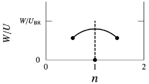
Figure 1: Schematic phase diagram of the ground state within the Hilbert subspace with no order parameter in two dimensions and higher. The ground state is a metal except for $n=1$ and $W/U=+0$. The arc indicates a possible but unlikely first-order transition line between metallic states, as is discussed in Sec. II.5. Dots indicate critical points. The dashed line indicates an insulator line implied by Brinkman and Rice’s theory, brinkman but it cannot survive when a resonating-valence -bond effect is considered, as is examined in Sec. III.2

In the Gutzwiller approximation, when $W/U=+0$ the effective mass of the quasi-particles diverges as $n\rightarrow 1\pm 0$. When $n\neq 1$, in fact, electrons are itinerant even for $W/U=+0$. According to Brinkman and Rice’s theory, brinkman which is also under the Gutzwiller approximation, when $n=1$ the effective mass diverges as $U\rightarrow U_{\rm BR}-0$, with $U_{\rm BR}\simeq W$. It is implied that, within the Hilbert subspace with no order parameter, the ground state is an insulator for $n=1$ and $0\leq W/U\leq W/U_{\rm BR}$, i.e., on the dashed line in the phase diagram shown in Fig. 1. The divergence of the effective mass occurs continuously, so that the M-I transition is of second order. It is unconventional that no order parameter appears in this second-order transition and no discontinuity seems to occur across the dashed line, which implies that the critical $U_{\rm BR}$ is infinite beyond the Gutzwiller approximation such that $W/U_{\rm BR}\rightarrow+0$.

One of the purposes of this paper is to show that no Mott M-I transition is possible at any finite $U$. Since actual M-I transitions cannot be explained within the Hubbard model, another purpose is to examine relevant effects for the transitions beyond the Hubbard model. The other purpose is to examine two issues related with the Mott M-I transition: the crossover between local-moment magnetism and itinerant-electron magnetism and high-temperature (high-$T_{c}$) superconductivity in cuprate oxides. bednortz This paper is organized as follows: The ground states within SSA and beyond SSA are studied in Secs. II and III, respectively. Relevant effects in actual M-I transitions are considered in Sec. IV. The magnetism crossover is considered in Sec. V. High-$T_{c}$ superconductivity is considered in Sec. VI. Discussion is given in Sec. VII. Conclusion is given in Sec. VIII. A proof of an inequality, which plays a critical role in this paper, is given in Appendix A. When cuprate oxide superconductors approach the Mott M-I transition or crossover, the specific heat coefficient $\gamma$ is suppressed loram ; momono and tunneling spectra are asymmetric, asymmetry1 both of which are unconventional. A phenomenological analysis on these issues is given in Appendix B.

II Fermi liquid within SSA

II.1 Fermi-surface condition

The Hubbard model is defined by

$${\cal H}=\epsilon_{a}\sum_{i\sigma}n_{i\sigma}-\sum_{i\neq j}\sum_{\sigma}t_{ij}a_{i\sigma}^{\dagger}a_{j\sigma}+U\sum_{i}n_{i\uparrow}n_{i\downarrow},$$ (1)

with $n_{i\sigma}=a_{i\sigma}^{\dagger}a_{i\sigma}$. The notations are conventional here. The dispersion relation of electrons is given by

$$E({\bf k})=\epsilon_{a}-\frac{1}{N}\sum_{i\neq j}t_{ij}\exp\left[i{\bf k}\cdot\left({\bf R}_{i}-{\bf R}_{j}\right)\right],$$ (2)

with $N$ being the number of unit cells and ${\bf R}_{i}$ the position of the $i$th lattice site. The density of states as a function of the electron energy $\varepsilon$ is defined by

$$\rho_{0}(\varepsilon)=\frac{1}{N}\sum_{\bf k}\delta[\varepsilon-E({\bf k})],$$ (3)

and, for convenience, the density of states as a function of the electron density $n$ is defined by

$$\bar{\rho}_{0}(n)=\frac{1}{N}\sum_{\bf k}\delta[\mu_{0}(n)-E({\bf k})],$$ (4a)

with $$\mu_{0}(n)$$ defined by

$$n=2\int_{-\infty}^{\mu_{0}(n)}d\varepsilon\rho_{0}(\varepsilon).$$ (4b)

An effective bandwidth of $E({\bf k})$ or $\rho_{0}(\varepsilon)$ is denoted by $W$ in this paper. It is assumed that the Fermi surface (FS) is present for $U=0$ or $\bar{\rho}_{0}(n)>0$ for any $0<n<2$.

As is discussed in Introduction, the Kondo effect has relevance to electron correlations in the Hubbard model. The $s$-$d$ model is one of the simplest effective Hamiltonians for the Kondo effect. According to Yosida’s perturbation theory yosida and Wilson’s renormalization-group theory, wilsonKG provided that FS of conduction electrons is present, the ground state of the $s$-$d$ model is a singlet or a normal Fermi liquid (FL) but is exceptionally a doublet for $J_{s\mbox{-}d}=0$, with $J_{s\mbox{-}d}$ the $s$-$d$ exchange interaction. The FL is stabilized by the Kondo effect or the quenching of magnetic moments by local quantum spin fluctuations.

The $s$-$d$ model is derived from the Anderson model, which is defined by

$${\cal H}_{A} = \sum_{{\bf k}\sigma}E_{c}({\bf k})c_{{\bf k}\sigma}^{\dagger}c_{{\bf k}\sigma}+\epsilon_{d}\sum_{\sigma}n_{d\sigma}+\tilde{U}n_{d\uparrow}n_{d\downarrow}$$ (5)

$$+\frac{1}{\sqrt{N_{A}}}\sum_{{\bf k}\sigma}\left[V({\bf k})c_{{\bf k}\sigma}^{\dagger}d_{\sigma}+(\mbox{h.c.})\right],$$

with $n_{d\sigma}=d_{\sigma}^{\dagger}d_{\sigma}$ and $N_{A}$ the number of unit cells. The notations are also conventional here. The hybridization energy is defined by

$$L_{\sigma}(i\varepsilon_{n})=\frac{1}{N_{A}}\sum_{\bf k}\frac{|V({\bf k})|^{2}}{i\varepsilon_{n}+\tilde{\mu}-E_{c}({\bf k})},$$ (6)

with $\tilde{\mu}$ being the chemical potential. It follows that

$$\mbox{Im}\left[L_{\sigma}(\varepsilon+i0)\right]=-\frac{\pi}{N_{A}}\sum_{\bf k}|V({\bf k})|^{2}\delta\left[\varepsilon+\tilde{\mu}-E_{c}({\bf k})\right],$$ (7)

A necessary and sufficient condition for the presence of FS is simply given by

$$\mbox{Im}\left[L_{\sigma}(+i0)\right]<0.$$ (8a)

When $$\mbox{Im}\left[L_{\sigma}(\varepsilon+i0)\right] \varepsilon=0$$ is discontinuous at ,

$$\lim_{\varepsilon\rightarrow\pm 0}\mbox{Im}\left[L_{\sigma}(\varepsilon+i0)\right]<0,$$ (8b)

is more relevant than Eq. (8a). The condition (8a) or (8b) is called the FS condition in this paper. According to the result on the $s$-$d$ model, yosida ; wilsonKG provided that the FS condition is satisfied, the ground state of the Anderson model is a singlet or a normal FL but is exceptionally a doublet for the just half filling and infinite $\tilde{U}$.

When there is no order parameter, the Green function of the Hubbard model is given by

$$G_{\sigma}(i\varepsilon_{n},{\bf k})=\frac{1}{i\varepsilon_{n}+\mu-E({\bf k})-\Sigma_{\sigma}(i\varepsilon_{n},{\bf k})},$$ (9)

with $\mu$ the chemical potential of the Hubbard model and $\Sigma_{\sigma}(i\varepsilon_{n},{\bf k})$ the single-particle self-energy. The self-energy is divided into single-site and multi-site self-energies:

$$\Sigma_{\sigma}(i\varepsilon_{n},{\bf k})=\tilde{\Sigma}_{\sigma}(i\varepsilon_{n})+\Delta\Sigma_{\sigma}(i\varepsilon_{n},{\bf k}).$$ (10)

Provided that the on-site interaction and the single-site electron lines are the same in the Feynman diagrams of the Hubbard and Anderson models, the single-site $\tilde{\Sigma}_{\sigma}(i\varepsilon_{n})$ is given by that of the Anderson model. The condition for the on-site interaction is simply given by $\tilde{U}=U$. The single-site Green function of the Hubbard model is given by

$$R_{\sigma}(i\varepsilon_{n})=\frac{1}{N}\sum_{\bf k}G_{\sigma}(i\varepsilon_{n}{\bf k}),$$ (11)

and that of the Anderson model is given by

$$\tilde{G}_{\sigma}(i\varepsilon_{n})=\frac{1}{\displaystyle i\varepsilon_{n}+\tilde{\mu}-\epsilon_{d}-\tilde{\Sigma}_{\sigma}(i\varepsilon_{n})-L_{\sigma}(i\varepsilon_{n})},$$ (12)

with $L_{\sigma}(i\varepsilon_{n})$ defined by Eq. (6). The condition for the electron lines is simply given by

$$R_{\sigma}(i\varepsilon_{n})=\tilde{G}_{\sigma}(i\varepsilon_{n}).$$ (13)

In fact, a set of $\tilde{U}=U$, $\tilde{\mu}-\epsilon_{d}=\mu-\epsilon_{a}$, and

$$L_{\sigma}(\varepsilon+i0)=\varepsilon+\mu-\epsilon_{a}-\tilde{\Sigma}_{\sigma}(\varepsilon+i0)-\frac{1}{R_{\sigma}(\varepsilon+i0)},$$ (14)

is a mapping condition to the Anderson model. A problem of calculating the single-site $\tilde{\Sigma}_{\sigma}(\varepsilon+i0)$ is reduced to a problem of determining and solving self-consistently the Anderson model. Mapping-1 ; Mapping-2 ; Mapping-3

When the multi-site $\Delta\Sigma_{\sigma}(i\varepsilon_{n},{\bf k})$ is ignored in the mapping condition (14), the approximation is the best SSA because it considers all the single-site terms. The SSA is rigorous for infinite dimensions within the Hilbert subspace with no order parameter. Metzner It can also be formulated as the dynamical mean-field theory georges ; RevMod ; kotliar ; PhyToday (DMFT) and the dynamical coherent potential approximation. dpca

II.2 Adiabatic continuation

The multi-site $\Delta\Sigma_{\sigma}(i\varepsilon_{n},{\bf k})$ is ignored in the following part of this section. Consider a Lorentzian model or the Hubbard model with a Lorentzian density of states:

$$\rho_{0}(\varepsilon)=\frac{1}{\pi}\frac{\Delta}{(\varepsilon-\epsilon_{a})^{2}+\Delta^{2}},$$ (15)

with $\Delta=W/\pi$. Then, Eq. (11) is simply given by

$$R_{\sigma}(\varepsilon+i0)=\frac{1}{\varepsilon+\mu-\epsilon_{a}+i\Delta-\tilde{\Sigma}_{\sigma}(\varepsilon+i0)}.$$ (16)

In principle, the mapping condition (14) should be treated in an iterative manner to determine the Anderson model to be solved. However, no iteration is needed for this model because Eq. (14) gives georges

$$L_{\sigma}(\varepsilon+i0)=-i\Delta,$$ (17)

even when any input $\tilde{\Sigma}_{\sigma}(\varepsilon+i0)$ is used in the right side of Eq. (14). The SSA is simply reduced to solving the Anderson model. Since the FS condition (8) is satisfied for the Anderson model, the ground state of the Hubbard model is a normal FL except for $n=1$ and $W/U=+0$.

One may argue that an M-I transition at finite $U$ is only possible when $\rho_{0}(\varepsilon)$ has finite band-tails. In order to examine a non-Lorentzian model of $\rho_{0}(\varepsilon)$, which may have finite or infinite band-tails, the following model is first examined:

$$\rho_{\delta}(\varepsilon)=-\frac{1}{\pi}\mbox{Im}\int d\varepsilon^{\prime}\frac{\rho_{0}(\varepsilon^{\prime})}{\varepsilon-\varepsilon^{\prime}+i\delta\Delta},$$ (18)

with $\delta>0$. In this non–Lorentzian model,

$$R_{\sigma}(\varepsilon+i0) = \int d\varepsilon^{\prime}\rho_{0}(\varepsilon^{\prime})$$ (19)

$$\times\frac{1}{\varepsilon+\mu-\epsilon_{a}-\varepsilon^{\prime}+i\delta\Delta-\tilde{\Sigma}_{\sigma}(\varepsilon+i0)},\qquad$$

instead of Eq. (16). As is proved in Appendix A,

$$\mbox{Im}L_{\sigma}(\varepsilon+i0)\leq-\delta\Delta,$$ (20)

for any input $\tilde{\Sigma}_{\sigma}(\varepsilon+i0)$. For example, one may argue a possible scenario for a Mott insulator with a nonzero gap across the chemical potential is that the self-energy develops a pole at $\varepsilon=0$ such that

$$\tilde{\Sigma}_{\sigma}(\varepsilon+i0)=c_{p}\frac{\Delta^{2}}{\varepsilon+i0}+\cdots,$$ (21)

with $c_{p}$ a numerical constant. Even if this type of the self-energy is tried as an input of the iterative process in order to search a self-consistent non-normal FL solution, $L_{\sigma}(\varepsilon+i0)$ given by the mapping condition (14) satisfies Eq. (20). Since the FS condition (8) is satisfied without fail in each iterative process to determine the Anderson model, no non-normal FL solution can be obtained in the SSA theory or the ground state of an eventual self-consistent SSA solution should be a normal FL. Provided that $\delta>0$, no M-I transition occurs at finite $U$. The ground state for $\rho_{\delta}(\varepsilon)$ with $\delta>0$ is a Mott insulator only at $n=1$ and $W/U=+0$.

An SSA solution for $\rho_{0}(\varepsilon)$ is obtained by the adiabatic continuation AndersonText of $\delta\rightarrow+0$. Provided that

$$\lim_{\varepsilon\rightarrow\pm 0}\lim_{\delta\rightarrow+0}\mbox{Im}L_{\sigma}(\varepsilon+i0)<0,$$ (22)

the ground state of the SSA solution is definitely a singlet or a normal FL. On the other hand, provided that

$$\lim_{\varepsilon\rightarrow\pm 0}\lim_{\delta\rightarrow+0}\mbox{Im}L_{\sigma}(\varepsilon+i0)=-0,$$ (23)

the ground state may be degenerate. The nature of the possible degeneracy is examined in Sec. II.4.

II.3 Fermi-liquid relation

First, consider the Anderson model self-consistently determined in the absence of any external field, and apply infinitesimally small Zeeman energy $g\mu_{B}H$ and chemical potential shift $\Delta\mu$ to the Anderson model; Weiss mean fields induced by the external fields are not included in this treatment. It is obvious that, provided that $\delta>0$, the adiabatic continuation AndersonText as a function of $U$ also holds. Therefore, the self-energy of the Anderson model for $\delta=+0$ is expanded in such a way that

$$\tilde{\Sigma}_{\sigma}(\varepsilon+i0) = \tilde{\Sigma}_{0}(0)+\left(1-\tilde{\phi}_{\gamma}\right)\varepsilon+\left(1-\tilde{\phi}_{s}\right)\frac{1}{2}\sigma g\mu_{B}H$$ (24)

$$+\left(1-\tilde{\phi}_{c}\right)\Delta\mu+O\left(\varepsilon^{2}\right),\qquad$$

at $T=0$ K, with $\tilde{\Sigma}_{0}(0)$, $\tilde{\phi}_{\gamma}$, $\tilde{\phi}_{s}$, and $\tilde{\phi}_{c}$ all being real. According to the Fermi-liquid relation,yosida-yamada the specific heat coefficient is given by

$$\gamma=\frac{2}{3}\pi^{2}k_{B}^{2}\tilde{\phi}_{\gamma}\rho^{*}(0).$$ (25)

Here, $\rho^{*}(0)$ or $\rho^{*}(\varepsilon)$ is the density of states defined by

$$\rho^{*}(\varepsilon)=-\frac{1}{\pi}\mbox{Im}\tilde{G}_{\sigma}(\varepsilon+i0)=-\frac{1}{\pi}\mbox{Im}R_{\sigma}(\varepsilon+i0).$$ (26)

Static spin and charge susceptibilities are given by

$$\tilde{\chi}_{s}(0)=2\tilde{\phi}_{s}\rho^{*}(0),$$ (27)

and

$$\tilde{\chi}_{c}(0)=2\tilde{\phi}_{c}\rho^{*}(0),$$ (28)

respectively. The conventional factor $(1/4)g^{2}\mu_{B}^{2}$ is not included in $\tilde{\chi}_{s}(0)$. It also follows that yosida-yamada

$$2\tilde{\phi}_{\gamma}=\tilde{\phi}_{s}+\tilde{\phi}_{c}.$$ (29)

Since the on-site $U$ is repulsive, local charge fluctuations are suppressed, so that

$$0<\tilde{\phi}_{c}/\tilde{\phi}_{\gamma}<1.$$ (30)

Then, it follows that

$$1<\tilde{\phi}_{s}/\tilde{\phi}_{\gamma}<2.$$ (31)

It is likely that $\tilde{\phi}_{c}/\tilde{\phi}_{\gamma}\ll 1$ and $\tilde{\phi}_{s}/\tilde{\phi}_{\gamma}\simeq 2$ for $n\simeq 1$ and $U/W\gtrsim 1$. The Kondo temperature, which is the energy scale of local quantum spin fluctuations, is defined by

$$k_{B}T_{K}=\left[1/\tilde{\chi}_{s}(0)\right]_{T=0~{}{\rm K}}.$$ (32)

The self-energy of the Hubbard model in the absence of any external field is simply given by $\tilde{\Sigma}_{\sigma}(\varepsilon+i0)$ with $g\mu_{B}H=0$ and $\Delta\mu=0$. The density of states for the Hubbard model is the same as that for the Anderson model model, as is shown in Eq. (26). According to the Fermi-liquid relation, Luttinger1 ; Luttinger2 the specific heat coefficient of the Hubbard model is also given by Eq. (25). Local spin and charge susceptibilities of the Hubbard model are given by Eqs. (27) and (28). The energy scale of local quantum spin fluctuations in the Hubbard model is also the Kondo temperature defined by Eq. (32).

According to the FS sum rule, Luttinger1 ; Luttinger2 the electron density $n$ is given by

$$n=\frac{1}{N}\sum_{{\bf k}\sigma}\theta\Bigl{(}[\mu-\epsilon_{a}-E({\bf k})-\tilde{\Sigma}_{0}(0)]/W\Bigr{)},$$ (33)

with $\theta(x)$ being the step function defined by

$$\theta(x)=\left\{\begin{array}[]{cc}0,&x<0\\ 1,&x>0\end{array}\right..$$ (34)

According to Eqs. (4) and (33), it follows that

$$\mu-\epsilon_{a}-\tilde{\Sigma}_{0}(0)=\mu_{0}(n).$$ (35)

According to Eq. (33) or (35), provided that $n$ is kept constant, $\mu-\tilde{\Sigma}_{0}(0)$, $R_{\sigma}(+i0)$, $\rho^{*}(0)$, and $L_{\sigma}(+i0)$ do not depend on $U$. It should be noted that

$$\rho^{*}(0) = \frac{1}{N}\sum_{{\bf k}\sigma}\delta\left[\mu-\epsilon_{a}-E({\bf k})-\tilde{\Sigma}_{0}(0)\right]$$ (36a)

$$= \bar{\rho}_{0}(n)>0,$$

and

$$\mbox{Im}L_{\sigma}(+i0)=-\frac{\pi\rho^{*}(0)}{\left[\mbox{Re}R_{\sigma}(+i0)\right]^{2}+\left[\pi\rho^{*}(0)\right]^{2}}<0.$$ (36b)

The dispersion relation and an effective bandwidth of the quasi-particles are defined, respectively, by

$$\xi_{0}({\bf k})=\frac{1}{\tilde{\phi}_{\gamma}}\left[\epsilon_{a}+E({\bf k})+\tilde{\Sigma}_{0}(0)-\mu\right],$$ (37)

and

$$W^{*}=W/\tilde{\phi}_{\gamma}.$$ (38)

The Green function (9) is approximately divided into the so called coherent and incoherent terms:

$$G_{\sigma}(i\varepsilon_{n},{\bf k})=\frac{1}{\tilde{\phi}_{\gamma}}\frac{1}{i\varepsilon_{n}-\xi_{0}({\bf k})}+[\mbox{incoherent term}].$$ (39)

Here, the first term is the coherent term, which describes the quasi-particle band, and the incoherent term describes LHB and UHB.

II.4 Possible degeneracy

Equation (36b) shows that the FS condition (8a) is satisfied by the SSA solution for $\delta=+0$, as is expected. When both of $\rho_{0}(\varepsilon)$ and $\tilde{\Sigma}_{\sigma}(\varepsilon+i0)$ are continuous and finite, $L_{\sigma}(\varepsilon+i0)$ is continuous so that the FS condition (8b) is also satisfied. In such a case, the ground state is never degenerate and is simply a normal FL. On the other hand, when $\rho_{0}(\varepsilon)$ or $\tilde{\Sigma}_{\sigma}(\varepsilon+i0)$ is discontinuous or divergent, $L_{\sigma}(\varepsilon+i0)$ can be discontinuous so that it is possible that the FS condition (8b) is not satisfied or Eq. (23) is satisfied, Eq. (36b) notwithstanding.

When $\rho_{0}(\varepsilon)$ is discontinuous or divergent at $\varepsilon=\mu_{0}(n)$, $\mbox{Re}R_{\sigma}(\varepsilon+i0)$ or $\rho^{*}(\varepsilon)$ is divergent at $\varepsilon=0$. Then, Eq. (23) is satisfied so that the ground state may be degenerate. When $\rho_{0}(\varepsilon)$ is divergent at $\varepsilon=\mu_{0}(n)$, the ground state is degenerate even for $U=0$.

Since $\tilde{\phi}_{\gamma}$ is finite in Eq. (24) provided that $\delta>0$, only the possible scenario for the discontinuity or divergence of $\tilde{\Sigma}_{\sigma}(\varepsilon+i0)$ at $\varepsilon=0$ is that $\tilde{\phi}_{\gamma}\rightarrow+\infty$ as $\delta\rightarrow+0$. In such a case, the real part of $\tilde{\Sigma}_{\sigma}(\varepsilon+i0)$ is at least discontinuous at $\varepsilon=0$; it may be finite or divergent as $\varepsilon\rightarrow\pm 0$. When the real part is discontinuous, the imaginary part exhibits logarithmic divergences as $\varepsilon\rightarrow\pm 0$ according to the Kramers-Kronig relation. Provided that $\tilde{\phi}_{\gamma}\rightarrow+\infty$ as $\delta\rightarrow+0$, it follows that

$$\lim_{\varepsilon\rightarrow\pm 0}\lim_{\delta\rightarrow+0}\rho^{*}(\varepsilon)=+0,$$ (40a)

and

$$\lim_{\varepsilon\rightarrow\pm 0}\lim_{\delta\rightarrow+0}\mbox{Im}L_{\sigma}(\varepsilon+i0)=-0.$$ (40b)

It should be noted that Eq. (36), which is for $\varepsilon=0$, still holds. In the exceptional case of $n=1$ and $W/U=+0$,

$$\rho^{*}(\varepsilon)=0,$$ (41a)

and

$$\mbox{Im}L_{\sigma}(\varepsilon+i0)=0,$$ (41b)

for any finite $\varepsilon$, and for any $\delta\geq+0$.

There are three possible scenarios for the phase diagram: When the divergence of $\tilde{\phi}_{\gamma}$ occurs as $\delta\rightarrow+0$ at a point on the $\delta=0$ plane, the point is a critical point. When it occurs as $\delta\rightarrow+0$ at any point on a line, the line is a critical line. When it occurs as $\delta\rightarrow+0$ at any point on a plane, the plane is a critical plane. The transition is of second order in any scenario.

It is unlikely that there is an isolated critical point of $n\neq 1$ or $W/U>+0$. When the scenario of a critical point is the case, the critical point should be the point of $n=1$ and $W/U=+0$. The critical point is exotic because there is discontinuity in $\rho^{*}(\varepsilon)$ as a function of $\varepsilon$, $n$, and $W/U$ at the critical point, as is shown in Eqs. (36), (40), and (41). The critical line and plane on the $\delta=0$ plane are more exotic than the critical point is. They should include the point of $n=1$ and $W/U=+0$ as a critical point within themselves. Then, there is discontinuity in $\rho^{*}(\varepsilon)$ as a function of $\varepsilon$, $n$, and $W/U$ at the critical point even within the critical line and plane.

According to Eqs. (25), (31), and (32), $\gamma\rightarrow+\infty$  mJ/mol K² and $T_{K}\rightarrow+0$ K as $\tilde{\phi}_{\gamma}\rightarrow+\infty$, which simply means that low-energy or zero-energy states are accumulated or the ground state is degenerate. The divergence of the local spin susceptibility $\tilde{\chi}_{s}(0)$ is also one of the consequences of the degeneracy of the ground state. At the critical point of $n=1$ and $W/U=+0$, an electron behaves as a free localized spin so that $\tilde{\chi}_{s}(0)=1/k_{B}T$, which diverges as $T\rightarrow 0$ K. A similar divergent behavior is expected on the critical line or plane.

In a conventional second-order phase transition, not only an order parameter and infinite degeneracy of the ground state but also rigidity appear so that a ground-state configuration is rigidly realized among infinitely degenerate ones; the Nambu-Goldstone mode appears and the entropy is zero at $T=0$ K. Only an external field conjugate to the order parameter can lift the degeneracy of the ground state. The transition discussed here, which is also of second order, is quite different from the conventional one. No order parameter or no rigidity appears so that the Nambu-Goldstone mode does not appear and the entropy is nonzero at $T=0$ K, i.e., the third law of thermodynamics does not hold. An infinitesimally small perturbation such as $\delta=+0$ can easily lift the degeneracy or the degenerate ground state is not rigid against an infinitesimally small perturbation. These unconventional features are totally obvious or trivial for the critical point of $n=1$ and $W/U=+0$.

When the ground state is degenerate, rigorously speaking, the FL is not a normal FL. However, since Eq. (36a) is satisfied even for $\delta=+0$ and no order parameter or no rigidity appears, an SSA solution with $T_{K}=+0$ K can be regarded as a normal FL with a vanishing effective Fermi energy. In fact, if $\tilde{\phi}_{\gamma}$ is extremely large but is still finite for an extremely small but nonzero $\delta$, an SSA solution for such a small $\delta$ is a normal FL with an extremely small but nonzero Fermi energy.

In the Gutzwiller approximation, Gutzwiller1 ; Gutzwiller2 ; Gutzwiller3 when $W/U=+0$ it follows that $\tilde{\phi}_{\gamma}\propto 1/|1-n|$, which implies that the scenario of a critical plane is unlikely. Then, Brinkman and Rice’s theory brinkman implies the existence of the critical line of $n=1$ and $0\leq W/U\leq W/U_{\rm BR}$, as is discussed in Introduction; it is obvious that no discontinuity can occur across the critical line. The degenerate ground state on the critical line is not rigid, as is discussed above. It is therefore speculated that, provided that $\rho_{0}(\varepsilon)$ is continuous and finite at $\varepsilon=\mu_{0}(n)$, the critical line cannot survive in an SSA beyond the Gutzwiller approximation; it cannot survive beyond SSA, as is examined in Sec. III.2.

II.5 Possible first-order metal-metal transition

It is assumed so far that a self-consistent SSA solution is unique. If it is not unique, a first-order transition between metallic states is possible. However, the adiabatic continuation still holds, for example, along a route around one of the critical points at the ends of the first-order transition line. Consider two metallic states that are on different sides of the line but are infinitesimally close to each other. Since $n$’s are the same in two metallic states, the FS sum rule, $\rho^{*}(0)$, and $L_{\sigma}(+i0)$ are all the same in the two metallic states. It is difficult to imagine that, for example, $\tilde{\phi}_{\gamma}$ shows a jump across the line. The occurrence of such a first-order transition is unlikely. The transition never occurs in the Lorentzian model because the mapping is unique. The transition line is shown on a schematic phase diagram in Fig. 1, although it is unlikely.

III Ground state beyond SSA

III.1 Kondo-lattice or $1/d$ expansion theory

The irreducible spin polarization function is also divided into single-site and multi-site functions:

$$\pi_{s}(i\omega_{l},{\bf q})=\tilde{\pi}_{s}(i\omega_{l})+\Delta\pi_{s}(i\omega_{l},{\bf q}).$$ (42)

The single-site $\tilde{\pi}_{s}(i\omega_{l})$ is given by that of the Anderson model. The spin susceptibilities of the Anderson and Hubbard models are given, respectively, by

$$\tilde{\chi}_{s}(i\omega_{l})=\frac{2\tilde{\pi}_{s}(i\omega_{l})}{1-U\tilde{\pi}_{s}(i\omega_{l})},$$ (43)

and

$$\chi_{s}(i\omega_{l},{\bf q})=\frac{2\pi_{s}(i\omega_{l},{\bf q})}{1-U\pi_{s}(i\omega_{l},{\bf q})}.$$ (44)

A physical picture for Kondo lattices is that local spin fluctuations on different sites interact with each other by an intersite exchange interaction. In Kondo-lattice theory, according to this physical picture, an intersite exchange interaction $I_{s}(i\omega_{l},{\bf q})$ is defined by

$$\chi_{s}(i\omega_{l},{\bf q})=\frac{\tilde{\chi}_{s}(i\omega_{l})}{1-\frac{1}{4}I_{s}(i\omega_{l},{\bf q})\tilde{\chi}_{s}(i\omega_{l})}.$$ (45)

Provided that $U/W\gtrsim 1$, it follows that

$$I_{s}(i\omega_{l},{\bf q})=2U^{2}\Delta\pi_{s}(i\omega_{l},{\bf q})\left[1+O\left(\frac{1}{U\tilde{\chi}_{s}(i\omega_{l})}\right)\right],$$ (46)

where terms of $O[1/U\tilde{\chi}_{s}(i\omega_{l})]$ can be ignored. The strong coupling case of $U/W\gtrsim 1$ is mainly studied in this section.

The exchange interaction $I_{s}(i\omega_{l},{\bf q})$ is composed of three terms: three-exchange ; itinerant-ferro

$$I_{s}(i\omega_{l},{\bf q})=J_{s}({\bf q})+J_{Q}(i\omega_{l},{\bf q})-4\Lambda(i\omega_{l},{\bf q}).$$ (47)

The first term $J_{s}({\bf q})$ is the superexchange interaction. According to field theory, it arises from the exchange of a pair excitation of electrons between LHB and UHB. sup-exchange When the widths of LHB and UHB are vanishingly small, the strength of the superexchange interaction between nearest neighbors is $J=-4|t|^{2}/U$, with $t$ the transfer integral between nearest neighbors. Since the widths of LHB and UHB are nonzero, $|J|$ becomes substantially smaller than $4|t|^{2}/U$, for example, about a half of $4|t|^{2}/U$ in a realistic condition. exchange-reduction

The second term $J_{Q}(i\omega_{l},{\bf q})$ is an exchange interaction arising from the exchange of a pair excitation of the quasi-particles. According to the Ward relation, ward the static component of the single-site irreducible three-point vertex function in spin channels is given by

$$\tilde{\lambda}_{s} = \tilde{\phi}_{s}[1-U\tilde{\pi}_{s}(0)]$$ (48)

$$= \frac{2\tilde{\phi}_{s}}{U\tilde{\chi}_{s}(0)}\left[1+O\left(\frac{1}{U\tilde{\chi}_{s}(0)}\right)\right],$$

where terms of $O[1/U\tilde{\chi}_{s}(0)]$ can also be ignored. When only the coherent part of the Green function is considered and this $\tilde{\lambda}_{s}$ is approximately used for low-energy dynamical processes, $J_{Q}(i\omega_{l},{\bf q})$ is given by

$$J_{Q}(i\omega_{l},{\bf q})=P(i\omega_{l},{\bf q})-\frac{1}{N}\sum_{\bf q}P(i\omega_{l},{\bf q}),$$ (49)

with

$$P(i\omega_{l},{\bf q}) = \frac{4}{\tilde{\chi}_{s}^{2}(0)}\left(\frac{\tilde{\phi}_{s}}{\tilde{\phi}_{\gamma}}\right)^{2}$$ (50)

$$\times\frac{1}{N}\sum_{{\bf k}\sigma}\frac{f[\xi_{0}({\bf k})]-f[\xi_{0}({\bf k}+{\bf q})]}{i\omega_{l}-\xi_{0}({\bf k}+{\bf q})+\xi_{0}({\bf k})},\qquad$$

with $f(\varepsilon)=1/[e^{\varepsilon/k_{B}T}+1]$. In Eq. (49), the single-site term is subtracted because it is considered in SSA. The strength of this exchange interaction is proportional to $1/\tilde{\chi}_{s}(0)=k_{B}T_{K}$, which is proportional to the quasi-particle bandwidth.satoh1 ; satoh2 It is antiferromagnetic when the nesting of FS is sharp or the chemical potential lies around the center of the quasi-particle band. It is ferromagnetic when the chemical potential lies around the top or bottom of the quasi-particle band. In particular, it is strongly ferromagnetic when the density of states has a sharp peak at one of the band edges where chemical potential lies, itinerant-ferro ; satoh1 ; satoh2 ; miyai as it has a sharp peak in many itinerant-electron ferromagnets such as Fe, Ni, and so on.

The third term $-4\Lambda(i\omega_{l},{\bf q})$ corresponds to the mode-mode coupling term of spin fluctuations in the self-consistent renormalization (SCR) theory, moriya which is relevant for $U/W\lesssim 1$.

When the three-point vertex function $\tilde{\lambda}_{s}$ given by Eq. (48) is approximately used for low-energy dynamical processes, the mutual interaction between the quasi-particles is given by

$$\frac{1}{4}(U\tilde{\lambda}_{s})^{2}[\chi_{s}(i\omega_{l},{\bf q})-\tilde{\chi}_{s}(i\omega_{l})]=\frac{1}{4}\tilde{\phi}_{s}^{2}I_{s}^{*}(i\omega_{l},{\bf q}),$$ (51)

with

$$I_{s}^{*}(i\omega_{l},{\bf q})=\frac{I_{s}(i\omega_{l},{\bf q})}{1-\frac{1}{4}I_{s}(i\omega_{l},{\bf q})\tilde{\chi}_{s}(i\omega_{l})}.$$ (52)

In Eq. (51), the single-site term is subtracted because it is considered in SSA, and two $\tilde{\phi}_{s}$ appear as effective three-point vertex functions. It should be noted that the mutual interaction mediated by spin fluctuations is essentially the same as that due to the exchange interaction $I_{s}(i\omega_{l},{\bf q})$ or $I_{s}^{*}(i\omega_{l},{\bf q})$.

In Kondo-lattice theory, an unperturbed state is constructed in the non-perturbative SSA theory and intersite effects are perturbatively considered in terms of $I_{s}(i\omega_{l},{\bf q})$ or $I_{s}^{*}(i\omega_{l},{\bf q})$. Kondo-lattice theory can also be formulated as $1/d$ expansion theory,Mapping-2 ; Mapping-3 with $d$ the spatial dimensionality. What remain nonzero in the limit of $d\rightarrow+\infty$ are the single-site self-energy $\tilde{\Sigma}_{\sigma}(i\varepsilon)$, the single-site polarization function $\tilde{\chi}_{s}(i\omega_{l})$, and the magnetic exchange interactions, $J_{s}({\bf Q})$ and $J_{Q}(i\omega_{l},{\bf Q})$, for particular ${\bf Q}$’s in the Brillouin zone; both of $J_{s}({\bf q})$ and $J_{Q}(i\omega_{l},{\bf q})$ vanish for almost all ${\bf q}$’s. When the Néel temperature $T_{N}$ is nonzero, magnetization ${\bf m}({\bf Q})$ appears at $T<T_{N}$. Therefore, $J_{s}({\bf Q}){\bf m}({\bf Q})$ and $J_{Q}(i\omega_{l},{\bf Q}){\bf m}({\bf Q})$ can be nonzero even in the limit of $d\rightarrow+\infty$, which are Weiss mean fields. All the other terms such as $\Delta\Sigma_{\sigma}(i\varepsilon_{n},{\bf k})$ and $-4\Lambda(i\omega_{l},{\bf q})$ vanish in the limit of $d\rightarrow+\infty$. com1/D

III.2 Stabilization of the normal Fermi liquid

The quasi-particles are renormalized by the intersite exchange interaction $I_{s}^{*}(i\omega_{l},{\bf q})$. One of the main terms of $I_{s}^{*}(i\omega_{l},{\bf q})$ is the superexchange interaction:

$$I_{s}^{*}(i\omega_{l},{\bf q}) = I_{s}(i\omega_{l},{\bf q})+\frac{\frac{1}{4}I_{s}^{2}(i\omega_{l},{\bf q})\tilde{\chi}_{s}(i\omega_{l})}{1-\frac{1}{4}I_{s}(i\omega_{l},{\bf q})\tilde{\chi}_{s}(i\omega_{l})}$$ (53)

$$= J_{s}({\bf q})+J_{Q}(i\omega_{l},{\bf q})+\cdots.$$

There are two types of the renormalization linear in the superexchange interaction. One is a Hartree-type term,mag-structure $\tilde{\phi}_{s}J_{s}({\bf Q}){\bm{m}}({\bf Q})$, which may cause magnetic instability. In this subsection, it is not considered in order to restrict the Hilbert space within the subspace with no order parameter; possible instabilities are examined in Sec. III.3. The other is a Fock-type term, which stabilizes the FL, as is examined below.

When only the coherent term of the Green function is considered, the Fock-type term is given bycomFullSelfconsistet

$$\Delta\Sigma_{\sigma}({\bf k})=\frac{3}{4}\frac{\tilde{\phi}_{\rm s}^{2}}{\tilde{\phi}_{\gamma}}\frac{k_{B}T}{N}\sum_{\varepsilon_{n^{\prime}}{\bf k}^{\prime}}J_{s}({\bf k}-{\bf k}^{\prime})\frac{e^{i\varepsilon_{n^{\prime}}0^{+}}}{i\varepsilon_{n}^{\prime}-\xi_{0}({\bf k}^{\prime})}.$$ (54)

Here, the factor 3 appears because of three spin channels and two effective vertex functions $\tilde{\phi}_{\rm s}^{2}$ appear. When the multi-site self-energy is considered in the mapping condition (14), the single-site and multi-site terms depend on each other. In principle, therefore, they should also be self-consistently calculated with each other. Once $\tilde{\phi}_{\gamma}$, $\tilde{\phi}_{s}$, and $\Delta\Sigma_{\sigma}({\bf k})$ are self-consistently calculated, the dispersion relation of the quasi-particles is given by

$$\xi({\bf k})=\frac{1}{\tilde{\phi}_{\gamma}}\left[\epsilon_{a}+E({\bf k})+\tilde{\Sigma}_{0}(0)+\Delta\Sigma_{\sigma}({\bf k})-\mu\right],$$ (55)

and the density of states at the chemical potential by

$$\rho^{*}(0)=\frac{1}{N}\sum_{\bf k}\delta\left[\epsilon_{a}+E({\bf k})+\tilde{\Sigma}_{0}(0)+\Delta\Sigma_{\sigma}({\bf k})-\mu\right].$$ (56)

When this $\rho^{*}(0)$ is used instead of Eq. (36a), the specific heat coefficient is given by Eq. (25) and the local spin susceptibility is given by Eq. (27)

The renormalization (54) depends on dimensionality $d$ and the lattice structure. When only the superexchange interaction $J$ between nearest neighbors is considered, for example, in a square-lattice model, it follows that

$$\frac{1}{\tilde{\phi}_{\gamma}}\Delta\Sigma_{\sigma}({\bf k})=\frac{3}{4}\left(\frac{\tilde{\phi}_{\rm s}}{\tilde{\phi}_{\gamma}}\right)^{2}J\Xi\left[\cos(k_{x}a)+\cos(k_{y}a)\right],$$ (57)

with $a$ the lattice constant, and

$$\Xi=\frac{1}{N}\sum_{{\bf k}}\theta\left[-\frac{\xi_{0}({\bf k})}{W}\right]\left[\cos(k_{x}a)+\cos(k_{y}a)\right].$$ (58)

Since $1<\tilde{\phi}_{s}/\tilde{\phi}_{\gamma}<2$, as is shown in Eq. (31), Eq. (57) remains nonzero even if $\tilde{\phi}_{\gamma}$ is divergent. In general, when an effective bandwidth of $\Delta\Sigma_{\sigma}({\bf k})/\tilde{\phi}_{\gamma}$ is denoted by $c_{J}|J|$, an effective bandwidth of $\xi({\bf k})$ is given by

$$W^{*}=\frac{W}{\tilde{\phi}_{\gamma}}+c_{J}|J|,$$ (59)

with $c_{J}=O(1)$ being a numerical constant, which depends on $d$ and the lattice structure.

When this renormalization is considered, it follows that

$$\rho^{*}(0)\simeq\frac{1}{\displaystyle W+\tilde{\phi}_{\gamma}c_{J}|J|},$$ (60)

and

$$k_{B}T_{K}=\frac{1}{2\tilde{\phi}_{s}\rho^{*}(0)}\simeq\frac{\displaystyle W+\tilde{\phi}_{\gamma}c_{J}|J|}{2\tilde{\phi}_{s}}.$$ (61)

It should be noted that the Kondo temperature $T_{K}$ is nonzero even if $\tilde{\phi}_{s}\rightarrow+\infty$ or $\tilde{\phi}_{\gamma}\rightarrow+\infty$, provided that $|J|$ is nonzero. Since the vanishment of $T_{K}$ and the divergence of $\tilde{\phi}_{\gamma}$ occur together in any case provided that the ground state is degenerate, the fact that $T_{K}$ can never be zero leads to a conclusion that the divergence of $\tilde{\phi}_{\gamma}$ can never occur provided that $\tilde{\phi}_{\gamma}$ is self-consistently calculated beyond SSA. The degeneracy of the ground state never occurs except for $n\rightarrow 1$ and $W/U\rightarrow+0$. Even if the critical line or plane is present under SSA, it can never survive beyond SSA. It is trivial that the critical point $n=1$ and $W/U=+0$ survives.

It follows according to Eq. (60) that

$$\lim_{\tilde{\phi}_{\gamma}\rightarrow+\infty}\rho^{*}(0)=+0,$$ (62)

for $|J|\neq 0$ or $W/U>0$. Excepting on the line of $W/U=+0$, there is no discontinuity in $\rho^{*}(\varepsilon)$ as a function of $\varepsilon$, $n$, and $W/U$. However, there is still a discontinuity at $n=1$ on the line of $W/U=+0$. This discontinuity presumably vanishes when the renormalization by the total $I_{s}^{*}(i\omega_{l},{\bf q})$ is considered. The critical point of $n=1$ and $W/U=+0$ is a conventional one beyond SSA.

When the superexchange interaction between nearest neighbors is strong enough but no antiferromagnetic order occurs, the quasi-formation of a singlet on each pair of nearest-neighbor unit cells occurs or local quantum spin fluctuations are developed on each pair of nearest-neighbor unit cells. The Fock-type term considers effectively the quenching effect of magnetic moments by the spin fluctuations, which stabilizes the normal FL. In fact, the FL reached or constructed by the adiabatic continuation under SSA, which is stabilized by the quenching of magnetic moments by single-site local quantum spin fluctuations, is further stabilized by that by nearest-neighbor local quantum spin fluctuations. The phase diagram of the ground state is shown in Fig. 1, which applies even to one dimension at least under the approximation where only the Fock-type term is considered beyond SSA; the Fock-type term is never divergent even in one dimension.

III.3 Instability of the Fermi liquid

An order parameter can appear in two dimensions and higher. The instability of the normal FL can be examined when the response function corresponding to the order parameter is perturbatively considered in terms of $I_{s}(i\omega_{l},{\bf q})$ or $I_{s}^{*}(i\omega_{l},{\bf q})$.

Since the main term of $I_{s}(i\omega_{l},{\bf q})$ is the superexchange interaction, most possible order parameters are simply what can be derived from the decoupling of

$${\cal H}_{J}=-\frac{1}{2}J\sum_{\left<ij\right>}\sum_{\nu}\sum_{\alpha\beta\gamma\delta}\left(\mbox{$\frac{1}{2}$}\sigma_{\nu}^{\alpha\beta}\right)\left(\mbox{$\frac{1}{2}$}\sigma_{\nu}^{\gamma\delta}\right)a_{i\alpha}^{\dagger}a_{i\beta}a_{j\gamma}^{\dagger}a_{j\delta},$$ (63)

with the summation $\left<ij\right>$ being over nearest-neighbor sites and $\sigma_{\nu}^{\alpha\beta}$ ($\nu=x$, $y$, and $z$) being the Pauli matrixes. Three types of order parameters are possible in the mean-field approximation. The first is a magnetic order parameter, which is given by $\sum_{\tau\tau^{\prime}}\sigma_{\nu}^{\tau\tau^{\prime}}\bigl{<}a_{i\tau}^{\dagger}a_{i\tau^{\prime}}\bigr{>}$. The second is a superconducting (SC) one, which is given by $\sum_{\tau\tau^{\prime}}\bigl{<}a_{i\tau}^{\dagger}a_{j\tau^{\prime}}^{\dagger}\bigr{>}$ for nearest-neighbor $\left<ij\right>$. The third is a bond-order (BO) one; charge-channel BO and spin-channel BO order parameters are given by $\sum_{\tau\tau^{\prime}}\bigl{<}a_{i\tau}^{\dagger}a_{j\tau^{\prime}}\bigr{>}$ and $\sum_{\tau\tau^{\prime}}\sigma_{\nu}^{\tau\tau^{\prime}}\bigl{<}a_{i\tau}^{\dagger}a_{j\tau^{\prime}}\bigr{>}$ for nearest-neighbor $\left<ij\right>$, respectively. comBO Then, the instability of the FL against, at least, magnetic, SC, and BO states should be examined in this paper.

When $I_{s}(i\omega_{l},{\bf q})$ is strong, the FL is unstable against a magnetic state. The Néel temperature $T_{N}$ is defined as the highest value of $T_{N}$ determined by $[\chi_{s}(0,{\bf q})]_{T=T_{N}}\rightarrow+\infty$ as a function of ${\bf q}$, with $\chi_{s}(0,{\bf q})$ given by Eq. (45). When $I_{s}(i\omega_{l},{\bf q})$ is so weak that $[\chi_{s}(0,{\bf q})]_{T=0\hskip 1.0pt{\rm K}}<+\infty$ for any ${\bf q}$, the FL is stable against any magnetic state.

When $I_{s}^{*}(i\omega_{l},{\bf q})$ is weak or strong, the FL is unstable against an anisotropic superconducting (SC) state at least at $T=0$ K, provided that no disorder exists. When $n\simeq 1$ or $U/W$ is not so large, $I_{s}^{*}(i\omega_{l},{\bf q})$ is antiferromagnetic. In such a case, the FL is unstable against a singlet SC state. It is possible that $I_{s}^{*}(i\omega_{l},{\bf q})$ is ferromagnetic if the superexchange interaction is very weak and the chemical potential is at the top or bottom of the quasi-particle band, that is, if $U/W\gg 1$ and $n\simeq 0$ or $n\simeq 2$. In this case, the FL is unstable against a triplet SC state.

The FL can also be unstable against a BO state and a flux state, which is simply a multi-Q BO state with different phases for different Q components. Within Kondo-lattice theory, magnetic or SC states are more stable than BO and flux states are.

The above analysis cannot exclude possibility of a more exotic state. If the exotic state is characterized by an order parameter and the order parameter is specified, it is straightforward to examine the instability of the FL against the exotic state by Kondo-lattice theory.

When $U/W\lesssim 1$, the conventional perturbation in terms of $U$ is more useful than that in terms of $I_{s}(i\omega_{l},{\bf q})$. When the nesting of FS is sharp, a non-interacting electron gas is unstable gainst a spin density wave. When an interaction between electrons given by $U^{2}\chi_{s}(i\omega_{l},{\bf q})$ is considered, the electron gas is unstable against an anisotropic SC state at least at $T=0~{}$K, provided that no disorder exists.

No order parameter appears in one dimension. However, the FL that is constructed under SSA and is stabilized beyond SSA can be used as an unperturbed state to study one dimension by Kondo-lattice theory. The FL for $U/W\gtrsim 1$ becomes a Tomonaga-Luttinger liquid except for $n=1$ and $W/U=+0$ when $I_{s}(i\omega_{l},{\bf q})$ is perturbatively treated, as the electron gas does when $U$ is perturbatively treated. It is plausible that Lieb and Wu’s insulating state Lieb-Wu for $n=1$ and $U\neq 0$ can only be obtained by non-perturbative theory; the point of $U=0$ is an essential singularity.Takahashi

IV Relevant effects for actual metal-insulator transitions

Since no M-I transition occurs at finite $U$ in two dimensions and higher, actual M-I transitions cannot be explained within the Hubbard model. Therefore, various effects should be considered in a multi-band or multi-orbital model. Changes of lattice symmetries or jumps in lattice constants are often observed, tokura which implies that the electron-phonon interaction should also be considered in the multi-orbital model. It is likely that a relevant electron-phonon interaction arises from spin channels el-ph1 ; el-ph2 and orbital channels rather than charge channels because local charge fluctuations are suppressed, as is discussed in Sec. II.3. Cooperative Jahn-Teller or orbital ordering must be responsible for the change of lattice symmetries. Not only the electron-phonon interaction but also the orbital-channel exchange interaction inagaki ; cyrot ; itinerant-ferro can play a role in the orbital ordering, as a spin-channel exchange interaction is responsible for a spin or magnetic ordering.

The FS sum rule holds for the quasi-particles; the ordinary rule holds in the absence of an order parameter, and a modified rule holds even when the Brillouin zone is folded by an antiferromagnetic or orbital order parameter. Since a crystalline solid is a metal provided the Fermi surface is present while it is an insulator provided that the Fermi surface is absent, Wilson’s classification of crystalline solids into metals and insulators wilson applies to M-I transitions. Two types of M-I transitions are possible according to the band structures of the quasi-particles in the absence and presence of an order parameter: between a metal and an insulator and between a compensated metal and an insulator.

The Kondo temperatures $T_{K}$ or $k_{B}T_{K}$ corresponds to the effective Fermi energy of the quasi-particles. The Kondo temperatures $T_{K}$ can be different in metallic and insulating phases of a first-order M-I transition, provided that symmetries of the lattice or lattice constants are changed. In the metallic phase, $T_{K}$ is higher than $T$ and the quasi-particles are well defined. In the insulating phase, $T_{K}$ is lower than $T$ so that the quasi-particles are not well defined. In such a case, the M-I transition is a transition between a high-$T_{K}$ itinerant-electron phase and a low-$T_{K}$ local-moment phase. Change of lattice symmetries or jumps in lattice constants must play a crucial role in any first-order M-I transition, in particular, in a metal-insulator transition between the high-$T_{K}$ phase and the low-$T_{K}$ phase.

Since disorder, either small or large, must always exist, Anderson localization can play a role in M-I transitions or crossovers. The broadening of the quasi-particle band, which is examined in Sec. III.2, depends on disorder. phase-diagram The band broadening in the presence of disorder can also play a role in actual M-I transitions or crossovers.

V Magnetism crossover

The Néel temperature $T_{N}$ can be nonzero in three dimensions and higher. Even in one and two dimensions, there exists a temperature scale $T_{N}^{*}$, below which critical thermal fluctuations are developed; $T_{N}^{*}\simeq T_{N}$ in three dimensions and higher. In accordance with the $T$-dependent crossover between a localized spin for $T\gg T_{K}$ and a normal FL for $T\ll T_{K}$ in the Kondo problem, wilsonKG magnetism for $T_{N}^{*}\gg T_{K}$ is characterized as typical local-moment magnetism and magnetism for $T_{N}^{*}\ll T_{K}$ is characterized as typical itinerant-electron magnetism. phase-diagram The magnetism crossover is simply a Mott M-I crossover between an insulating magnet at $T\gtrsim T_{K}$ and a metallic magnet at $T\lesssim T_{K}$.

According to Eq. (45), possible mechanisms for the Curie-Weiss (CW) law are the temperature dependences of $\tilde{\chi}_{s}(0)$, $J_{Q}(0,{\bf q})$, and $-4\Lambda(0,{\bf q})$; the temperature dependence of the superexchange interaction $J_{s}({\bf q})$ can be ignored at $T\ll U/k_{B}$. No other mechanism is possible.

In local-moment magnets at $T\gtrsim T_{K}$, the quasi-particles are not well defined so that $J_{Q}(0,{\bf q})$ is vanishing. three-exchange The local susceptibility $\tilde{\chi}_{s}(0)$, which is nonzero even in infinite dimensions, shows the CW law for any ${\bf q}$, which is characteristic of the CW law of local-moment magnets. The mode-mode coupling term $-4\Lambda(0,{\bf q})$, which vanishes in infinite dimensions, can modify the CW law in finite dimensions.

In itinerant-electron magnets at $T\lesssim T_{K}$, the quasi-particles are well defined so that $J_{Q}(0,{\bf q})$, which can be nonzero for particular ${\bf q}$ corresponding to magnetic Weiss mean fields even in infinite dimensions, is responsible for the CW law.miyai When there is a sharp nesting of the Fermi surface, $J_{Q}(0,{\bf q})$ shows a temperature dependence consistent with the CW law for only ${\bf q}$’s close to the nesting wave vector. When the chemical potential lies around a sharp peak of the density of states, $J_{Q}(0,{\bf q})$ shows a temperature dependence consistent with the CW for only small ${|\bf q}|\simeq 0$. Such ${\bf q}$ dependences are characteristic of the CW law of itinerant-electron magnets. On the other hand, the mode-mode coupling term $-4\Lambda(0,{\bf q})$ gives an inverse CW temperature dependence or it suppresses the CW law in finite dimensions. miyai ; miyake

VI High-$T_{c}$ superconductivity

According to the resonating-valence-bond (RVB) theory of high-$T_{c}$ superconductivity, RVB the normal state above $T_{c}$ is the RVB state in cuprate superconductors, which lie in the vicinity of the Mott M-I transition. The RVB state is stabilized by the formation of an itinerant or resonating singlet on each pair of nearest-neighbor unit cells due to the superexchange interaction. On the other hand, it is shown in Sec. III.2 of this paper that the FL is stabilized by the Fock-type term of the superexchange interaction or, physically, by the formation of an itinerant singlet on each pair of nearest-neighbor unit cells. The stabilization mechanisms are, at least, similar to each other in the RVB theory and Kondo-lattice theory.

If the RVB state is characterized by an order parameter and the order parameter is specified, it is straightforward to examine the instability of the FL against the RVB state by Kondo-lattice theory. However, no order parameter has been proposed so far, at least, within a real-electron model, i.e., the Hubbard or $t$-$J$ model. comHolon It is proposed therefore in this paper that the symmetry of the RVB state is not broken and is the same as that of the normal FL. On the basis of adiabatic continuity,AndersonText the stabilized FL is simply an RVB state provided that it is mainly stabilized by the RVB effect or $c_{J}|J|\gg W/\tilde{\phi}_{\gamma}$ in Eq. (59). According to Kondo-lattice theory, the cooperation between the Kondo effect, which favors a local singlet on each unit cell, and the RVB effect, which favors a local singlet on each pair of nearest-neighbor unit cells, stabilizes the normal Fermi liquid, whose ground state is a singlet as a whole. The stabilized normal FL is simply the normal state above $T_{c}$ of cuprate superconductors.

Experimentally, the superexchange interaction constant of cuprate superconductors is as large as $J=-(0.10\mbox{--}0.15)~{}\mbox{eV}$ between nearest neighbors. When nonzero bandwidths of LHB and UHB are considered, it follows that $|J|\simeq 0.5\times 4|t|^{2}/U$, as is discussed in Sec. III.1. Since $|J|\lesssim 0.08\mbox{~{}eV}$ for actual $t\simeq-0.4~{}\mbox{eV}$ and $U\gtrsim 4~{}\mbox{eV}$, it is difficult to reproduce consistently such $J$ within the Hubbard model. exchange-reduction Then, the $d$-$p$ model or the $t$-$J$ model should be used instead of the Hubbard model in order to explain high-$T_{c}$ superconductivity quantitatively. exchange-reduction It is straightforward to develop Kondo-lattice theory for the $d$-$p$ model and the $t$-$J$ model.

According to an early FL theory of high-$T_{c}$ superconductivity, highTc1 ; highTc2 the condensation of $d\gamma$-wave Cooper pairs of the Gutzwiller quasi-particles due to the superexchange interaction is responsible for high-$T_{c}$ superconductivity. It is analyzed in this paper that Kondo-lattice theory is simply FL theory, in which a normal FL is an unperturbed state within the Hilbert subspace with no order parameter and a true ground state is studied in the whole Hilbert space with no restriction. The analysis confirms the early theory.

The analysis also confirms theories of anomalous or exotic properties of cuprate oxide superconductors, which treat the softening of phonons caused by antiferromagnetic spin fluctuations, el-ph1 ; el-ph2 $4a$-period stripes or $4a\times 4a$-period checker boards caused by $8a$-period or $8a\times 8a$-period spin density wave (SDW), mag-structure ; el-ph2 the opening of pseudogaps above $T_{c}$, psgap1 ; psgap2 nonzero-${\bf Q}$ or multi-${\bf Q}$ superconductivity in the presence of the stripe or checker-board order, ztpg with ${\bf Q}$ being the total momenta of Cooper pairs here, and the suppression of the specific heat coefficient $\gamma$ in the region of the Mott M-I crossover, which is examined in Appendix B of this paper.

VII Discussion

The occurrence of a first-order M-I transition at $T>0$ K is suggested by a numerical SSA theory or DMFT not only for $n=1$ but also for $n\neq 1$. RevMod ; PhyToday ; kotliar A similar phenomenon to that observed by the numerical DMFT is also observed at $T>0$ K by a Monte Carlo theory, imada which is beyond SSA. In these numerical theories, the static homogeneous charge susceptibility or the compressibility

$$\chi_{c}(i\omega_{l}=0,|{\bf q}|\rightarrow 0)=dn(\mu)/d\mu,$$ (64)

shows a rapid change. When the rapid change is really a jump, the phase diagram for $T>0$ K is like that shown in Fig. 1 of Ref. kotliar, . The phase diagram suggests that the first-order M-I transition occurs even at $T=0$ K. However, the first-order M-I transition at $T=0$ K is inconsistent with the second-order transition within SSA predicted by Brinkman and Rice’s theory brinkman and the analysis of this paper. It is interesting to clarify the nature of the rapid jump observed by the numerical theories, whether it is really a transition or a sharp crossover between $T\gg T_{K}$ and $T\ll T_{K}$. If the rapid jump is really a first-order transition, it is interesting to examine whether or not, as temperatures go down to $T=0$ K, the first-order M-I transition turns over to a first-order metal-metal transition, which is discussed in Sec. II.5.

When $U/W\gtrsim 1$, charge fluctuations are suppressed within SSA, as is discussed in Sec. II.3. Since the unperturbed state of Kondo-lattice theory is the normal FL constructed in SSA, it is unlikely that the divergence of the charge susceptibility occurs. Within Kondo-lattice theory, it is difficult for the FL to be unstable against the gas-liquid type M-I transition, at least, driven by the divergence of charge-density fluctuations. misawa

The long range Coulomb interaction exists in actual solids. Since it requires the charge neutrality, the electron density $n$ must be kept constant so that the compressibility identically vanishes such that $dn(\mu)/d\mu=0$. The compressibility can never be any relevant property for actual M-I transitions.

VIII Conclusion

The Hubbard model in the strong-coupling regime is mainly studied by Kondo-lattice or $1/d$ expansion theory, with $d$ being the spatial dimensionality. Relevant leading-order effects in $1/d$ are local spin fluctuations and magnetic Weiss mean fields. Local spin fluctuations are considered in the best single-site approximation (SSA), which is reduced to a problem of determining and solving self-consistently the Anderson model and is rigorous for $d\rightarrow+\infty$ but within the Hilbert subspace with no order parameter. Multi-site or intersite effects, which include not only magnetic Weiss mean fields but also higher-order effects in $1/d$, are perturbatively considered beyond SSA.

In two dimensions and higher, the ground state within the Hilbert subspace with no order parameter is a normal Fermi liquid except for $n=1$ and $W/U=+0$, with $n$ being the electron density per unit cell, $W$ the bandwidth, and $U$ the on-site repulsion. In the strong coupling regime of $U/W\gtrsim 1$, the Fermi-liquid ground state is stabilized by the cooperation between the Kondo effect and the resonating-valence-bond effect, i.e., the quenching of magnetic moments by single-site and nearest-neighbor local quantum spin fluctuations. In the whole Hilbert space with no restriction, eventually, the normal Fermi liquid is unstable at least against a magnetic or superconducting state except for a trivial case of $U=0$. On the other hand, the ground state for $n=1$ and $W/U=+0$ is a typical Mott insulator.

In one dimension, the ground state is a Tomonaga-Luttinger liquid except for $n=1$ and $W/U=+0$. Lieb and Wu’s insulating state cannot be reproduced by the perturbative treatment of intersite effects in this paper.

Since actual metal-insulator transitions cannot be explained within the Hubbard model, in order to explain them, one or several effects among the electron-phonon interaction, multi-band or multi-orbital effects, and effects of disorder should be considered beyond the Hubbard model. In particular, change of lattice symmetries or jumps in lattice constants must play a crucial role in any first-order metal-insulator transition.

The energy scale of local quantum spin fluctuations is the Kondo temperature $T_{K}$ or $k_{B}T_{K}$. The Gutzwiller quasi-particles are well defined in the high-$T_{K}$ phase, which is defined by $T\lesssim T_{K}$. Whether a crystalline solid in the high-$T_{K}$ phase is a metal or an insulator can be explained by the extended Wilson’s classification of the band structure of the quasi-particles in the absence or presence of an order parameter; the solid is a metal provided the Fermi surface is present while it is an insulator provided that the Fermi surface is absent. On the other hand, a crystalline solid in the low-$T_{K}$ phase, which is defined by $T\gtrsim T_{K}$, is an insulator.

The crossover between local-moment magnetism and itinerant-electron magnetism is simply a Mott metal-insulator crossover between a metallic magnet at $T\lesssim T_{K}$ and an insulating magnet at $T\gtrsim T_{K}$. Typical local-moment magnetism and itinerant-electron magnetism are therefore characterized by $T_{N}^{*}\gg T_{K}$ and $T_{K}\gg T_{N}^{*}$, respectively, with $T_{N}^{*}$ being a temperature scale of magnetism, below which magnetic order parameter appears or critical spin fluctuations are well developed.

In fact, Kondo-lattice theory is a Fermi-liquid theory, in which a normal Fermi liquid is constructed as an unperturbed state within the Hilbert subspace with no order parameter and a true ground state is studied in the whole Hilbert space with no restriction. The analysis by Kondo-lattice theory confirms the early Fermi-liquid theory highTc1 ; highTc2 of high-temperature superconductivity.

Appendix A Proof of the inequality

When the following real functions,

$$S_{1}(\varepsilon,\varepsilon^{\prime})=\varepsilon+\mu-\epsilon_{a}-\varepsilon^{\prime}-\mbox{Re}\left[\tilde{\Sigma}_{\sigma}(\varepsilon+i0)\right],$$ (65)

$$S_{2}(\varepsilon)=\delta\Delta-\mbox{Im}\left[\tilde{\Sigma}_{\sigma}(\varepsilon+i0)\right],$$ (66)

and

$$Y_{n}(\varepsilon)=\int d\varepsilon^{\prime}\rho_{0}(\varepsilon^{\prime})\frac{S_{1}^{n}(\varepsilon,\varepsilon^{\prime})}{S_{1}^{2}(\varepsilon,\varepsilon^{\prime})+S_{2}^{2}(\varepsilon)},$$ (67)

with $n$ being an integer here, are defined, the single-site Green function (19) is given by

$$R_{\sigma}(\varepsilon+i0) = Y_{1}(\varepsilon)-iS_{2}(\varepsilon)Y_{0}(\varepsilon).$$ (68)

It follows from the mapping condition (14) that

$$\mbox{Im}L_{\sigma}(\varepsilon+i0) = -\delta\Delta+\frac{S_{2}(\varepsilon)}{Y_{1}^{2}(\varepsilon)+S_{2}^{2}(\varepsilon)Y_{0}^{2}(\varepsilon)}$$ (69)

$$\times\left[Y_{1}^{2}(\varepsilon)-Y_{0}(\varepsilon)Y_{2}(\varepsilon)\right],\qquad$$

where a relation of

$$Y_{2}(\varepsilon)=1-S_{2}^{2}(\varepsilon)Y_{0}(\varepsilon),$$ (70)

is made use of. It should be noted that $Y_{0}(\varepsilon)$, $Y_{1}(\varepsilon)$, $Y_{2}(\varepsilon)$, and $L_{\sigma}(\varepsilon+i0)$ are continuous and finite provided that $\delta>0$, even if $\rho_{0}(\varepsilon)$ or $\tilde{\Sigma}_{\sigma}(\varepsilon+i0)$ is discontinuous or divergent.

Since the following inequality

$$\int d\varepsilon^{\prime}\rho_{0}(\varepsilon^{\prime})\frac{\left[x+S_{1}(\varepsilon,\varepsilon^{\prime})\right]^{2}}{S_{1}^{2}(\varepsilon,\varepsilon^{\prime})+S_{2}^{2}(\varepsilon)}>0,$$ (71)

or

$$Y_{0}(\varepsilon)x^{2}+2Y_{1}(\varepsilon)x+Y_{2}(\varepsilon)>0,$$ (72)

is satisfied for any real $x$, the discriminant should be negative in such a way that

$$Y_{1}^{2}(\varepsilon)-Y_{0}(\varepsilon)Y_{2}(\varepsilon)<0.$$ (73)

It is obvious that

$$S_{2}(\varepsilon)\geq\delta\Delta,$$ (74)

and

$$Y_{1}^{2}(\varepsilon)+S_{2}^{2}(\varepsilon)Y_{0}^{2}(\varepsilon)\geq 0.$$ (75)

Therefore, it follows that

$$\mbox{Im}L_{\sigma}(\varepsilon+i0)\leq-\delta\Delta,$$ (76)

even if $\tilde{\Sigma}_{\sigma}(\varepsilon+i0)$ is discontinuous or divergent. The inequality (20) is proved.

Appendix B Quasi-particle in cuprate oxide superconductors

The density of states (DOS) $\rho^{*}(0)$ of the quasi-particle band is not renormalized within SSA but is renormalized beyond SSA, as is examined in Secs. II.3 and III.2. This issue is phenomenologically considered in this Appendix.

The self-energy is expanded as

$$\Sigma_{\sigma}(\varepsilon+i0,{\bf k})=\Sigma_{0}({\bf k})+\left[1-\phi_{\gamma}({\bf k})\right]\varepsilon+O\left(\varepsilon^{2}\right),$$ (77)

at $T=0$ K. Then, the electron density $n$ is given by

$$n=\frac{1}{N}\sum_{{\bf k}\sigma}\theta\bigl{(}[\mu-E({\bf k})-\Sigma_{0}({\bf k})]/W\bigr{)},$$ (78)

DOS at the chemical potential is given by

$$\rho^{*}(0)=\frac{1}{N}\sum_{{\bf k}}\delta\left[\mu-E({\bf k})-\Sigma_{0}({\bf k})\right],$$ (79)

and the specific heat coefficient is given by

$$\gamma=\frac{2}{3}\pi^{2}k_{B}^{2}\frac{1}{N}\sum_{{\bf k}}\phi_{\gamma}({\bf k})\delta\left[\mu-E({\bf k})-\Sigma_{0}({\bf k})\right].$$ (80)

According to Eq. (78), any physical property can be regarded as a function of $n$ instead of $\mu$.

Provided that the ${\bf k}$ dependence of $\Sigma_{0}({\bf k})$ can be ignored, $\rho^{*}(0)$ does not depend on $U$. In this case,

$$\rho^{*}(0)\simeq 1/W,$$ (81a)

and

$$\gamma\simeq\frac{2}{3}\pi^{2}k_{B}^{2}\frac{1}{W^{*}},$$ (81b)

with

$$W^{*}=W/\left<\phi_{\gamma}({\bf k})\right>_{\rm FS},$$ (81c)

being an effective bandwidth of the quasi-particles. Here, $\left<\phi_{\gamma}({\bf k})\right>_{\rm FS}$ is an average over FS. The $n$ dependence of $\gamma$ mainly arise from that of $\left<\phi_{\gamma}({\bf k})\right>_{\rm FS}$ in this case; it is certain that $\left<\phi_{\gamma}({\bf k})\right>_{\rm FS}$ increase as $n$ approaches unity.

According to observations, loram ; momono $\gamma$ of hole-doped cuprate superconductors shows a peak around $n\simeq 0.80\mbox{-}0.85$ with a peak value about $\gamma\simeq 15$ mJ/mol K². It decreases as $n$ approaches unity; $\gamma\simeq 5$ mJ/mol K² for $0.95\gtrsim n\gtrsim 0.90$. It is difficult to explain such an $n$ dependence of $\gamma$ in terms of the $n$ dependence of $\left<\phi_{\gamma}({\bf k})\right>_{\rm FS}$. Only the possible explanation by FL theory for the suppression of $\gamma$ for $n\simeq 1$ is the band broadening caused by the dispersion of $\Sigma_{0}({\bf k})$. In this appendix, a broadening factor $c_{W}(n)$ is phenomenologically introduced such that

$$\rho^{*}(0;n)=1/\left[c_{W}(n)W\right],$$ (82a)

and

$$\gamma(n)\simeq\frac{2}{3}\pi^{2}k_{B}^{2}\frac{1}{W^{*}(n)},$$ (82b)

with

$$W^{*}(n)=c_{W}(n)W/\left<\phi_{\gamma}({\bf k};n)\right>_{\rm FS},$$ (82c)

where the $n$ dependences are explicitly shown.

For the sake of simplicity, two typical cases of hole dopings such as $1-n=0.08$ and $1-n=2\times 0.08$, that is, $n=0.92$ and $n=0.84$ are considered; $n\simeq 0.84$ is an optimal doping, where superconducting critical temperatures $T_{c}$ show a maximum as a function of $n$. According to the Gutzwiller approximation, it follows that $\left<\phi_{\gamma}({\bf k};n\simeq 0.92)\right>_{\rm FS}/\left<\phi_{\gamma}({\bf k};n\simeq 0.84)\right>_{\rm FS}\simeq 2$. According to observations, loram ; momono $\gamma(n\simeq 0.92)/\gamma(n\simeq 0.84)\simeq 1/3$, as is discussed above. Then, it follows that

$$\frac{\rho^{*}(0;n\simeq 0.92)}{\rho^{*}(0;(n\simeq 0.84)}=\frac{c_{W}(n\simeq 0.84)}{c_{W}(\simeq 0.92)}\simeq\frac{1}{6}.$$ (83)

The observed $n$ dependence of $\gamma$ implies that $\rho^{*}(0;n)$ must be significantly suppressed for $n\simeq 1$.

In hole-doped cuprates with $1>n\gtrsim 0.8$, the chemical potential lies around the band center of the Gutzwiller band, just below which LHB is present. According to Eq. (81b) or (82b), a half of the Gutzwiller bandwidth is $W^{*}/2\simeq 0.12\mbox{-}0.15~{}\mbox{eV}$ for $\gamma\simeq 15$ mJ/mol K² and is $W^{*}/2\simeq 0.35\mbox{-}0.50~{}\mbox{eV}$ for $\gamma\simeq 5$ mJ/mol K². Since it is rather small, not only the Gutzwiller band but also the top part of LHB can be observed by tunneling spectroscopy. According to the Hubbard approximation, DOS at the center of LHB is given by

$$-(1/\pi)\mbox{Im}R_{\sigma}(\epsilon_{a}-\mu+i0)\simeq O\left(1/W\right),$$ (84)

and DOS at an energy sightly deeper than the top of LHB is still $O(1/W)$. It is certain that DOS of LHB never drastically changes by a slight change of dopings. On the other hand, the suppression of $\rho^{*}(0)$ occurs as $n$ approaches unity; $\rho^{*}(0)$ given by Eq. (81a), which is not suppressed, is as large as DOS of LHB given by Eq. (84). The different $n$ dependences of DOS between the Gutzwiller band and LHB must be responsible for the observed asymmetry of tunneling spectra. asymmetry1

The contribution to $\Delta\Sigma_{0}({\bf k})$ by the Fock-type term of the superexchange interaction is only considered in Sec. III.2. It is interesting to examine microscopically how large contribution to $\Delta\Sigma_{0}({\bf k})$ can arise from three types of fluctuations such as antiferromagnetic, superconducting, and charge-channel BO fluctuations, which must compete with each other, as is discussed in Sec. III.3.

References

- (1) N. F. Mott, Metal-Insulator Transition (Taylor & Francis, London, 1974).
- (2) For a review, see M. Imada, A. Fujimori, and Tokura, Rev. Mod. Phys. 70, 1039 (1998).
- (3) J. Hubbard, Proc. Roy. Soc. London Ser. A 276, 238 (1963).
- (4) J. Hubbard, Proc. Roy. Soc. London Ser. A 281, 401 (1964).
- (5) M. C. Gutzwiller, Phys. Rev. Lett. 10, 159 (1963).
- (6) M. C. Gutzwiller, Phys. Rev. 134, A923 (1963).
- (7) M. C. Gutzwiller, Phys. Rev. 137, A1726 (1965).
- (8) F. J. Ohkawa: J. Phys. Soc. Jpn. 58, 4156 (1989).
- (9) F. J. Ohkawa, Phys. Rev. B 44, 6812 (1991).
- (10) F. J. Ohkawa, J. Phys. Soc. Jpn. 60, 3218 (1991).
- (11) F. J. Ohkawa, J. Phys. Soc. Jpn. 61, 1615 (1992).
- (12) W. F. Brinkman and T. M. Rice, Phys. Rev. B 2, 4302 (1970).
- (13) J. G. Bednortz and K. A. Müller, Z. Phys. B 64, 189 (1986).
- (14) J. W. Loram, K. A. Mirza, J. R. Cooper, and W. Y. Liang, Phys. Rev. Lett. 71, 1740 (1993).
- (15) N. Momono and M. Ido, Physica C 264, 311 (1996).
- (16) T. Hanaguri, C. Lupien, Y. Kohsaka, D.-H Lee, M. Azuma, M. Takano, H. Takagi, and J. C. Davis, Nature 430, 1001 (2004).
- (17) K. Yosida, Phys. Rev. 147, 223 (1966).
- (18) K. G. Wilson, Rev. Mod. Phys. 47, 773 (1975).
- (19) W. Metzner and D. Vollhardt, Phys. Rev. Lett. 62, 324 (1989).
- (20) A. Georges and G. Kotliar, Phys. Rev. B 45, 6479 (1992).
- (21) A. Georeges, G. Kotliar, W. Krauth, and M. J. Rozenberg, Rev. Mod. Phys. 68, 13 (1996).
- (22) G. Kotliar, S. Murthy, and M. J. Rozenberg, Phys. Rev. Lett. 89, 046401 (2002).
- (23) G. Kotliar and D. Vollhardt, Phys. Today 57, 53 (2004).
- (24) Y. Kakehashi and P. Fulde, Phys. Rev. B 69 (2004) 45101.
- (25) See, for example, P. W. Anderson, Basic Notions of Condensed Matter Physics, Frontiers in Physics (Benjamin/Cummings, New York, 1984)
- (26) K. Yosida and K. Yamada, Prog. Theor. Phys. 53, 1286 (1975).
- (27) J. M. Luttinger and J. C. Ward, Phys. Rev. 118, 1417 (1960).
- (28) J. M. Luttinger, Phys. Rev. 119, 1153 (1960).
- (29) F. J. Ohkawa, J. Phys. Soc. Jpn. 67, 525 (1998). Two types of electrons exist in the periodic Anderson model: conduction electrons and the so called or electrons. They are somewhat independent degrees of freedom at in such a way that or electrons behave as localizes spins, but they are strongly hybridized to form heavy electrons or quasi-particles at . The RKKY exchange interaction, which arises from the virtual exchange of a pair excitation of conduction electrons, works between the localized spins; it is only relevant at . On the other hand, the exchange interaction , which arises from the virtual exchange of a pair excitation of the quasi-particles, works between the quasi-particles themselves; it is only relevant at .
- (30) F. J. Ohkawa, Phys. Rev. B 65 (2002) 174424. The superexchange interaction can be ferromagnetic in a multi-band extended Hubbard model provided that the Hund coupling is strong enough and the band degeneracy is large enough. Itinerant-electron ferromagnetism can easily occur when both of the superexchange interaction and the exchange interaction are ferromagnetic.
- (31) F. J. Ohkawa, J. Phys. Soc. Jpn. 63, 602 (1994).
- (32) F. J. Ohkawa, Phys. Rev. B 59, 8930 (1999).
- (33) J. C. Ward, Phys. Rev. 68, 182 (1950).
- (34) H. Satoh and F. J. Ohkawa, Phys. Rev. B 57, 5891 (1998).
- (35) H. Satoh and F. J. Ohkawa, Phys. Rev. B 63, 184401 (2001).
- (36) E. Miyai and F. J. Ohkawa, Phys. Rev. B 61, 1357 (2000).
- (37) T. Moriya, Spin Fluctuations in Itinerant Electron Magnetism, Springer Series in Solid-State Sciences, Vol. 56 (Springer-Verlag, 1985).
- (38) In any single-band model such as the Hubbard model, leading-order effects in relevant in repulsive systems () are local spin fluctuations and Weiss mean fields of magnetism. Leading-order effects in relevant in attractive systems () are isotropic -wave or BCS local superconducting fluctuations, local charge fluctuations, and Weiss mean fields of BCS superconductivity and charge density wave (CDW). All the other effects are of higher order in . Since Weiss mean fields are intersite effects, the appearance of an order parameter cannot be treated in SSA but can be treated by Kondo-lattice or expansion theory. It is quite reasonable that no broken symmetry occurs under SSA, as is examined in Sec. II.
- (39) F. J. Ohkawa, Phys. Rev. B 66, 014408 (2002).
- (40) In a full self-consistent scheme, defined by Eq. (55) should be used instead of defined by Eq. (37).
- (41) An antiferromagnetic exchange interaction such as the superexchange interaction favors a charge-channel BO state rather than a spin-channel BO state.
- (42) E. Lieb and F. Y. Wu, Phys. Rev. Lett. 20, 1446 (1968).
- (43) M. Takahashi, Prog. Theor. Phys. 45, 756 (1971).
- (44) F. J. Ohkawa, Phys. Rev. B 70, 184514 (2004).
- (45) F. J. Ohkawa, Phys. Rev. B 75, 064503 (2007).
- (46) M. Cyrot and C. Lyon-Caen, J. Phys. C 6, L247 (1973).
- (47) S. Inagaki, J. Phys. Soc. Jpn. 39, 763 (1975).
- (48) See, for example, A. H. Wilson, The Theory of Metals (Cambridge at the University Press, 1958).
- (49) F. J. Ohkawa, J. Phys. Soc. Jpn. 74, 3340 (2005).
- (50) K. Miyake and O. Narikiyo, J. Phys. Soc. Jpn. 63, 3821 (1994).
- (51) P. W. Anderson, Science 235, 1196 (1987).
- (52) According to a slave-boson RVB theory, the RVB state above is characterized by a certain order parameter for auxiliary particles, which are called spinons and holons, in the auxiliary-particle or slave-boson - model. However, it can never be shown or, at least, it has never been shown so far what symmetry is actually broken above in the corresponding - model when the order parameter appears in the slave-boson - model.
- (53) F. J. Ohkawa, Jpn. J. Appl. Phys. 26, L652 (1987).
- (54) F. J. Ohkawa, J. Phys. Soc. Jpn. 56, 2267 (1987).
- (55) F. J. Ohkawa, Phys. Rev. B 69, 104502 (2004).
- (56) F. J. Ohkawa, Phys. Rev. B 75, 064503 (2007).
- (57) F. J. Ohkawa, Phys. Rev. B 73, 092506 (2006).
- (58) N. Furukawa and M. Imada, J. Phys. Soc. Jpn. 60, 3604 (1991).
- (59) T. Misawa, Y. Yamaji, and M. Imada, J. Phys. Soc. Jpn. 75, 083705 (2006).