Station-Keeping Requirements
for Constellations of Free-Flying Collectors
Used for Astronomical Imaging in Space

Abstract

The accuracy requirements on station-keeping for constellations of free-flying collectors coupled as (future) imaging arrays in space for astrophysics applications are examined. The basic imaging element of these arrays is the two-element interferometer. Accurate knowledge of two quantities is required: the projected baseline length, which is the distance between the two interferometer elements projected on the plane tranverse to the line of sight to the target; and the optical path difference, which is the difference in the distances from that transverse plane to the beam combiner. “Rules-of-thumb” are determined for the typical accuracy required on these parameters. The requirement on the projected baseline length is a knowledge requirement and depends on the angular size of the targets of interest; it is generally at a level of half a meter for typical stellar targets, decreasing to perhaps a few centimeters only for the widest attainable fields of view. The requirement on the optical path difference is a control requirement and is much tighter, depending on the bandwidth of the signal; it is at a level of half a wavelength for narrow (few %) signal bands, decreasing to $\approx 0.2\,\lambda$ for the broadest bandwidths expected to be useful. Translation of these requirements into engineering requirements on station-keeping accuracy depends on the specific details of the collector constellation geometry. Several examples are provided to guide future application of the criteria presented here. Some implications for the design of such collector constellations and for the methods used to transform the information acquired into images are discussed.

1 Introduction

One of the major problems affecting the design of future systems for high-resolution astronomical imaging using constellations of free-flying collectors in space is the necessity to precisely maintain the “optical figure” or surface accuracy of the equivalent aperture for extended periods of time. On sufficiently-bright targets, this accuracy might be achieved using signal photons from the target itself in order to operate various control loops. Such “adaptive” control systems can be found, for instance, driving deformable mirrors on filled-aperture telescopes, and controlling delay lines on interferometers. However, in the more general (and often more interesting) case where the target is very faint, the accuracy requirement translates into a tight requirement on the geometry of the optical system. In the case of a constellation of free-flying collectors in space, the accuracy requirement on the optical figure of the instrument for observations of faint targets becomes a requirement on station-keeping.

Station-keeping may be either inertial, with respect to some fixed reference points (such as distant quasars), or relative to the rest of the spacecraft in the constellation. Relative station-keeping may be done so as to yield a good optical figure, but still leave the whole constellation tumbling about some arbitrary axis, so this alone is not sufficient. A significant design effort has been expended on dealing with the “inertial” part of the problem, and most approaches for measuring the overall rotation of the whole constellation involve the use of the “rotating Sagnac interferometer” described e.g. by Hecht (2002).

Early studies (Jones, 1991; ESA, 1996) of the station-keeping problem with free-flying collectors took as a “straw-man” criterion that the positional accuracy required would be of the order of a small fraction of a wavelength, e.g. $\approx\lambda/50$. This translates to $\approx 10$ nm at an optical wavelength of 500 nm. A combination of radio and laser-ranging systems may be adequate for station-keeping at a level of microns, but more elaborate measures will be required in order to reach the nanometer level if such accuracy is really required. Current thoughts for achieving this level of accuracy in the absence of sufficient photons from the target itself include fine control using photons from another nearby bright “phase reference” star in the field of view, or the development of major technical improvements in ranging systems.

The use of a phase reference star has been developed extensively in order to overcome severe fluctuations in the fringe pattern caused by atmospheric turbulence in ground-based optical and near-IR long-baseline interferometers (see e.g. the summary by Quirrenbach (2000)). Application to the (more liesurely but analogous) problem of station-keeping in a slowly-wandering space interferometer constellation was proposed e.g. in an ESA study more than ten years ago (ESA, 1996) where it was shown that the tolerances in the directions perpendicular and parallel to the direction to the target could be reduced by factors of order $10^{3}$ and $10^{6}$, respectively, if a bright phase-reference star existed within an angular distance of $2^{\prime}$ from the target of interest. However, the penalty here is a reduction in that fraction of the celestial sphere which can be observed, since suitable phase-reference stars may not be available for every target of interest. In addition, the effective field of view of the constellation’s optical system is likely to be very small, thereby further reducing the utility of this approach.

Compared to the ground-based atmospheric-turbulence problem, the longer time scales expected for station-keeping drifts may make it feasible to use photons from the target itself to stabilize the fringes. This can be done in certain specialized applications (e.g. nulling interferometers such as TPF-I and Darwin), but becomes increasingly difficult in general for faint targets. In addition, the target should not be appreciably resolved at the interferometer baselines in use, since the signal photon level then also decreases. But the main science goal may well be to measure just this kind of structure in the target; hence the need to use target photons for fringe stabilization is in general very restrictive.

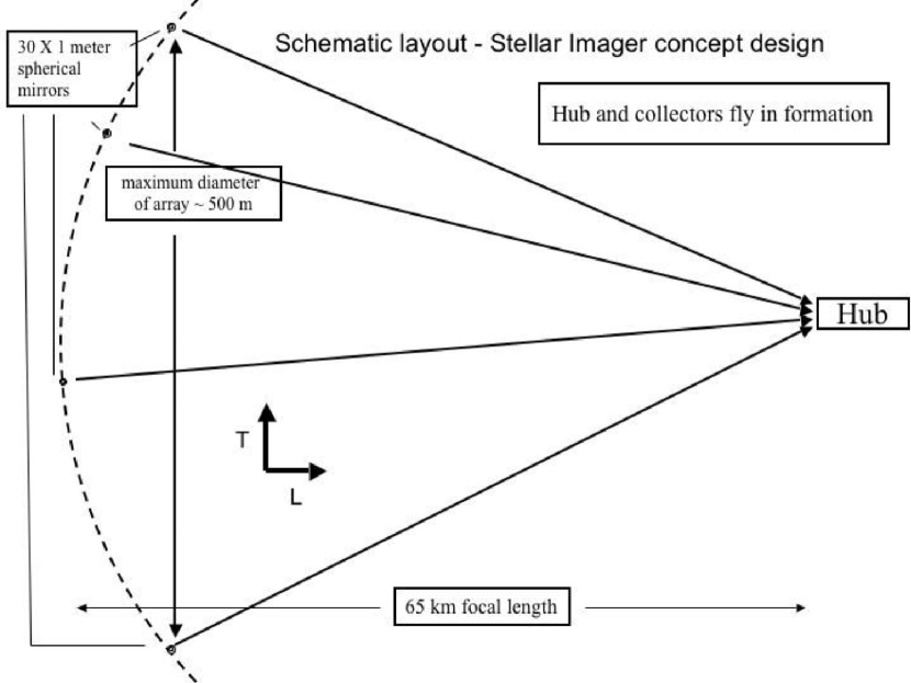
Figure 1: Side view sketch of a possible design for the “Stellar Imager” concept (not to scale). The collectors, which are identical 1-meter spherical mirrors in this design, reflect the light from the target (off to the far right in the figure in the direction indicated by the arrow “L”) to a central hub spacecraft.

Since we can expect that current laser-ranging technology will continue to improve, one can ask whether it might be possible to relax the $\approx\lambda/50$ requirement enough to accomplish station-keeping purely by on-board laser-ranging methods. This would permit the observation of arbitrarily-faint targets located anywhere in the sky. Questions which arise include: How firm is the “$\lambda/50$” requirement? Does the physics of producing images from interferometer fringes justify this number? Are there ways of extracting the desired image information, perhaps only approximately, but which can tolerate larger errors? The search for answers to these questions has motivated the work described in this paper.

An example of the kind of space-based imaging system considered here is shown in Figure 1. This is a cross-section sketch of a concept design for the Stellar Imager, a constellation of about 30 free-flying collectors operating at optical/UV wavelengths and distributed over an area with maximum dimension of up to 500 meters. These collectors direct the radiation they receive to a central “hub” spacecraft for further processing and downlink. Figure 2 shows a possible distribution of the collectors as seen from the central hub.

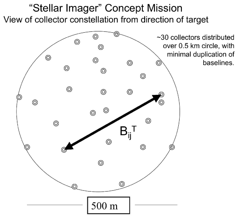
Figure 2: View of the “Stellar Imager” collector constellation from the target showing one of the many interferometer baselines which make up this telescope “aperture”. This view is in the transverse plane (indicated by the arrow “T” in Figure 1), and B${}_{ij}^{T}$ is the distance between any two collectors projected on this plane.

The plan of this paper is as follows. First, a simple (but entirely general) model of the imaging process for free-flying constellations of collectors is described. The basic imaging element of these constellations is the two-element interferometer, and the image quality is particularly sensitive to errors in the determination (and stability) of the phase of the interferometer fringe pattern. This model leads to the identification of two important parameters which play a role in determining the accuracy with which the imaging can be done. The first of these is the projected baseline length, which is the distance between the two collector elements of each constituent interferometer projected on a plane perpendicular to the line of sight to the target, and the second is the optical path difference, which is the difference in the distances from that perpendicular plane through each collector to the interferometer beam combiner.

At this point it is useful to clarify the usage here of the terms knowledge of a parameter and its control. In general, precise control of baseline length is not required; what is required is precise knowledge of the actual values at any time. That knowledge permits us to place a data sample at the right location in the aperture plane before carrying out the imaging computations. On the other hand, precise knowledge of the optical path difference is not sufficient; we must control this quantity to be close to zero at all times. Just how this knowledge and control will be provided will depend on the design of the particular constellation; those details actually do not concern us here, but they will affect the distribution of the error budget over the various parts of the instrument. What does concern us here is to determine the required accuracy on knowledge of the projected baseline length and control of optical path difference in order to achieve a given level of accuracy in the measurements which will go into the final synthesized image. As we shall see, the physics of the interferometric imaging process implies that the typical knowledge accuracy required for the projected baseline length $B_{ij}^{T}$ turns out to depend on the angular size of the target of interest; it is generally at a level of half a meter for typical stellar targets, decreasing to a few centimeters only for the widest practical fields of view. On the other hand, the control accuracy required for the optical path difference OPD is much higher, and depends on the bandwidth of the signal. It is at a level of half a wavelength for narrow (few %) signal bands, decreasing to $\approx 0.2\lambda$ only for the broadest bandwidths expected to be useful. This is a factor 10 less stringent than the rough value of $\lambda/50$ used in the initial exploratory studies mentioned earlier, but exploiting this relaxed value will require post-processing of the interferometer data in a computer.

The paper continues with a brief discussion on translating the two parameters identified into more familiar terms such as the range and bearing from one spacecraft to another. This discussion is sketchy and given only by way of illustration, since the details of specific constellations are not the main topic here. Finally, some implications of these results for the future design of free-flyer imaging systems are discussed. Conventional “direct” imaging systems, which form images directly on a panoramic detector (e.g. a CCD) at the focus of a (“dilute”) aperture, do not easily permit the use of the relaxed requirements on station-keeping described here. “Indirect” imaging systems, where the images are formed by post-processing of interferometer data in a computer, provide opportunities to make use of this (and other ancillary) information, and it is likely that future high-resolution space-based imaging systems for astronomy will be of the indirect type.

Background material on the topics of this paper can be found in several excellent tutorials on the application of interferometry techniques to optical astronomy. For example, see the volume edited by Lawson (2000). Among others, reviews of progress and recent advances have been published by Shao & Colavita (1992) and by Quirrenbach (2001).

2 The Imaging Process

How do we make images using data collected from astronomical targets with a constellation of free-flying collectors? The relevant physics is described mathematically in terms of the mutual coherence function of the wavefront, a quantity which can be measured with an interferometer, and the Van Cittert-Zernike theorem, which relates this mutual coherence function to the object on the sky (i.e. the target brightness distribution) by a Fourier transform. There are numerous textbooks on this topic, see e.g. Born & Wolf (1975); Hecht (2002). The result relevant for now is that, whether the imaging system is “direct”, where an image is instantaneously formed on a 2-dimensional detector (e.g. a dilute-aperture imager), or “indirect”, where an image is formed by post-processing in a computer (e.g. an array of Michelson interferometers), the image is built up by summing fringe patterns formed by the interference of light gathered from all pairs (i,j) of collector elements in the constellation. One such pair, connected as a Michelson interferometer, is sketched in Figure 3.

Figure 3: The basic geometry of an interferometer. Two collectors $i$ and $j$ sample the wavefront from a very distant target at two points separated by $B_{ij}^{T}=B_{ij}\cos\theta$ meters. The two samples are correlated in the beam combiner after experiencing relative path delays of $B_{ij}\sin\theta+d_{i}$ and $d_{j}$, respectively. The beam combiner calculates the fringe parameters, e.g. by scanning $\delta=d_{j}-d_{i}$ over one or two fringe periods, sampling, and fitting the pattern.

At any given wavelength $\lambda$, the interferometer fringe pattern has the form (e.g. Born & Wolf (1975), Chapter 7):

$$P_{ij}=P_{0}[1+A\cos(2\pi k\Delta)],$$ (1)

where $P_{0}$ is the total signal (photons, Joules, etc.) collected by the two elements, $k=1/\lambda$, $A$ is the fringe amplitude, ($0\leq A\leq 1$), and $\Delta$ is the optical path difference (often designated as OPD) composed of:

$$\Delta=B_{ij}\sin\theta+d_{i}-d_{j}.$$ (2)

$\Delta$ is the difference in total path (meters) from the wavefront plane through the two “arms” to the beam combiner, consisting of $B_{ij}\sin\theta+d_{i}$ on the left side of Figure 3, and $d_{j}$ on the right. The angle $\theta$ (in radians, often assumed small so that $\sin\theta\approx\theta$) is measured in the plane containing the interferometer baseline. As we shall see momentarily when we consider detection systems with finite bandwidth, it is important to keep $\Delta\approx 0$, so if $\theta\approx 0$ we shall need to have $d_{i}\approx d_{j}$. This can be achieved by bouncing the light around, in space or in a delay line, before it enters the beam combiner. For instance, if the constellation is deployed on a parabolic surface and the beam combiner is located at the focus of this parabola, then the delays for each collector are “automatically” adjusted to be (nearly) equal. This particular geometry is called a “dilute aperture” since it resembles a conventional reflecting optical telescope with most of the collecting area removed. But this particular geometry is a special case and is not a requirement; the only requirement is that the optical paths somehow be kept nearly equal. We also define the fringe period measured on the sky as $\lambda/B_{ij}^{T}$ radians. Note that the fringe period increases as the projected baseline decreases with increasing $\theta$. Note also that a typical system at optical wavelengths may have $B_{ij}^{T}/\lambda\approx 1\times 10^{9}$ and $\theta\approx 3-100\times 10^{-10}$ rads, or $\approx 60-2000\>\mu$as.

It is convenient to simplify the way we write the fringe pattern by defining the quantities $\phi_{T}=kB_{ij}\sin\theta$ and $\phi_{I}=k(d_{j}-d_{i})$, both in units of “turns”, so that Equation 1 becomes:

$$P_{ij}=P_{0}\{1+A\cos[2\pi(\phi_{T}-\phi_{I})]\},$$ (3)

where $\phi_{T}$ is called the fringe phase and depends on the location of the target on the sky, and $\phi_{I}$ is the instrument phase, which can be controlled by altering the internal delay difference $d_{j}-d_{i}$. The elemental narrow-band fringe pattern of Equation 3 is sketched as a function of instrument phase in the top panel of Figure 4. Note that the structure of the fringes can be determined by scanning the instrument phase $\phi_{I}$ over one or two turns and fitting the resultant fringe pattern to Equation 3, thereby obtaining the total power, the fringe amplitude, and the fringe phase. This form of the equation also makes it clear that errors in the instrument phase $\phi_{I}$, such as those arising from station-keeping errors, directly masquerade as changes to the measured value of fringe phase $\phi_{T}$, and therefore to errors in the measured position $\theta$ of the target. Finally, Figure 4 also makes it clear that the position of the target in the field of view is obtained by counting fringes (and fractions thereof) from a reference point, for example the direction where $\phi_{I}=0$.

Figure 4: Top panel: Fringe pattern $P_{ij}$ from Equation 3 for baseline $B$ as a function of fringe phase $\phi_{T}$ in “turns” (see text). The instrument phase is assumed to be at $\phi_{I}=0$. Bottom panel: Fringe pattern for a baseline which is in reality 5% larger. Notice that the error grows with angular distance from the point where $\phi_{I}=0$, reaching $\approx 0.15$ fringes ($54^{\circ}\approx 1$ rad) at the edge of this small 3-fringe field. The y-axis is in units of the signal strength obtained by a single collector.

The discussion so far has assumed that the interferometer is sensitive to only one wavelength, i.e. that the bandwidth of the detection system is infinitely narrow. The fringe pattern for a finite bandwidth detection system is the weighted (vector) sum of the fringe patterns at all constituent wavelengths, with amplitudes specified by the product of the source spectrum and the instrument response at each wavelength. A simple but illustrative case which is easy to calculate is for a rectangular bandpass of central wavelength $\lambda_{0}$ and width $\delta\lambda$, and a target spectrum that is flat over this wavelength range. In this case the resulting fringe pattern is:

$$P_{ij}=P_{0}[1+\frac{\sin(\pi\Delta/L_{c})}{\pi\Delta/L_{c}}\times A\cos(2\pi k_{0}\Delta)],$$ (4)

where the symbols not already defined in the previous two equations are $k_{0}=1/\lambda_{0}$, and $L_{c}=\lambda_{0}^{2}/\delta\lambda$. This latter quantity is called the coherence length for the light beam, a concept which arises as follows (Born & Wolf (1975), Ch. VII; Hecht (2002), Ch. 7): For a finite detector bandwidth of $\delta\nu$ hertz, the signal in free space is a compact packet of many interfering waves with a coherence time of $\tau=1/\delta\nu$ seconds. Expressing the bandwidth in terms of wavelength, we have $\delta\nu=-(c/\lambda_{0}^{2})\times\delta\lambda$, so the coherence time $\tau=(-1/c)\times(\lambda_{0}^{2}/\delta\lambda)$, and $c\,\tau$ is a scale size of the wave packet called the coherence length, $L_{c}=c\,\tau=\lambda_{0}^{2}/\delta\lambda$. The lower panel of Figure 6 shows a sketch of this situation for $\delta\lambda/\lambda_{0}=0.2$. Note that, within a few fringes of the central peak, the finite-bandwidth fringe in the lower panel shows the same periodicity (and positioning, or fringe phase) as the single-wavelength case in the upper panel. This means that the relative placement of different components of the reconstructed target brightness distribution will be correct, but their amplitudes may be wrong. Perhaps even more serious, the signal-to-noise ratio of the amplitude measurement will be worse.

We are now in a position to begin the discussion on the accuracy with which the relative positions of the collectors need to be known. For completeness, note that we are here focussing only on that part of the error budget which arises because of errors in the station-keeping. A full discussion of all error sources and their various contributions is, of course, dependent on the design details of each specific constellation.

3 Two Requirements

Inspection of Equations 1, 2, and 4 above makes it clear that, in order to apply these equations to real data, there are two parameters which depend on station-keeping and which are important for each interferometer in the constellation: the length of the projected baseline $B_{ij}^{T}$, and the optical path difference $\Delta$ at the beam combiner. The accuracy requirements on these two parameters are presented below first by stating the result, then providing the derivation, and finally discussing some of the implications.

3.1 Baseline

The fractional accuracy $\delta B_{ij}^{T}/B_{ij}^{T}$ with which the projected distance between any i,j collector pair in the transverse plane must be known is:

$$\delta B/B\lesssim 1/(N_{f}\,Q_{T}).$$ (5)

where $N_{f}$ is the number of fringes in the angle $\rho$, $\rho$ is the angular radius of the field of view containing the object being imaged, and $Q_{T}$ is the “transverse quality factor” expressing the accuracy $\lambda/Q_{T}$ with which the “optical figure” of the imaging system is to be held. The super- and subscripts of $B$ have been dropped for convenience.

3.1.1 Demonstration:

The fringe pattern for an elemental interferometer expands and contracts about the field center as B decreases or increases owing to station-keeping errors, and for a given (but in reality unknown) baseline error of $\delta B$ the resulting fringe phase error grows with angular distance from the center of the field. The situation for the narrow-band case is sketched in Figure 4.

Without loss of generality we can take the center of the fringe pattern to be the centroid of the target brightness distribution at the operating wavelength $\lambda$. Let $\rho$ be the angular radius (in radians) of a circle on the sky which is just large enough to include all the emission from the target. The number $N_{f}$ of fringes in $\rho$ is $N_{f}=\rho/(\lambda/B)$. This number changes with small changes in the baseline length according to $\delta N_{f}=\rho\,\delta B/\lambda$. Substituting for $\rho$ from the initial expression for $N_{f}$ results in $\delta N_{f}=N_{f}\times\delta B/B$. If we require that the optical quality of the signal provided by this interferometer be better than a fraction $1/Q_{T}$ of a wavelength, then we must have $\delta N_{f}\lesssim 1/Q_{T}$. From this we derive $\delta B/B\lesssim 1/(N_{f}\,Q_{T})$, which proves the result.

3.1.2 Discussion:

As an example, suppose the source is a distant star and the instrument is intended to provide 30 independent resolution elements across the stellar diameter. Each resolution element is of angular size $\lambda/B_{max}$ radians, where $B_{max}$ is the longest (projected) baseline in the constellation. Suppose further that it can be safely assumed there is no signal outside a larger circle of some given angular radius, say $\rho=20\times\lambda/B_{max}$ radians on the sky measured from the center of the star. For this example, $N_{f}\approx 20$. If we demand an “optical quality” of, say, $\lambda/50$ in our imaging instrument, then $Q_{T}=50$ and $\delta B/B\lesssim 1/1000$. For a maximum baseline of $B=500$ meters, the largest unknown $\delta B$ we can tolerate is $\approx 0.5$ m. Note that since $N_{f}\propto B$ for a given source size and operating wavelength, $\delta B$ is actually independent of $B$, so the required accuracy in this example is the same for every baseline in the constellation. However, the stringency of the requirement grows with the size of the target field of view in the sky. For instance, for a supergiant star the desired FOV could be a factor of 10 larger than the example calculated above, and the required tolerance on any baseline would be $\approx 5$ cm. But now such a constellation would provide 300 independent resolution elements across the star. If the science goals permit, it may be more prudent to “shrink” the overall extent of the constellation by a factor 10 in order to return to the scale of the initial example and relax the station-keeping requirements accordingly.

It is interesting to ask what the limit on $\delta B/B$ might be for very large fields of view. For instance, for a Michelson radio interferometer with a single “feed horn” at the focus of each collector, the largest field of view will be limited by the diffraction pattern of the individual collector elements. This field has an angular radius $\approx\lambda/a$ where $a$ is the diameter of a collector element. In this extreme case, $N_{f}\approx B/a$, so the maximum tolerable error is:

$$\delta B/B\lesssim 1/(N_{f}\,Q_{T})\approx a/(B\,Q_{T});$$ (6)

i.e., $\delta B\lesssim a/Q_{T}$, which depends only on the size of the elements in the constellation. If a typical collector is one meter in diameter and $Q_{T}=50$, the required knowledge accuracy is $\approx 2$ cm. The situation gets more demanding if a wide field beam combiner is used, such as an optical Michelson interferometer with detector pixels that are larger than the collector diffraction pattern, or with many independent pixels in the detection system.

To conclude this section, note that changes in operating wavelength have similar effects on the array reponse to those discussed above and can be modelled in the same way. One particularly deleterious effect of this is that the point spread function of a system with a finite spectral resolution will vary over the field of view, becoming radially elongated at large angular distances. Such effects were first analysed in detail by radio astronomers modeling the reponse of ground-based radio synthesis imaging arrays (see e.g. Thompson (1994)).

3.2 Optical Path Difference

The accuracy $\delta\Delta$ with which the optical path difference must be controlled to zero is:

$$\delta\Delta/\lambda_{0}\lesssim(1/Q_{OPD})\times(\lambda_{0}/\delta\lambda).$$ (7)

where $\delta\lambda/\lambda_{0}$ is the fractional bandwidth of the signal and $Q_{OPD}$ is the “OPD quality factor”, by analogy to the $Q_{T}$ factor defined earlier. This requirement can also be written as $\delta\Delta\lesssim L_{c}/Q_{OPD}$, where $L_{c}$ is the coherence length defined following Equation 4.

3.2.1 Demonstration:

Some clarification is needed first, since the real problem here may not be entirely obvious. It is clear from Equation 1 that errors of $\delta\Delta/\lambda$ directly translate to a fringe error of $G\,\delta\Delta/\lambda$ where $G$ is a geometry-dependent factor of order unity depending on the specific geometry of the constellation. However, in this case it is not an expansion or contraction of the fringe pattern about the field center, but a gross translation of the entire fringe pattern in a direction parallel to that of the baseline projection on the field of view. At first sight this is a serious problem, since it appears to require holding the collector positions to a tiny fraction of the wavelength. However, since it is the whole fringe pattern that moved and not the relative separation between two points in the field of view, the angular distance measured in fringes between the center and the edge of the field remains the same. In other words, the relative fringe phase is actually not sensitive to this shift! Figure 5 shows a sketch of the situation.

Figure 5: Top panel: Narrow-band fringe pattern from Figure 4. Bottom panel: Narrow-band fringe pattern shifted by a phase error of $\delta\phi=1$ rad, caused e.g. by an OPD error of $\delta\Delta\approx\lambda/6$.

If we can design our system and/or (post-) process the data in order to use this “relative” phase insead of an “absolute” phase, we would be entirely insensitive to OPD errors, although we would lose the ability to measure the target position in an absolute sense. Except for accurate wide-angle astrometry, no other applications in astrophysics require such absolute position information. The real problem comes about because of a loss of fringe amplitude at large non-zero values of the OPD owing to the finite bandwidth of the detection system. Only if the bandwidth is infinitely narrow will the fringe pattern amplitude remain independent of the OPD error $\delta\Delta$ as shown e.g. in the upper panel of Figure 6; the lower panel of this figure shows a “real” fringe pattern for a finite (20%) bandwidth following Equation 4. It is clear that, as the OPD error grows, so does the error in the measurement of the fringe amplitude. The scale size of the fringe pattern envelope is characterized by the coherence length $L_{c}$ as shown in Equation 4. If we can keep the OPD error $\delta\Delta$ to some fraction $1/Q_{OPD}$ of the coherence length $L_{c}$, then this amplitude error can be minimized and the measurement of fringe amplitude and fringe phase can be made subject only to photon noise in the time scale of the drift in the station position. This requirement becomes $\delta\Delta\lesssim(1/Q_{OPD})\times L_{c}$ or $\delta\Delta/\lambda_{0}\lesssim(1/Q_{OPD})\times(\lambda_{0}/\delta\lambda)$, which proves the result.

Figure 6: Top panel: Fringe pattern as a function of OPD error (in wavelengths) for a very narrow-band signal. Bottom panel: The same fringe pattern for a square bandpass of 20%. Note how the fringes disappear beyond $N_{f}\approx 5$.

3.2.2 Discussion:

As an example, for $Q_{OPD}=50$ and a bandwidth of a few %, say $\lambda_{0}/\delta\lambda\approx 30$, the control requirement on $\delta\Delta$ is $0.6\,\lambda$. This requirement will still be difficult to achieve at optical wavelengths, but now there is a better chance that on-board laser ranging systems may eventually provide adequate position knowledge without the use of signal photons, thereby allowing long integrations on faint sources. Bandwidths in excess of $\approx 10\%$ in a single detector channel are not likely to be used since the spectral dependence of the fringe pattern is often an important diagnostic for the on-board fringe detection algorithms. This means that the worst case for the control accuracy of the OPD (which is essentially the station-keeping requirement, as we shall see below) is $\approx 0.2\,\lambda_{0}$, still a factor of 10 less stringent than the early estimates of $0.02\,\lambda_{0}$ mentioned in the introduction to this paper.

Now that the two major physical quantities have been identified, and their accuracy requirements estimated, we can consider how to apply these criteria to real cases of specific mission concepts.

4 Applications to Specific Mission Concepts

The previous section has identified the two physical parameters $B$ and $\Delta$ which characterize the constituent fringe patterns that go into building an image from data obtained with a constellation of free-flying collectors. In order to take the next step of translating the general knowledge requirements on $\delta B$ and $\delta\Delta$ into nanometers and microradians for a specific mission concept, we need to distinguish two cases depending on the brightness of the targets to be observed.

4.1 Bright Targets

If enough photons will be available to operate a servo loop to keep the optical path difference $\Delta\approx 0$ to within some fraction of the coherence length $L_{c}$, then the control requirement on $\delta\Delta$ need not translate into a station-keeping requirement, but rather into a requirement on the total stroke and accuracy of the on-board delay line. In this case we are left only with the knowledge requirement on the projected baseline length which depends on the size of the target field of view, as stated in Equation 5. The requirement on the accuracy in the range from one spacecraft to another is of order half a meter. This still permits imaging of the stellar surface with a relative resolution of about 30. An error in the bearing of the second spacecraft with respect to the first in the interferometer pair also appears as an error in the projected baseline, but this component will be less significant; from the geometry of the interferometer in Figure 3 it is easy to show that an error of $\delta\alpha$ in the bearing translates into a fractional projected baseline error of $\delta B/B\approx(\delta\alpha)^{2}/2$. For the example taken in §3.1, $\delta B/B\lesssim 1/1000$, so the requirement on the bearing is 0.1 rad $\approx 1^{\circ}$ independent of B.

4.2 Faint Targets

If we want to observe faint (or partially resolved) targets which do not provide enough photons to properly operate a control loop on the optical path difference, then Equation 7 drives the station-keeping requirement. Errors in station-keeping map into errors in $\Delta$ in a manner dependent on the specific constellation geometry. For instance, for a design where the beam combiner lies between the two collectors (as in the TPF-I concept), a station-keeping error of $\delta B$ in the baseline length will produce a delay error of $\delta\Delta=\delta B$, and we have seen from the demonstration following Equation 7 that such errors need to be kept smaller than some fraction $1/Q_{OPD}$ of the coherence length. If laser ranging is available and capable of measuring the baseline length to sufficient precision, then that information could be fed to an on-board delay line in the target signal path to correct for baseline length errors. This would turn the requirement on $\delta B$ from a control requirement into a knowledge requirement.

Bearing errors $\delta\alpha$ also directly translate into delay errors; for the SI concept of Figure 1 this is $\delta\Delta\approx B\delta\alpha$, so the knowledge of bearing of the second spacecraft with respect to the first is $\delta\alpha\lesssim L_{c}/(BQ_{OPD})$ which for sample values used in the discussion in §3.2 becomes $\delta\alpha\lesssim 0.6\,\lambda/B$ rads or $\approx 0.1$ milli-arcseconds for $B=500$ m and $\lambda=500$ nm. This will be a difficult requirement to meet if the collectors in the constellation are all more-or-less in a plane. Placing an additional “metrology” spacecraft some distance from this plane (e.g. in the “Hub” spacecraft for the SI design of Figure 1) would alleviate the requirement by converting the inter-collector bearing measurement for station-keeping errors in the direction to the target (the “L” direction in Figure 1) to a range measurement (with the usual required accuracy of order $L_{c}/Q_{OPD}$) from a collector to the metrology spacecraft.

5 Indirect Imaging

In order to take advantage of the relaxed control requirement on the optical path difference described in Equation 7, we must find a method of turning the recorded fringe amplitudes and (slowly-drifting) phases into an image in such a way as to be insensitive to shifts of the whole fringe pattern owing to small OPD errors. There are several related “post-processing” techniques which could be used for this. For instance, if the field of view contains a bright star besides the target of interest, fringe phases could be “referenced” to this star. Another approach (first used at radio wavelengths) is to reference phases to a bright spectral line feature.

One quite general approach to this “unstable-phase” imaging problem which has been used with success for $\approx 40$ years in the radio astronomy community uses the concept of “closure phase”. Almost 50 years ago, Jennison (1958) presented a technique for measuring relative fringe phase which used three radio-linked collectors coupled as three interferometers operating at a wavelength of 2.4 meters over baselines up to $\approx 10$ km. Owing to a variety of instrumental problems related to the amplifiers and local oscillator electronics available at the time, the fringe phase between any two collectors was unstable and could normally not be measured; the source structure information had to be derived from the (squared) fringe amplitudes alone (a familiar situation in present-day ground-based optical interferometry). Jennison showed that, if the three observed fringe phases were summed, the resultant combined phase was insensitive to equipment instabilities. With this approach, Jennison & Latham (1959) showed that the brightness distribution of the radio source Cygnus A, which until then was only known to be elongated, actually consisted of two separated sources of nearly equal brightness straddling a peculiar optical object tentatively identified at the time with two galaxies in collision. This was the first observation to reveal the double-lobed structure of a powerful radio galaxy.

Applications of this method to circumvent atmospheric phase instabilities in optical interferometry were described by Jennison (1961) and, apparently independently, by Rogstad (1968). The first use of the term “closure phase” seems to be in the paper by Rogers et.al. (1974) describing an application at radio wavelengths using very stable and accurate, but independent, reference oscillators at the three stations in a so-called “very-long-baseline” interferometer array. Since that time, closure phase has been used extensively at radio, IR, and optical wavelengths, and there are many papers describing the subject, its virtues, and its limitations. Monnier (2003) gives a review of optical interferometry in astronomy which includes a discussion of closure phase, and also points out the intimate relationship between it and the complex bispectrum, a quantity constructed in processing optical speckle interferometry data. For the type of collector constellations discussed in this paper, the phase of the complex bispectrum is precisely the closure phase, and by (vector) averaging the complex bispectrum the closure phases can be obtained in principle for arbitrarily faint targets. One important point to make here is that use of such techniques requires that the fringe signals from each pair of collectors be separable one from another, such that the individual interferometer fringe phases can be uniquely assigned to the appropriate pair of collectors. This leads in turn to requirements on the design of the optics at the location where the collector beams are brought together to interfere.

6 Conclusions

The requirements on station-keeping for constellations of free-flying collectors coupled as (future) imaging arrays in space for astrophysics applications have been discussed. The typical knowledge accuracy required on the projected baseline of the instrument depends on the angular size of the targets of interest; it is generally at a level of half a meter for typical stellar targets, becoming of order a few centimeters only for the widest attainable fields of view. The typical control accuracy required on the optical path difference depends on the wavelength and the bandwidth of the signal, and is at a level of half a wavelength for narrow (few %) signal bands, becoming $\approx 0.2\,\lambda$ for the broadest bandwidths expected to be useful. If the fringe detection system is able to use signal photons or photons from a nearby reference star, then the most stringent requirement on station-keeping is that on the baselines, as described in §3.1. If observations on faint targets are required, and fringe tracking is “blind”, then the most stringent requirement on station-keeping is that on the optical path difference described in §3.2. If on-board laser metrology is available and can provide knowledge of the internal OPD to a fraction of the target signal coherence length, then active fringe tracking could compensate for station-keeping errors, even for faint sources.

In any case, the requirements are less severe than assumed in the early studies of the problem. The significance of this result is that, at this relaxed level of accuracy, it may be possible to provide the necessary knowledge of array geometry without the use of signal photons, thereby allowing observations of arbitrarily-faint targets.

Such constellations of free-flyers will produce images using various computer-based image reconstruction techniques which relax the level of accuracy required on the fringe phase stability of each component interferometer. “Closure-phase” imaging is one such technique which has been very successfully applied in ground-based radio and optical astronomy in order to surmount instabilities owing to equipment and to the atmosphere. This technique appears to be directly applicable to space imaging arrays, where station-keeping drifts play the same role as atmospheric and equipment instabilities. More detailed modeling of anticipated station-keeping errors and their effects on synthetic images is needed. For instance, there is at present little justification for the values “$Q_{OPD}=Q_{T}\approx 50$” used repeatedly in this paper. A study needs to be done of the degradation in image quality as these parameters are diminished (and the OPD and baseline errors grow), as well as a comparison of the merits of various image reconstruction algorithms including the use of closure phase and bispectrum analysis.

References

- Born & Wolf (1975) Born, M., & Wolf, E. 1975, Principles of Optics (Fifth Edition) (Pergamon Press)
- Cornwell (1987) Cornwell, T.J. 1987, A&A, 180, 269
- ESA (1996) ESA Report SCI(96)7 1996, Kilometric Baseline Space Interferometry, (European Space Agency, Paris)
- Hecht (2002) Hecht, E. 2002, Optics (4th edition) (Addison Wesley)
- Jennison (1958) Jennison, R.C. 1958, MNRAS, 118, 284
- Jennison & Latham (1959) Jennison, R.C., & Latham, V. 1959, MNRAS, 119, 174
- Jennison (1961) Jennison, R.C. 1961, Proc. Phys. Soc. 78, 596
- Jones (1991) Jones, D. 1991, in Technologies for Optical Interferometry in Space, ed. S. P. Synnott (JPL Pub. D-8541), 177-181.
- Lawson (2000) Lawson, P.R. 2000, Principles of Long Baseline Stellar Interferometry (JPL Pub. 00-009161616Also at http://olbin.jpl.nasa.gov/papers/index.html)
- Monnier (2003) Monnier, J.D. 2003, Reports on Progress in Physics, 66, 789
- Quirrenbach (2000) Quirrenbach, A. 2000, “Phase Referencing,” in Principles of Long Baseline Stellar Interferometry, ed. P. R. Lawson (JPL Pub. 00-009), 143
- Quirrenbach (2001) Quirrenbach, A. 2001, ARA&A, 39, 353
- Rogstad (1968) Rogstad, D.H. 1968, Applied Optics, 7, 585
- Rogers et.al. (1974) Rogers, A.E.E, et al. 1974, ApJ, 193, 293
- Shao & Colavita (1992) Shao, M., & Colavita, M.M. 1992, ARA&A, 30, 457
- Thompson (1994) Thompson, A.R. 1994, “The Interferometer in Practice,” in Synthesis Imaging in Radio Astronomy, eds R.A. Perley, F.R. Schwab, & A.H. Bridle, ASP Conference Series, Vol. 6 (Astron. Soc. of the Pacific, San Francisco), 11