A Statistical Theory for Measurement and Estimation
of Rayleigh Fading Channels

Abstract

In this paper, we propose a statistical theory on measurement and estimation of Rayleigh fading channels in wireless communications and provide complete solutions to the fundamental problems: What is the optimum estimator for the statistical parameters associated with the Rayleigh fading channel, and how many measurements are sufficient to estimate these parameters with the prescribed margin of error and confidence level? Our proposed statistical theory suggests that two testing signals of different strength be used. The maximum likelihood (ML) estimator is obtained for estimation of the statistical parameters of the Rayleigh fading channel that is both sufficient and complete statistic. Moreover, the ML estimator is the minimum variance (MV) estimator that in fact achieves the Cramér-Rao lower bound.

1 Introduction

In mobile radio channels, the Rayleigh distribution is commonly used to describe the statistical nature of the received envelope of a flat fading signal, or the envelope of an individual multipath component. Flat fading is often associated with the narrow band channel. By assuming that the real and imaginary parts of the channel gain are independent Gaussian random variables with zero mean and equal variance, the amplitude of the channel gain or PL (path loss) becomes a Rayleigh random variable. For wide band channels, multipath gains are typically assumed to be uncorrelated scattering (US) and each path gain is wide-sense stationary (WSS) which are termed as WSSUS channels [2]. By assuming that the real and imaginary parts of each path gain are independently Gaussian distributed with zero mean and equal variance, the amplitudes of the multipath gains become independent Rayleigh random variables. Theoretically a Rayleigh random variable is uniquely specified by its 2nd moment that is the sum of the variances of its two independent Gaussian components. In practice the statistics of the Rayleigh fading channel are incomplete without additional knowledge of the noise power and SNR (signal-to-noise ratio). That is, the statistical parameters of the channel power, noise power, and SNR together characterize the Rayleigh fading channel completely, giving rise to the measurement and estimation problem for these statistical parameters.

Estimation for the 2nd moment of a Rayleigh random variable has practical importance in channel modeling and estimation [3, 9, 12], and in radio coverage, location, and measurement [4, 8]. For these reasons statistical estimation of Rayleigh fading channels has been studied and reported in the existing research literature. The early work of Peritsky [13] shows that the simple averaged square of the signal strength based on i.i.d. (independent and identically distributed) measurement samples is both an ML (maximum likelihood) and MV (minimum variance) estimator, and such an averaged square is a sufficient and complete statistic. However his results focus only on the noise-free case and have limited applications. The same problem has been investigated in [1, 6, 7, 10, 11, 19, 20] that encompass the Ricean and Nakagami fading distributions, as well as MIMO fading channels. But there lack optimum estimators that achieve the Cramér-Rao lower bound.

In this paper we propose a statistical theory on measurement and estimation of Rayleigh fading channels. Our contributions include derivation of explicit a priori bounds on the measurement sample size that achieve the prescribed margin of error and the confidence level, and discovery of the optimum estimator that is both an ML and MV estimator, and achieves the Cramér-Rao lower bound. These results complement the existing work reported in the literature, In the noise-free case our sample size bound resembles the one implicitly indicated in [5] which asserts that, to estimate the binomial probability with the prescribed margin of absolute error $\varepsilon$ and confidence level $1-\delta$, it suffices to have a sample size greater than $\frac{\ln(\frac{2}{\delta})}{2\varepsilon^{2}}$. One notable difference is that our sample size bound is derived for the relative error while the bound in [5] is derived for the absolute error in estimation of the binomial probability. Furthermore an interval estimate similar to that in [13] is obtained with much simpler calculation.

In applications to Rayleigh fading channels, noisy measurement samples have to be taken into consideration. Our proposed statistical theory suggests that two testing signals of different strength be used. The use of two different testing signals enables us to extend the sample complexity results from the noiseless case to the noisy case which solves the sample complexity problem not only for the 2nd moment or the mean channel power, but also for the mean noise power and for the SNR. The explicit a priori bounds resemble to those in the noise-free case of which the sample size is roughly inversely proportional to the square of the margin of error and is linear with respect to the logarithm of the inverse of the gap between the confidence level and $1$. Our results show that a typical margin of error can be achieved with near certainty and modest sample size. More importantly an optimum estimator is obtained for noisy Rayleigh fading channels that is both an ML and MV estimator. It inherits the same sufficient and complete statistic property from that in the noiseless case [13], and it achieves the Cramér-Rao lower bound.

The content of the paper is organized as follows. In Section 2 we first present the Rayleigh fading channel and its associated measurement and estimation problem in terms of the sample complexity and the optimum estimator. The sample complexity problem is then addressed in Section 3 by establishing an explicit a priori bound on the sample size that is asymptotically tight based on noiseless measurements. In Section 4 we present our main results on parameter estimation for Rayleigh fading channels by taking the noisy measurement samples into consideration to which complete solutions are derived for measurement and estimation of Rayleigh fading channels. Numerical examples are presented in Section 5 to illustrate our results, and the paper is concluded in Section 6. The notations are standard and will be made clear as we proceed.

2 Rayleigh Fading Channels

In a typical urban environment, there is no LOS (line of sight) between the transmitter and the receiver. The wireless channel is characterized by multipath and follows the Rayleigh distribution. Specifically a widely used channel model is the following continuous-time CIR (channel impulse response):

$$c(t;\tau)=\sum_{n=0}^{N}\alpha_{n}(t)e^{j\beta_{n}(t)}\delta\left(t-\tau_{n}(t)\right)$$ (1)

where $\alpha_{n}(t)$, $\beta_{n}(t)$, and $\tau_{n}(t)$ are the amplitude, phase, and time delay, respectively, associated with the $n$th path, and $\delta(\cdot)$ is the Dirac delta function. For narrow band systems, the channel gain is given by

$$H(t)=H_{R}(t)+jH_{I}(t):=\left[\sum_{n=1}^{N}\alpha_{n}(t)\cos(\phi_{n}(t))\right]+j\left[\sum_{n=1}^{N}\alpha_{n}(t)\sin(\phi_{n}(t))\right]$$ (2)

The arguments $\{\phi_{n}(t)\}$ are due to $\{\beta_{n}(t)\}$ and $\{\tau_{n}(t)\}$ induced by Doppler shifts and time delays that form a set of independent random variables uniformly distributed over $[-\pi,\;\pi]$. Under the assumption that $\alpha_{n}(t)\equiv\alpha_{n}$, $\beta_{n}(t)\equiv\beta_{n}$, and $\tau_{n}(t)\equiv\tau_{n}$, $H(t)$ becomes a WSS (wide-sense stationary) process. For large $N$, the central limiting theorem can be invoked to treat both $H_{R}(t)$ and $H_{I}(t)$ as independent Gaussian random processes with zero mean and equal variance [14, 18]. This gives rise to the Rayleigh fading channel in light of the fact that $|H(t)|^{2}$ is a Rayleigh random variable. For wide band systems, multipath gains can be resolved up to the resolution dictated by the sampling frequency $f_{s}$. An equivalent discretized CIR can be represented by

$$H(t)=\sum_{k=0}^{L-1}H_{k}(t)\delta_{t-kT_{s}},\;\;\;\;\;T_{s}=f_{s}^{-1}$$ (3)

in which $|H_{k}(t)|^{2}$ is Rayleigh distributed for $0\leq k<L$ where $\delta_{t}$ is the Kronekar delta function.

Rayleigh fading channels are widely used in wireless communications. An important and practical problem is measurement of $|H(t)|^{2}$ and estimation of $\mathbb{E}[|H(t)|^{2}]$, with $\mathbb{E}[\ \cdot\ ]$ the expectation, for narrow band systems, or $|H_{k}(t)|^{2}$ and power delay profile $\mathbb{E}[|H_{k}(t)|^{2}]$ for wide band systems. Such a problem is crucial in modeling and estimation of wireless channels, and in radio coverage and location. A common strategy is to transmit i.i.d. pilot symbols or testing signals to obtain measurement samples of $|H(t)|^{2}$ or $|H_{k}(t)|^{2}$, and then to estimate the mean. For simplicity we drop the time argument $t$, and focus on narrow band systems but our results are applicable to wide band systems as well by converting frequency-selective fading channels into flat fading channels using the OFDM (orthogonal frequency division multiplexing) scheme [12]. The detail is omitted.

Denote $\Re[C]$ as the real part of the complex number $C$. Let the transmitted symbol be $S$. In the complex form, the received signal can be written as (“$\Longrightarrow$” stands for “implying”)

$$x(t)=\Re[(HS+V)e^{j2\pi f_{c}t}]\;\;\;\;\Longrightarrow\;\;\;\;X=HS+V$$ (4)

where $f_{c}$ is the carrier frequency and $V=V_{R}+jV_{I}$ is the complex additive Gaussian noise with zero mean and equal variance $\sigma_{V}^{2}$. Since the average power of the transmitted signal is $P_{s}=\mathbb{E}[|S|^{2}]$ and the average power of the received signal is $\mathbb{E}[|HS|^{2}]$, the channel power or PL is

$${\rm PL}=10\log_{10}\left(\frac{\mathbb{E}[|S|^{2}]}{\mathbb{E}[|HS|^{2}]}\right)=10\log_{10}\left(\frac{\mathbb{E}[|S|^{2}]}{\mathbb{E}[|H|^{2}]\;\mathbb{E}[|S|^{2}]}\right)=-10\log_{10}\left(\mathbb{E}[|H|^{2}]\right)=-10\log_{10}\left(2\sigma_{H}^{2}\right)$$

where $\sigma_{H}^{2}$ is the common variance of $H_{R}$ and $H_{I}$. It can be seen that $\sigma_{H}^{2}$ depends on the attenuation factors $\{\alpha_{n}\}$ that decrease as the receiver is further away from the transmitter. It follows that $\sigma_{H}^{2}$ and thus SNR become small when the receiver is far away from the transmitter. To predict the coverage and the performance of wireless systems, it is important to know the operating range of the SNR at different locations. The SNR at the receiver is easily found to be

$${\rm SNR}=10\log_{10}\left(\frac{\mathbb{E}[|HS|^{2}]}{\mathbb{E}[|V|^{2}]}\right)=10\log_{10}\left(\frac{\mathbb{E}[|S|^{2}]\;\mathbb{E}[|H|^{2}]}{\mathbb{E}[|V|^{2}]}\right)=10\log_{10}\left(\mathbb{E}[|S|^{2}]\right)+10\log_{10}\left(\frac{\sigma_{H}^{2}}{\sigma_{V}^{2}}\right)$$

where $\sigma_{V}^{2}$ is the common variance of $V_{R}$ and $V_{I}$. Since $P_{s}=\mathbb{E}[|S|^{2}]$, the average power for transmitting the symbol $S$, is computable, to obtain an estimate for the SNR it is necessary to have an estimate for the ratio of $\sigma_{H}^{2}$ to $\sigma_{V}^{2}$. However it remains unclear whether or not the knowledge of SNR helps to estimate the PL that will be investigated later. Our main results to be presented show that with appropriate signaling, the variances $\sigma_{H}^{2}$, $\sigma_{V}^{2}$, and the SNR can all be estimated in satisfaction.

The objective of this paper is in fact beyond estimation of the PL that has been investigated by several researchers [7, 10, 11, 13, 19, 20]. Our goal is to develop a relevant statistical theory in order to derive an optimum estimator for the statistical parameters associated with the Rayleigh fading channel, and to derive a priori sample complexity bounds given the prescribed margin of error and the confidence level. These two problems are not completely solved in the existing research literature that will be studied thoroughly in the next several sections. We will begin with the ideal case of noiseless measurements by assuming independent PSK (phase shift keying) or BPSK (binary PSK) signaling at the transmitter leading to $N$ independent measurement samples $\{X_{i}\}_{i=1}^{N}$ at the receiver. In light of [13],

$$\widehat{\sigma_{H}^{2}}=\frac{\overline{X_{N}^{2}}}{P_{s}},\;\;\;\;\;\overline{X_{N}^{2}}=\frac{1}{2N}\sum_{i=1}^{N}|X_{i}|^{2}$$ (5)

is an ML estimator for $\sigma^{2}_{H}$ that is both statistically sufficient and complete. We thus have an equivalent problem for estimation of the 2nd moment of the Rayleigh random variable based on its $N$ i.i.d. samples. The complete results on sample complexity in this case will be presented in the next section.

After solving the sample complexity problem in the noise-free case, we will investigate the sample complexity problem in estimation of the PL, the noise power, and the SNR, associated with Rayleigh fading channels based on noisy measurement samples. Two sets of independent BPSK signals $\{S_{1,i}\}_{i=1}^{N_{1}}$ and $\{S_{2,i}\}_{i=1}^{N_{2}}$ are transmitted with difference in their average power: $|S_{1,i}|^{2}=P_{s1}$ and $|S_{2,i}|^{2}=P_{s2}$ for all possible $i$ where $P_{s1}>P_{s2}\geq 0$. The following two quantities

$$\overline{X_{1,N_{1}}^{2}}=\frac{1}{2N_{1}}\sum_{i=1}^{N_{1}}|X_{1,i}|^{2},\;\;\;\;\;\overline{X_{2,N_{2}}^{2}}=\frac{1}{2N_{2}}\sum_{i=1}^{N_{2}}|X_{2,i}|^{2}$$ (6)

turn out to be sufficient and complete statistics in statistical estimation of the Rayleigh fading channel based on noisy samples. In fact the optimum estimator is obtained that achieves the Cramér-Rao lower bound. Complete results are obtained and will be presented in a later section.

3 Sample Complexity in the Noiseless Case

As discussed earlier estimation of the 2nd moment for the Rayleigh fading channel in the noise-free case is equivalent to that for the Rayleigh random variable. Let $X$ be a Rayleigh random variable with PDF (probability density function)

$$f_{X}(x)=\begin{cases}\frac{2x}{\mu}e^{-\frac{x^{2}}{\mu}},&\;\;\text{if}\;\;\;x\geq 0\\ \;\;\;\;\;0,&\;\;\text{if}\;\;\;x<0\end{cases}$$ (7)

Then $X^{2}={X_{R}^{2}+X_{I}^{2}}$ where $X_{R}$ and $X_{I}$ are independent Gaussian random variables with zero mean and equal variance $\sigma^{2}=\mu/2$. As it is seen, the PDF of the Rayleigh random variable is completely specified by its 2nd moment $\mu=\mathbb{E}[X^{2}]=2\sigma^{2}$. To estimate $\mu$, it is conventional to obtain $N$ i.i.d. observations $X_{1},\cdots,X_{N}$ and take

$$\widehat{\mu}_{N}=\frac{X_{1}^{2}+X_{2}^{2}+\cdots+X_{N}^{2}}{N}$$ (8)

as the estimator of $\mu$. It is shown in [13] that the above estimate is a sufficient statistic with good performance and asymptotically unbiased with large sample size. In addition an algorithm is derived in [13] to compute the interval estimate of $\mu$ that is a function of the sample size and involves the use of the tabulated $\chi^{2}$ CDF. However thus far there does not exist a formula in the literature to estimate the sample size given the interval size and confidence level which will be provided in this section. Different from the result in [13], we begin our investigation on relative error. Let ${\mathcal{S}}$ be an event, and denote $\Pr\{{\mathcal{S}}\}$ as the probability associated with event ${\mathcal{S}}$. Specifically we aim at solving the following problem: Let $\varepsilon$ and $\delta$ be positive numbers less than $1$; Given margin of relative error $\varepsilon$ and confidence level $1-\delta$, how large should the sample size $N$ be to ensure

$$\Pr\left\{\left|\frac{\widehat{\mu}_{N}-\mu}{\mu}\right|<\varepsilon\right\}>1-\delta?$$ (9)

Our first result is the explicit formula for computing the sample size as presented next.

Theorem 1

Let $\varepsilon$ and $\delta$ be positive numbers less than $1$. Then the probability inequality $(\ref{pr1})$ holds, if

$$N>\frac{2(3+2\varepsilon)\ln\frac{2}{\delta}}{3\varepsilon^{2}}$$ (10)

Remark 1  Theorem 1 shows that for small values of $\varepsilon$ and $\delta$, the a priori bound on the sample size in (10) can be approximated as $\frac{2\ln\frac{2}{\delta}}{\varepsilon^{2}}$. As a result, the sample size is roughly inversely proportional to the square of the margin of relative error and is linear with respect to the logarithm of the inverse of the gap between the confidence level and $1$. In addition, an important feature of Theorem 1 is that the sample size bound is independent of the value of the true second moment.

Theorem 1 does not use the margin of absolute error as the measure of accuracy. Its reason lies in the fact that if the margin of absolute error is used then the sample size is essentially dependent on the unknown second moment $\mu$, which is to be estimated. Quite contrary, when the margin of relative error is used, the sample size can be determined without any knowledge of the unknown $\mu$. Moreover the relative error is a better indicator of the quality of the estimator: an estimate with a small absolute error may not be acceptable if the true value is also small. Nevertheless Theorem 1 will be used to provide an interval estimate for $\mu$ given the sample size and the confidence level or provide sample complexity bound given the estimation interval and confidence level that is similar to a result in [13] but without complicated computation. The sample complexity result for the interval estimate will be presented at the end of this section after the proof for Theorem 1. First we will state and prove the following result that indicates that the a priori bound in (10) is tight as $\varepsilon$ and $\delta$ become small.

Theorem 2

Under the same hypothesis of Theorem 1, define $\underline{N}(\varepsilon,\delta)$ as an integer such that

$$\underline{N}(\varepsilon,\delta):=\min\left\{N>0:\;\;\;\Pr\left\{\left|\frac{\widehat{\mu}_{N}-\mu}{\mu}\right|<\varepsilon\right\}\geq 1-\delta\right\}$$ (11)

Let $\overline{N}(\varepsilon,\delta)=\frac{2(3+2\varepsilon)\ln\frac{2}{\delta}}{3\varepsilon^{2}}$. Then for each $\mu>0$ and with $Z_{\delta}$ satisfying $\frac{1}{\sqrt{2\pi}}\int_{-\infty}^{Z_{\delta}}e^{-x^{2}/2}\ dx=1-\frac{\delta}{2}$,

$$\lim_{\delta\to 0}\lim_{\varepsilon\to 0}\frac{\overline{N}(\varepsilon,\delta)}{\underline{N}(\varepsilon,\delta)}=\lim_{\delta\to 0}\frac{2\ln\frac{2}{\delta}}{Z_{\delta}^{2}}=1$$ (12)

Proof. By the central limit theorem, we can write

$$\Pr\left\{\left|\frac{\widehat{\mu}_{N}-\mu}{\mu}\right|<\varepsilon\right\}=1-\frac{2}{\sqrt{2\pi}}\int_{\varepsilon\sqrt{N}}^{\infty}\exp\left(-\frac{x^{2}}{2}\right)dx+\zeta(N)$$

where $\zeta(N)$ is a function of $N$ such that $\lim_{N\to\infty}\zeta(N)=0$. Recall $Z_{\delta}$ in the statement of the theorem. It follows that the minimum sample size $\underline{N}=\underline{N}(\varepsilon,\delta)$ satisfies

$$\frac{1}{\sqrt{2\pi}}\int_{\varepsilon\sqrt{\underline{N}}}^{\infty}\exp\left(-\frac{x^{2}}{2}\right)dx=\frac{\delta+\zeta(\underline{N})}{2}\;\;\;\;\Longrightarrow\;\;\;\;\underline{N}(\varepsilon,\delta)=\frac{Z_{\delta+\zeta(\underline{N})}^{2}}{\varepsilon^{2}}$$

Since $Z_{\delta}$ is a continuous function of $\delta$ and $\zeta(\underline{N})\to 0$ as $\varepsilon\to 0$ or $N\rightarrow\infty$, we have

$$\lim_{\varepsilon\to 0}\frac{\overline{N}(\varepsilon,\delta)}{\underline{N}(\varepsilon,\delta)}=\lim_{\varepsilon\to 0}\frac{2(1+\frac{2}{3}\varepsilon)\ln\frac{2}{\delta}}{Z_{\delta+\zeta(\underline{N})}^{2}}=\frac{2\ln\frac{2}{\delta}}{Z_{\delta}^{2}}$$

that verifies the first half of (12). Alternatively since

$$\frac{1}{\sqrt{2\pi}}\int_{Z_{\delta}}^{\infty}\exp\left(-\frac{x^{2}}{2}\right)dx=\frac{\delta}{2}$$

we have that $Z_{\delta}\to\infty$ as $\delta\to 0$. Consequently,

$$\frac{\delta}{2}=\frac{1}{\sqrt{2\pi}}\int_{Z_{\delta}}^{\infty}\exp\left(-\frac{x^{2}}{2}\right)dx\;\;\;\rightarrow\;\;\;\frac{1}{\sqrt{2\pi}Z_{\delta}}\int_{Z_{\delta}}^{\infty}\exp\left(-\frac{x^{2}}{2}\right)d\left(\frac{x^{2}}{2}\right)=\frac{1}{\sqrt{2\pi}Z_{\delta}}\exp\left(-\frac{Z_{\delta}^{2}}{2}\right)$$

as $\delta\to 0$. Taking the natural logarithm on both sides with appropriate rearrangement yields

$$\lim_{\delta\to 0}\frac{2\ln\frac{2}{\delta}}{Z_{\delta}^{2}}=\lim_{\delta\to 0}\left[1+\frac{\ln(2\pi Z_{\delta}^{2})}{Z_{\delta}^{2}}\right]=1$$

and therefore (12) follows that concludes the proof. $\Box$

Proof of Theorem 1:  It can be seen that

$$\Pr\left\{\left|\frac{\widehat{\mu}_{N}-\mu}{\mu}\right|\geq\varepsilon\right\}=\Pr\left\{\sum_{i=1}^{N}\frac{X_{i}^{2}}{\mu}\geq N(1+\varepsilon)\right\}+\Pr\left\{\sum_{i=1}^{N}\frac{X_{i}^{2}}{\mu}\leq N(1-\varepsilon)\right\}$$ (13)

Note that $\frac{2X_{i}^{2}}{\mu}$ has mean 1 and possesses a $\chi^{2}$ distribution with $2$ degrees of freedom. Because $\left\{\frac{2X_{i}^{2}}{\mu}\right\}_{i=1}^{N}$ are i.i.d., random variable $R=\sum_{i=1}^{N}\frac{2X_{i}^{2}}{\mu}$ possesses a $\chi^{2}$ distribution with $2N$ degrees of freedom. By equation (2.1-138) in page 46 of [15], we have

$$\Pr\left\{\sum_{i=1}^{N}X_{i}^{2}\geq N(1+\varepsilon)\mu\right\}=e^{-N(1+\varepsilon)}\sum_{k=0}^{N-1}\frac{[N(1+\varepsilon)]^{k}}{k!}$$

Define a Poisson random variable $Y$ with mean $\theta=N(1+\varepsilon)$. Then

$$\Pr\left\{\sum_{i=1}^{N}X_{i}^{2}\geq N(1+\varepsilon)\mu\right\}=\Pr\{Y<N\}\leq\inf_{\lambda<0}\mathbb{E}[e^{\lambda(Y-N)}]=\inf_{\lambda<0}e^{-\theta}e^{\theta e^{\lambda}-\lambda N}$$

where the Chernoff bound from [5] is applied. It is easy to see that the infimum is achieved at $\lambda=\ln(\frac{N}{\theta})<0$ for which we have $e^{-\theta}e^{\theta e^{\lambda}-\lambda N}=e^{-\theta}\left(\frac{\theta e}{N}\right)^{N}$. Consequently $\Pr\{Y<N\}\leq e^{-\theta}\left(\frac{\theta e}{N}\right)^{N}$ and

$$\Pr\left\{\sum_{i=1}^{N}X_{i}^{2}\geq N(1+\varepsilon)\mu\right\}=\Pr\{Y<N\}\leq e^{-\theta}\left(\frac{\theta e}{N}\right)^{N}=\left[(1+\varepsilon)e^{-\varepsilon}\right]^{N}<\frac{\delta}{2}$$ (14)

provided that $N>\frac{\ln(\frac{2}{\delta})}{\varepsilon-\ln(1+\varepsilon)}$.

Similarly define a Poisson random variable $Z$ with mean $\vartheta=N(1-\varepsilon)$. Then the Chernoff bound leads to $\Pr\{Z\geq N\}\leq e^{-\vartheta}\left(\frac{\vartheta e}{N}\right)^{N}$ as earlier. It follows that

$$\Pr\left\{\sum_{i=1}^{N}X_{i}^{2}\leq N(1-\varepsilon)\mu\right\}=\Pr\{Z\geq N\}\leq e^{-\vartheta}\left(\frac{\vartheta e}{N}\right)^{N}=e^{-\vartheta}\left[(1-\varepsilon)e\right]^{N}=\left[(1-\varepsilon)e^{\varepsilon}\right]^{N}<\frac{\delta}{2}$$ (15)

provided that $N>\frac{\ln(\frac{2}{\delta})}{-\varepsilon-\ln(1-\varepsilon)}$. Using the following inequalities (to be proven later)

$$\frac{3\varepsilon^{2}}{2(3+2\varepsilon)}<\varepsilon-\ln(1+\varepsilon)<-\varepsilon-\ln(1-\varepsilon)\;\;\;\forall\;\varepsilon\ \in(0,\;1)$$ (16)

we have that if $N>\frac{2(3+2\varepsilon)\ln(\frac{2}{\delta})}{3\varepsilon^{2}}$, then $N>\frac{\ln(\frac{2}{\delta})}{\varepsilon-\ln(1+\varepsilon)}>\frac{\ln(\frac{2}{\delta})}{-\varepsilon-\ln(1-\varepsilon)}$, and consequently

$$\Pr\left\{\sum_{i=1}^{N}X_{i}^{2}\geq N(1+\varepsilon)\mu\right\}<\frac{\delta}{2},\;\;\;\;\;\Pr\left\{\sum_{i=1}^{N}X_{i}^{2}\leq N(1-\varepsilon)\mu\right\}<\frac{\delta}{2}$$

leading to $\Pr\left\{\left|\frac{\widehat{\mu}_{N}-\mu}{\mu}\right|<\varepsilon\right\}>1-\delta$. Finally to prove the first inequality of (16), define

$$g(\varepsilon)=\varepsilon-\ln(1+\varepsilon)-\frac{3\varepsilon^{2}}{2(3+2\varepsilon)}$$

Then $g(0)=0$ and

$$\frac{dg(\varepsilon)}{d\varepsilon}=\frac{10\varepsilon^{2}}{(1+\varepsilon)(3+2\varepsilon)^{2}}>0$$

It follows that the first inequality of (16) holds. Similarly to prove the second inequality of (16), define

$$h(\varepsilon)=\varepsilon-\ln(1+\varepsilon)-[-\varepsilon-\ln(1-\varepsilon)]$$

Then $h(0)=0$ and

$$\frac{dh(\varepsilon)}{d\varepsilon}=-\frac{2\varepsilon^{2}}{1-\varepsilon^{2}}<0\;\;\;\forall\;\varepsilon\ \in(0,\;1)$$

Hence the second inequality of (16) is true. The proof of Theorem 1 is now complete. $\Box$

Remark 2  The a priori sample complexity bound in Theorem 1, while being tight asymptotically, can be further improved by taking $N=N_{\rm m1}$ to be the minimum positive integer such that

$$F_{\chi^{2},2N_{\rm m1}}((1+\varepsilon)2N_{\rm m1})-F_{\chi^{2},2N_{\rm m1}}((1-\varepsilon)2N_{\rm m1})>1-\delta$$ (17)

in light of (13) where $F_{\chi^{2},2N}(\cdot)$ is the CDF of $\chi^{2}$ random variable with $2N$ degree of freedom. Indeed there holds $N>\frac{2(3+2\varepsilon)\ln(\frac{2}{\delta})}{3\varepsilon^{2}}>\frac{\ln(\frac{2}{\delta})}{\varepsilon-\ln(1+\varepsilon)}\geq N_{\rm m1}$. In addition for positive integer $N<N_{\rm m1}$,

$$\Pr\left\{\left|\frac{\widehat{\mu}_{N}-\mu}{\mu}\right|<\varepsilon\right\}\leq 1-\delta$$ (18)

Although only the margin of relative error is investigated in Theorem 1 for the sample complexity problem in statistical estimation of the 2nd moment of Rayleigh random variables, a similar result can be obtained as well for the corresponding interval estimate. The probability associated with such an interval estimate will be termed as coverage probability to signify its utility in coverage analysis [4, 8].

Corollary 1

(i) Let $\varepsilon$ and $\delta$ be positive numbers less than $1$. Then

$$\Pr\left\{\frac{\widehat{\mu}_{N}}{1+\varepsilon}<\mu<\frac{\widehat{\mu}_{N}}{1-\varepsilon}\right\}>1-\delta$$ (19)

provided that $N$ satisfies the sample complexity bound in $(\ref{bound})$. Recall that $\widehat{\mu}_{N}$ as in $(\ref{muhat})$ is the maximum likelihood estimate for the $2$nd moment.

(ii)  Let $\delta\in(0,1)$, $N>\frac{10}{3}\ln(\frac{2}{\delta})$, and

$$\varepsilon=\frac{2\ln\frac{2}{\delta}}{3N}\left(1+\sqrt{1+\frac{9N}{2\ln\frac{2}{\delta}}}\right)$$ (20)

Then the inequality $(\ref{tmp2})$ for the coverage probability holds.

Proof. We note the following chain of equalities:

$$\Pr\left\{\left|\frac{\widehat{\mu}_{N}-\mu}{\mu}\right|<\varepsilon\right\} = \Pr\left\{-\varepsilon<\frac{\widehat{\mu}_{N}-\mu}{\mu}<\varepsilon\right\}$$

$$= \Pr\left\{(1-\varepsilon)\mu<\widehat{\mu}_{N}<(1+\varepsilon)\mu\right\}=\Pr\left\{\frac{\widehat{\mu}_{N}}{1+\varepsilon}<\mu<\frac{\widehat{\mu}_{N}}{1-\varepsilon}\right\}$$

Hence (i) holds true in light of Theorem 1. For (ii) solving equation $N=\frac{2(3+2\varepsilon)\ln(\frac{2}{\delta})}{3\varepsilon^{2}}$ with respect to $\varepsilon$ yields the unique positive root $\varepsilon$ as in (20). Note that $\frac{2(3+2\varepsilon)\ln(\frac{2}{\delta})}{3\varepsilon^{2}}$ decreases as $\varepsilon>0$ increases, and $\varepsilon=1$ is the unique positive root of $N=\frac{2(3+2\varepsilon)\ln(\frac{2}{\delta})}{3\varepsilon^{2}}$ at $N=\frac{10}{3}\ln(\frac{2}{\delta})$. Therefore, the root $\varepsilon$ is less than $1$ for $N>\frac{10}{3}\ln(\frac{2}{\delta})$. It follows that (ii) holds true as well in light of Theorem 1. $\Box$

Remark 3

The problem of interval estimate has been investigated in [13] that proposes a computational procedure but without an a priori bound on the sample size as in Corollary 1. Indeed it computes the exact value of $\Pr\left\{C_{1}\widehat{\mu}_{N}\leq\mu\leq C_{2}\widehat{\mu}_{N}\right\}=p$ given $0<p<1$ by searching for $(C_{1},C_{2})$ which are dependent on $N$ and $\varepsilon$ and satisfy $0<C_{1}<1<C_{2}$. Although in a different form, $C_{1}$ and $C_{2}$ approach to 1 in accordance with Theorem 2 as $N\rightarrow\infty$. However the algorithm as proposed in [13] makes the use of the tabulated $\chi^{2}$ CDF repeatedly in searching for an appropriate interval and sample size that admit multiple solutions for a given $p$ because of the trade-off between the interval length and sample size. Such a search is bypassed in Corollary 1. In fact such a search is unnecessary that is completely characterized by (17). The explicit relation between $N$ and $(\varepsilon,\delta)$ enables us to compute an interval estimate for $\mu$ a priori given the sample size and the confidence level, or compute the a priori sample complexity bound given the estimation interval and confidence level that is in sharp contrast to the existing results in the literature. Numerical result indicates that our explicit formula in Corollary 1 on the sample complexity bound is very tight as shown on the left of Figure 1 with $\delta=0.01$ where $C_{1}$ and $C_{2}$ are solved from (17) and

$$\frac{1}{(1+\varepsilon)C_{1}}=\frac{\frac{\widehat{\mu}_{N}}{1+\varepsilon}}{C_{1}\widehat{\mu}_{N}},\;\;\;\;\;\frac{1}{(1-\varepsilon)C_{2}}=\frac{\frac{\widehat{\mu}_{N}}{1-\varepsilon}}{C_{2}\widehat{\mu}_{N}}$$

On the right of Figure 1 plots $\frac{1+\varepsilon}{1-\varepsilon}$ in unit dB vs. the a priori bound $N$ that is a function of $\varepsilon$, given $\delta$.

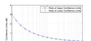
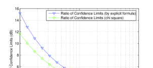
Figure 1: Plots of $20\log_{10}\left(\frac{1}{(1+\varepsilon)C_{1}}\right)$ and $20\log_{10}\left(\frac{1}{(1-\varepsilon)C_{2}}\right)$ (left), and $20\log_{10}\left(\frac{1+\varepsilon}{1-\varepsilon}\right)$ (right) vs. $N$

In summary our results on the sample complexity are quite satisfactory as demonstrated in Figure 1 that can in fact be extended to the noisy case.

4 Measurement and Estimation with Noisy Samples

Recall that in the noisy case two sets of i.i.d. BPSK symbols are transmitted with difference in their average power satisfying $P_{s1}>P_{s2}\geq 0$. The problem is statistical estimation for $\sigma_{H}^{2}$, $\sigma_{V}^{2}$, and the SNR, as well as their associated sample complexity bound based on i.i.d. observations of the received signal $X=HS+V$ which are recorded as $\{X_{1,i}\}_{i=1}^{N_{1}}$ and $\{X_{2,i}\}_{i=1}^{N_{2}}$, respectively. We consider the case where $N_{1}=N_{2}=N$ with $\overline{X_{1,N}^{2}}$ and $\overline{X_{2,N}^{2}}$ as defined in (6). Two different subjects will be investigated.

4.1 Interval Estimate

We will demonstrate not only how to construct a simultaneous confidence interval based on the noisy measurements but also how tight these interval estimates are. Our main results begin with the following theorem that provides a simultaneous interval estimate and the solution to the sample complexity problem with an a priori bound.

Theorem 3

Let $\varepsilon$ and $\delta$ be positive numbers less than $1$. Denote $\Delta P_{s}=P_{s1}-P_{s2}$. Then

$$\Pr\left\{\begin{array}[]{c}\hskip 17.07164pt\frac{1}{\Delta P_{s}}\left(\frac{\overline{X_{1,N}^{2}}}{1+\varepsilon}-\frac{\overline{X_{2,N}^{2}}}{1-\varepsilon}\right)<\sigma_{H}^{2}<\frac{1}{\Delta P_{s}}\left(\frac{\overline{X_{1,N}^{2}}}{1-\varepsilon}-\frac{\overline{X_{2,N}^{2}}}{1+\varepsilon}\right)\;\,\,\&\\ \frac{1}{\Delta P_{s}}\left(\frac{P_{s1}\overline{X_{2,N}^{2}}}{1+\varepsilon}-\frac{P_{s2}\overline{X_{1,N}^{2}}}{1-\varepsilon}\right)<\sigma_{V}^{2}<\frac{1}{\Delta P_{s}}\left(\frac{P_{s1}\overline{X_{2,N}^{2}}}{1-\varepsilon}-\frac{P_{s2}\overline{X_{1,N}^{2}}}{1+\varepsilon}\right)\end{array}\right\}>1-\delta$$ (21)

provided that $N>\frac{2(3+2\varepsilon)\ln(\frac{4}{\delta})}{3\varepsilon^{2}}$.

Proof. For BPSK the transmitted symbol $S$ is real with the transmitting power $P_{s}=|S|^{2}$, and thus

$$X=HS+V=(H_{R}S+V_{R})+j(H_{I}S+V_{I})=\sqrt{(P_{s}\sigma_{H}^{2}+\sigma_{V}^{2})}(A+jB)$$

where $A$ and $B$ are independent Gaussian variables with zero mean and unity variance. Hence $|X|^{2}=(P_{s}\sigma_{H}^{2}+\sigma_{V}^{2})(A^{2}+B^{2})$ is Rayleigh distributed. It follows that $\{X_{1,i}\}_{i=1}^{N}$ and $\{X_{2,i}\}_{i=1}^{N}$ are both i.i.d. observations of $X$, and with $\overline{X_{1,N}^{2}}$ and $\overline{X_{2,N}^{2}}$ as defined in (6),

$$\mathbb{E}\left[\overline{X_{\ell,N}^{2}}\right]=\left(P_{s_{\ell}}\sigma_{H}^{2}+\sigma_{V}^{2}\right),\;\;\;\;\;\ell=1,2$$

Applying (i) of Corollary 1 yields the interval estimate

$$\Pr\left\{\frac{\overline{X_{\ell,N}^{2}}}{1+\varepsilon}<(P_{s_{\ell}}\sigma_{H}^{2}+\sigma_{V}^{2})<\frac{\overline{X_{\ell,N}^{2}}}{1-\varepsilon}\right\}>\sqrt{1-\delta},\;\;\;\;\;\ell=1,2$$

for an appropriately chosen sample size $N$. In fact the above holds, if

$$N>\frac{2(3+2\varepsilon){\rm ln}\left(\frac{2}{1-\sqrt{1-\delta}}\right)}{3\varepsilon^{2}}$$ (22)

in light of Corollary 1. The fact that $(1-\sqrt{1-\delta})^{2}=2-\delta-2\sqrt{1-\delta}>0$ implies that $1-\sqrt{1-\delta}>\frac{\delta}{2}$. Hence the inequality in (22) holds provided that $N>\frac{2(3+2\varepsilon)\ln(\frac{4}{\delta})}{3\varepsilon^{2}}$ as in the statement of the theorem. Now by the independence of the experiment,

$$\Pr\left\{\frac{\overline{X_{1,N}^{2}}}{1+\varepsilon}<(P_{s1}\sigma_{H}^{2}+\sigma_{V}^{2})<\frac{\overline{X_{1,N}^{2}}}{1-\varepsilon},\;\;\;\frac{\overline{X_{2,N}^{2}}}{1+\varepsilon}<(P_{s2}\sigma_{H}^{2}+\sigma_{V}^{2})<\frac{\overline{X_{2,N}^{2}}}{1-\varepsilon}\right\}>1-\delta$$

Define the following sets of events as illustrated in Figure 2:

$${\mathcal{S}}_{0} = \left\{(\sigma_{H}^{2},\sigma_{V}^{2}):\;\;\mbox{the joint events in the probability expression (\ref{pr2}) hold}\right\}$$ (23)

$${\mathcal{S}}_{1} = \left\{(\sigma_{H}^{2},\sigma_{V}^{2}):\;\;\frac{\overline{X_{1,N}^{2}}}{1+\varepsilon}<(P_{s1}\sigma_{H}^{2}+\sigma_{V}^{2})<\frac{\overline{X_{1,N}^{2}}}{1-\varepsilon}\right\}$$ (24)

$${\mathcal{S}}_{2} = \left\{(\sigma_{H}^{2},\sigma_{V}^{2}):\;\;\frac{\overline{X_{2,N}^{2}}}{1+\varepsilon}<(P_{s2}\sigma_{H}^{2}+\sigma_{V}^{2})<\frac{\overline{X_{2,N}^{2}}}{1-\varepsilon}\right\}$$ (25)

We will show that ${\mathcal{S}}_{1}\cap{\mathcal{S}}_{2}\subseteq{\mathcal{S}}_{0}$ leading to $\Pr\{{\mathcal{S}}_{0}\}\geq\Pr\{{\mathcal{S}}_{1}\cap{\mathcal{S}}_{2}\}>1-\delta$ thereby concluding the proof.

Figure 2: Illustration of the sets of events

Indeed suppose that $(\sigma_{H}^{2},\sigma_{V}^{2})\in{\mathcal{S}}_{1}\cap{\mathcal{S}}_{2}$ represented by the shaded area in Figure 2. Then

$$\frac{\overline{X_{1,N}^{2}}}{1+\varepsilon}<(P_{s1}\sigma_{H}^{2}+\sigma_{V}^{2})<\frac{\overline{X_{1,N}^{2}}}{1-\varepsilon}\;\;\;\&\;\;\;-\frac{\overline{X_{2,N}^{2}}}{1-\varepsilon}<-(P_{s2}\sigma_{H}^{2}+\sigma_{V}^{2})<-\frac{\overline{X_{2,N}^{2}}}{1+\varepsilon}$$

The above inequalities can be combined to eliminate $\sigma_{V}^{2}$ yielding

$$(\sigma_{H}^{2},\sigma_{V}^{2})\in{\mathcal{S}}_{H}:=\left\{\sigma_{H}^{2}:\;\;\;\frac{1}{\Delta P_{s}}\left(\frac{\overline{X_{1,N}^{2}}}{1+\varepsilon}-\frac{\overline{X_{2,N}^{2}}}{1-\varepsilon}\right)<\sigma_{H}^{2}<\frac{1}{\Delta P_{s}}\left(\frac{\overline{X_{1,N}^{2}}}{1-\varepsilon}-\frac{\overline{X_{2,N}^{2}}}{1+\varepsilon}\right)\right\}$$ (26)

On the other hand for $(\sigma_{H}^{2},\sigma_{V}^{2})\in{\mathcal{S}}_{1}\cap{\mathcal{S}}_{2}$, there hold

$$\frac{P_{s1}\overline{X_{2,N}^{2}}}{1+\varepsilon}< (P_{s1}P_{s2}\sigma_{H}^{2}+P_{s1}\sigma_{V}^{2}) <\frac{P_{s1}\overline{X_{2,N}^{2}}}{1-\varepsilon}\;\;\;\&$$

$$-\frac{P_{s2}\overline{X_{1,N}^{2}}}{1-\varepsilon}< -(P_{s1}P_{s2}\sigma_{H}^{2}+P_{s2}\sigma_{V}^{2}) <-\frac{P_{s2}\overline{X_{1,N}^{2}}}{1+\varepsilon}$$

The above inequalities can be combined to eliminate $\sigma_{H}^{2}$ yielding $(\sigma_{H}^{2},\sigma_{V}^{2})\in{\mathcal{S}}_{V}$ with

$${\mathcal{S}}_{V}:=\left\{\sigma_{V}^{2}:\;\;\;\frac{1}{\Delta P_{s}}\left(\frac{P_{s1}\overline{X_{2,N}^{2}}}{1+\varepsilon}-\frac{P_{s2}\overline{X_{1,N}^{2}}}{1-\varepsilon}\right)<\sigma_{V}^{2}<\frac{1}{\Delta P_{s}}\left(\frac{P_{s1}\overline{X_{2,N}^{2}}}{1-\varepsilon}-\frac{P_{s2}\overline{X_{1,N}^{2}}}{1+\varepsilon}\right)\right\}$$ (27)

We can thus conclude that ${\mathcal{S}}_{1}\cap{\mathcal{S}}_{2}\subseteq{\mathcal{S}}_{0}={\mathcal{S}}_{H}\cap{\mathcal{S}}_{V}$ represented by the rectangular area in Figure 2. The proof is now complete. $\Box$

The proof of Theorem 3 shows that two signal sets of different strengths are necessary in order to resolve two different interval estimates for $\sigma_{H}^{2}$ and $\sigma_{V}^{2}$, respectively. Clearly signals of more than two different strengths become necessary in order to acquire more than two independent parameters in statistical estimation of wireless channels. Theorem 3 also shows that for $N>\frac{2(3+\varepsilon)\ln(\frac{4}{\delta})}{3\varepsilon^{2}}$,

$$\Pr\left\{{\mathcal{S}}_{H}\right\} = \Pr\left\{\frac{1}{\Delta P_{s}}\left(\frac{\overline{X_{1,N}^{2}}}{1+\varepsilon}-\frac{\overline{X_{2,N}^{2}}}{1-\varepsilon}\right)<\sigma_{H}^{2}<\frac{1}{\Delta P_{s}}\left(\frac{\overline{X_{1,N}^{2}}}{1-\varepsilon}-\frac{\overline{X_{2,N}^{2}}}{1+\varepsilon}\right)\right\}>1-\delta$$

$$\Pr\left\{{\mathcal{S}}_{V}\right\} = \Pr\left\{\frac{1}{\Delta P_{s}}\left(\frac{P_{s1}\overline{X_{2,N}^{2}}}{1+\varepsilon}-\frac{P_{s2}\overline{X_{1,N}^{2}}}{1-\varepsilon}\right)<\sigma_{V}^{2}<\frac{1}{\Delta P_{s}}\left(\frac{P_{s1}\overline{X_{2,N}^{2}}}{1-\varepsilon}-\frac{P_{s2}\overline{X_{1,N}^{2}}}{1+\varepsilon}\right)\right\}>1-\delta$$

Remark 4  In light of Remark 2 and the definition of $F_{\chi^{2},2N}(\cdot)$, the sample complexity bound in Theorem 3 can be improved by taking $N=N_{\rm m2}$, the minimum positive integer such that

$$F_{\chi^{2},2N_{\rm m2}}((1+\varepsilon)2N_{\rm m2})-F_{\chi^{2},2N_{\rm m2}}((1-\varepsilon)2N_{\rm m2})\geq\sqrt{1-\delta}$$ (28)

Recall that SNR $=10\log_{10}\mathbb{E}[|S|^{2}]+10\log_{10}\left(\frac{\sigma_{H}^{2}}{\sigma_{V}^{2}}\right)$, it is both important and of independent interest to obtain an interval estimate for $\frac{\sigma_{H}^{2}}{\sigma_{V}^{2}}$ that is presented in the next result.

Corollary 2

Let $\varepsilon$, $\delta$ be positive numbers less than $1$, and $P_{s2}=0$. Suppose that $N$ is the minimum positive integer such that $(\ref{nmin2})$ holds. Then,

$$\Pr\left\{\frac{1}{P_{s1}}\left(\frac{(1-\varepsilon)\overline{X_{1,N}^{2}}}{(1+\varepsilon)\overline{X_{2,N}^{2}}}-1\right)<\frac{\sigma_{H}^{2}}{\sigma_{V}^{2}}<\frac{1}{P_{s1}}\left(\frac{(1+\varepsilon)\overline{X_{1,N}^{2}}}{(1-\varepsilon)\overline{X_{2,N}^{2}}}-1\right)\right\}>1-\delta$$

Proof. In reference to the sets of the events as illustrated in Figure 2, the hypothesis $P_{s2}=0$ implies

$${\mathcal{S}}_{1}\cap{\mathcal{S}}_{2}=\left\{(\sigma_{H}^{2},\sigma_{V}^{2}):\;\;\;\frac{\overline{X_{1,N}^{2}}}{1+\varepsilon}<(P_{s1}\sigma_{H}^{2}+\sigma_{V}^{2})<\frac{\overline{X_{1,N}^{2}}}{1-\varepsilon}\;\;\&\;\;\frac{\overline{X_{2,N}^{2}}}{1+\varepsilon}<\sigma_{V}^{2}<\frac{\overline{X_{2,N}^{2}}}{1-\varepsilon}\right\}$$

Suppose that $(\sigma_{H}^{2},\sigma_{V}^{2})\in{\mathcal{S}}_{1}\cap{\mathcal{S}}_{2}$. Then some algebraic manipulations yield that

$$(\sigma_{H}^{2},\sigma_{V}^{2})\in{\mathcal{S}}_{H,V}:=\left\{(\sigma_{H}^{2},\sigma_{V}^{2}):\;\;\;\frac{(1-\varepsilon)\overline{X_{1,N}^{2}}}{(1+\varepsilon)\overline{X_{2,N}^{2}}}<\frac{P_{s1}\sigma_{H}^{2}}{\sigma_{V}^{2}}+1<\frac{(1+\varepsilon)\overline{X_{1,N}^{2}}}{(1-\varepsilon)\overline{X_{2,N}^{2}}}\right\}$$ (29)

As a result ${\mathcal{S}}_{1}\cap{\mathcal{S}}_{2}\subseteq{\mathcal{S}}_{H,V}$ and thus $\Pr\{{\mathcal{S}}_{H,V}\}\geq\Pr\{{\mathcal{S}}_{1}\cap{\mathcal{S}}_{2}\}\geq 1-\delta$, if $N$ satisfies the (28) by Remark 3. Therefore the corollary is true. $\Box$

In the case $P_{s2}\neq 0$, the result in Corollary 2 needs to be replaced by a more complex expression:

$$\Pr\left\{\frac{\left(1-\frac{P_{s2}}{P_{s1}}\right)\overline{X_{1,N}^{2}}}{\left(\frac{1+\varepsilon}{1-\varepsilon}\right)P_{s1}\overline{X_{2,N}^{2}}-P_{s2}\overline{X_{1,N}^{2}}}-\frac{1}{P_{s1}}<\frac{\sigma_{H}^{2}}{\sigma_{V}^{2}}<\frac{\left(1-\frac{P_{s2}}{P_{s1}}\right)\overline{X_{1,N}^{2}}}{\left(\frac{1-\varepsilon}{1+\varepsilon}\right)P_{s1}\overline{X_{2,N}^{2}}-P_{s2}\overline{X_{1,N}^{2}}}-\frac{1}{P_{s1}}\right\}>1-\delta$$ (30)

if the positive integer $N$ satisfies (28), and if $\left(\frac{1+\varepsilon}{1-\varepsilon}\right)P_{s1}\overline{X_{2,N}^{2}}-P_{s2}\overline{X_{1,N}^{2}}>0$ and $\left(\frac{1-\varepsilon}{1+\varepsilon}\right)P_{s1}\overline{X_{2,N}^{2}}-P_{s2}\overline{X_{1,N}^{2}}>0$. The above reduces to that of Corollary 2 in the case $P_{s2}=0$.

We investigate next whether or not the interval estimates presented in Theorem 3 and Corollary 2 are tight. Such an issue is clearly dependent on the average transmitting powers $P_{s1}$ and $P_{s2}$. Recall that $P_{s1}>P_{s2}\geq 0$. Intuitively the larger $P_{s1}$ and the smaller $P_{s2}$ are, the tighter the interval estimates are that is validated by the following result.

Theorem 4

Let $\varepsilon$, $\delta$ be positive numbers less than $1$, and $N=N_{\rm m2}-1\geq N_{\rm m1}$ with $N_{\rm m1}$ and $N_{\rm m2}$ the minimum positive integers satisfying $(\ref{nmin1})$ and $(\ref{nmin2})$, respectively. Then

$$1-\delta\leq\Pr\left\{\frac{1}{\Delta P_{s}}\left(\frac{\overline{X_{1,N}^{2}}}{1+\varepsilon}-\frac{\overline{X_{2,N}^{2}}}{1-\varepsilon}\right)<\sigma_{H}^{2}<\frac{1}{\Delta P_{s}}\left(\frac{\overline{X_{1,N}^{2}}}{1-\varepsilon}-\frac{\overline{X_{2,N}^{2}}}{1+\varepsilon}\right)\right\}<1-\frac{\delta}{2}$$ (31)

for sufficiently large $P_{s1}$ with constant $P_{s2}$. In addition

$$1-\delta\leq\Pr\left\{\frac{1}{\Delta P_{s}}\left(\frac{P_{s1}\overline{X_{2,N}^{2}}}{1+\varepsilon}-\frac{P_{s2}\overline{X_{1,N}^{2}}}{1-\varepsilon}\right)<\sigma_{V}^{2}<\frac{1}{\Delta P_{s}}\left(\frac{P_{s1}\overline{X_{2,N}^{2}}}{1-\varepsilon}-\frac{P_{s2}\overline{X_{1,N}^{2}}}{1+\varepsilon}\right)\right\}<1-\frac{\delta}{2}$$ (32)

for sufficiently small $P_{s2}$ with constant $P_{s1}$. Finally $1-\frac{\delta}{2}$ is also an upper bound for the confidence level in Theorem 3 and Corollary 2 with sufficiently large $P_{s1}$ and sufficiently small $P_{s2}$, if $N=N_{\rm m2}-1$.

Proof. In light of Remark 4 and the hypothesis on $N$, there holds

$$\sqrt{1-\delta} \geq \Pr\left\{\frac{\overline{X_{1,N}^{2}}}{1+\varepsilon}<(P_{s1}\sigma_{H}^{2}+\sigma_{V}^{2})<\frac{\overline{X_{1,N}^{2}}}{1-\varepsilon}\right\}$$

$$= \Pr\left\{(1-\varepsilon)(P_{s1}\sigma_{H}^{2}+\sigma_{V}^{2})<\overline{X_{1,N}^{2}}<(1+\varepsilon)(P_{s1}\sigma_{H}^{2}+\sigma_{V}^{2})\right\}$$

$$= \Pr\left\{(1-\varepsilon)\left(\sigma_{H}^{2}+\frac{\sigma_{V}^{2}}{P_{s1}}\right)<\frac{\overline{X_{1,N}^{2}}}{P_{s1}}<(1+\varepsilon)\left(\sigma_{H}^{2}+\frac{\sigma_{V}^{2}}{P_{s1}}\right)\right\}$$

$$\rightarrow \Pr\left\{(1-\varepsilon)\sigma_{H}^{2}<\widehat{\sigma}_{H,N}^{2,(\infty)}<(1+\varepsilon)\sigma_{H}^{2}\right\}>1-\delta$$

where $\widehat{\sigma}_{H,N}^{2,(\infty)}$ is the limit of $\widehat{\sigma}_{H,N}^{2}$, a point estimate for $\sigma^{2}_{H}$ to be investigated later:

$$\widehat{\sigma}_{H,N}^{2,(\infty)}=\lim_{P_{s1}\rightarrow\infty}\frac{\overline{X_{1,N}^{2}}}{P_{s1}}=\lim_{P_{s1}\rightarrow\infty}\left\{\widehat{\sigma}_{H,N}^{2}:=\frac{\overline{X_{1,N}^{2}}-\overline{X_{2,N}^{2}}}{P_{s1}-P_{s2}}\right\}$$ (33)

The last inequality follows from the hypothesis on $N_{\rm m2}>N_{\rm m1}$ and from the fact that $P_{s1}\rightarrow\infty$ corresponds to the noise-free case in Section 3. Recall ${\mathcal{S}}_{H}$ as defined in (26) that can be alternatively described as

$${\mathcal{S}}_{H}=\left\{\sigma_{H}^{2}:\;\;\delta P_{s}(1-\varepsilon)\sigma_{H}^{2}+\frac{(1-\varepsilon)\overline{X_{2,N}^{2}}}{(1+\varepsilon)P_{s1}}<\frac{\overline{X_{1,N}^{2}}}{P_{s1}}<\delta P_{s}(1+\varepsilon)\sigma_{H}^{2}+\frac{(1+\varepsilon)\overline{X_{2,N}^{2}}}{(1-\varepsilon)P_{s1}}\right\}$$ (34)

where $\delta P_{s}=\left(1-\frac{P_{s2}}{P_{s1}}\right)$. It is easy to see that as $P_{s1}\rightarrow\infty$,

$$\Pr\left\{{\mathcal{S}}_{H}\right\}\rightarrow\Pr\left\{(1-\varepsilon)\sigma_{H}^{2}<\widehat{\sigma}_{H,N}^{2,(\infty)}<(1+\varepsilon)\sigma_{H}^{2}\right\}>1-\delta$$

It follows that the lower bound in (31) is true by taking $P_{s1}$ sufficiently large. On the other hand

$$\Pr\left\{{\mathcal{S}}_{H}\right\}\rightarrow\Pr\left\{(1-\varepsilon)\sigma_{H}^{2}<\widehat{\sigma}_{H,N}^{2,(\infty)}<(1+\varepsilon)\sigma_{H}^{2}\right\}\leq\sqrt{1-\delta}$$

It follows that there exists $P_{s1}>0$ such that

$$\Pr\left\{{\mathcal{S}}_{H}\right\}<\sqrt{1-\delta}+\frac{1}{2}\left(1-\sqrt{1-\delta}\right)^{2}=1-\frac{\delta}{2}$$

provided that $P_{s1}$ is large enough that concludes the upper bound in (31). The proof for (32) is similar. Indeed by applying the result from the previous section and using the hypothesis $N_{\rm m1}<N_{\rm m2}$,

$$\sqrt{1-\delta} \geq \Pr\left\{\frac{\overline{X_{2,N}^{2}}}{1+\varepsilon}<(P_{s2}\sigma_{H}^{2}+\sigma_{V}^{2})<\frac{\overline{X_{2,N}^{2}}}{1-\varepsilon}\right\}$$

$$= \Pr\left\{(1-\varepsilon)(P_{s2}\sigma_{H}^{2}+\sigma_{V}^{2})<\overline{X_{2,N}^{2}}<(1+\varepsilon)(P_{s2}\sigma_{H}^{2}+\sigma_{V}^{2})\right\}$$

$$\rightarrow \Pr\left\{(1-\varepsilon)\sigma_{V}^{2}<\overline{X_{2,N}^{2}}<(1+\varepsilon)\sigma_{V}^{2}\right\}>1-\delta$$

as $P_{s2}\rightarrow 0$. Recall ${\mathcal{S}}_{V}$ as defined in (27). Then

$$1-\frac{\delta}{2}>\sqrt{1-\delta}\geq\lim_{P_{s2}\rightarrow 0}\Pr\{{\mathcal{S}}_{V}\}=\Pr\left\{(1-\varepsilon)\sigma_{V}^{2}<\overline{X_{2,N}^{2}}<(1+\varepsilon)\sigma_{V}^{2}\right\}>1-\delta$$

It follows that both lower and upper bounds in (32) are true by taking $P_{s2}>0$ sufficiently close to 0. Finally the proofs for the rest of the theorem are omitted because they are similar to those for the lower bounds in (31) and (32). $\Box$

Remark 5  Theorem 4 shows that the conservativeness of the coverage probability can be controlled within $\frac{\delta}{2}$. Since the experimental effort grows in the order of $\ln(\frac{2}{\delta})$ for a fixed relative width of the confidence interval, a gain of $\frac{\delta}{2}$ for the coverage probability can be obtained at the cost of increasing the experimental effort by

$$100\left(\frac{\ln\left(\frac{2}{\delta/2}\right)}{\ln\left(\frac{2}{\delta}\right)}-1\right)\%=\frac{100\ln(2)}{\ln\left(\frac{2}{\delta}\right)}\%$$

It can be seen that this percentage is very insignificant for small $\delta$. Therefore, the conservativeness of the proposed interval estimation can be made very insignificant by choosing large $P_{s1}$ and small $P_{s2}$.

The hypothesis $N_{\rm m2}>N_{\rm m1}$ in Theorem 4 is generically true for small $\delta$ and $\varepsilon$ in light of the fact that $N_{\rm m2}\ln\left(\frac{2}{\delta}\right)\approx N_{\rm m1}\ln\left(\frac{4}{\delta}\right)$. Because the limiting case $P_{s1}\rightarrow\infty$ is equivalent to the noiseless case, there hold

$$\lim_{P_{s1}\rightarrow\infty}\Pr\left\{\frac{\overline{X_{1,N}^{2}}}{(1+\varepsilon)P_{s1}}<\sigma_{H}^{2}<\frac{\overline{X_{1,N}^{2}}}{(1-\varepsilon)P_{s1}}\right\}>1-\delta,\;\;\;\;\;\lim_{P_{s1}\rightarrow\infty\atop{P_{s2}\rightarrow 0}}\Pr\left\{\frac{\overline{X_{2,N}^{2}}}{1+\varepsilon}<\sigma_{V}^{2}<\frac{\overline{X_{2,N}^{2}}}{1-\varepsilon}\right\}>1-\delta$$

provided that $N>\frac{2(3+2\varepsilon)\ln(\frac{2}{\delta})}{3\varepsilon^{2}}\geq N_{\rm m1}$ where $\varepsilon$ and $\delta$ are positive numbers less than 1. The sample complexity bound for the limiting case improves the one in Theorem 4.

4.2 Point Estimate

In light of the results in [13], $\overline{X_{\ell,N}^{2}}$ ($\ell=1$ or $\ell=2$) is the ML estimator for $P_{s\ell}\sigma_{H}^{2}+\sigma_{V}^{2}$ that is both sufficient and complete statistic. Let $\widehat{\sigma}_{H,N}^{2}$ and $\widehat{\sigma}_{V,N}^{2}$ be point estimates for $\sigma_{H}^{2}$ and $\sigma_{V}^{2}$, respectively based on $\overline{X_{1,N}^{2}}$ and $\overline{X_{2,N}^{2}}$. Then

$$P_{s1}\widehat{\sigma}_{H,N}^{2}+\widehat{\sigma}_{V,N}^{2}=\overline{X_{1,N}^{2}},\;\;\;\;\;P_{s2}\widehat{\sigma}_{H,N}^{2}+\widehat{\sigma}_{V,N}^{2}=\overline{X_{2,N}^{2}}$$ (35)

giving rise to the following expressions for the point estimates (recall $\Delta P_{s}=P_{s1}-P_{s2}>0$):

$$\widehat{\sigma}_{H,N}^{2}=\frac{1}{\Delta P_{s}}\left(\overline{X_{1,N}^{2}}-\overline{X_{2,N}^{2}}\right),\;\;\;\;\;\widehat{\sigma}_{V,N}^{2}=\frac{1}{\Delta P_{s}}\left(P_{s1}\overline{X_{2,N}^{2}}-P_{s2}\overline{X_{1,N}^{2}}\right)$$ (36)

Our next result shows that both $\widehat{\sigma}_{H,N}^{2}$ and $\widehat{\sigma}_{V,N}^{2}$ are optimum estimators for $\sigma_{H}^{2}$ and $\sigma_{V}^{2}$, respectively.

Theorem 5

Let $\{X_{1,k}\}_{k=1}^{N}$ and $\{X_{2,k}\}_{k=1}^{N}$ be $2N$ i.i.d. noisy samples with $P_{s1}>P_{s2}\geq 0$. Then $\widehat{\sigma}_{H,N}^{2}$ and $\widehat{\sigma}_{V,N}^{2}$ as in $(\ref{est})$ are unbiased ML and MV estimates for $\sigma_{H}^{2}$ and $\sigma_{V}^{2}$, respectively that achieve the Cramér-Rao lower bound. Furthermore $\overline{X_{1,N}^{2}}$ and $\overline{X_{2,N}^{2}}$ as in $(\ref{tmp0})$ are sufficient and complete statistics.

Proof. It can be easily verified that $\mathbb{E}[\overline{X_{\ell,N}^{2}}]=P_{s\ell}\sigma_{H}^{2}+\sigma_{V}^{2}$ for $\ell=1,2$ implying that $\mathbb{E}[\widehat{\sigma}_{H,N}^{2}]=\sigma_{H}^{2}$ and $\mathbb{E}[\widehat{\sigma}_{V,N}^{2}]=\sigma_{V}^{2}$. Thus the estimator in $(\ref{est})$ is unbiased. By independence the joint PDF for $\{X_{1,k}\}_{k=1}^{N}$ and $\{X_{2,k}\}_{k=1}^{N}$ is given by

$$f_{X}\left(\{X_{1,k}\}_{k=1}^{N},\{X_{2,k}\}_{k=1}^{N}\right)=f_{X}\left(\{X_{1,k}\}_{k=1}^{N}\right)f_{X}\left(\{X_{2,k}\}_{k=1}^{N}\right)$$ (37)

by an abuse of notation where for either $\ell=1$ or $\ell=2$,

$$f_{X}\left(\{X_{\ell,k}\}_{k=1}^{N}\right)=\frac{1}{(P_{s\ell}\sigma_{H}^{2}+\sigma_{V}^{2})^{N}}{\rm exp}\left\{\sum_{i=1}^{N}\ln(|X_{\ell,i}|)\right\}{\rm exp}\left\{-\frac{N\overline{X_{\ell,N}^{2}}}{P_{s\ell}\sigma_{H}^{2}+\sigma_{V}^{2}}\right\}$$

Taking natural logarithm on both sides yields

$$\ln(f_{X})=-\ln(P_{s1}\sigma_{H}^{2}+\sigma_{V}^{2})^{N}-\ln(P_{s2}\sigma_{H}^{2}+\sigma_{V}^{2})^{N}+\sum_{i=1}^{N}\ln(|X_{1,i}X_{2,i}|)-\frac{N\overline{X_{1,N}^{2}}}{P_{s1}\sigma_{H}^{2}+\sigma_{V}^{2}}-\frac{N\overline{X_{2,N}^{2}}}{P_{s2}\sigma_{H}^{2}+\sigma_{V}^{2}}$$

Setting partial derivatives of $\ln(f_{X})$ with respect to $\sigma_{H}^{2}$ and $\sigma_{V}^{2}$ to zeros lead to the following two equations:

$$\frac{P_{s1}\overline{X_{1,N}^{2}}}{(P_{s1}\sigma_{H}^{2}+\sigma_{V}^{2})^{2}}+\frac{P_{s2}\overline{X_{2,N}^{2}}}{(P_{s2}\sigma_{H}^{2}+\sigma_{V}^{2})^{2}} = \frac{P_{s1}}{P_{s1}\sigma_{H}^{2}+\sigma_{V}^{2}}+\frac{P_{s2}}{P_{s2}\sigma_{H}^{2}+\sigma_{V}^{2}}$$

$$\frac{\overline{X_{1,N}^{2}}}{(P_{s1}\sigma_{H}^{2}+\sigma_{V}^{2})^{2}}+\frac{\overline{X_{2,N}^{2}}}{(P_{s2}\sigma_{H}^{2}+\sigma_{V}^{2})^{2}} = \frac{1}{P_{s1}\sigma_{H}^{2}+\sigma_{V}^{2}}+\frac{1}{P_{s2}\sigma_{H}^{2}+\sigma_{V}^{2}}$$

Solving for $\overline{X_{1,N}^{2}}$ and $\overline{X_{2,N}^{2}}$ from the above two equations coincide with the expressions in (35) at $\sigma_{H}^{2}=\widehat{\sigma}_{H,N}^{2}$ and $\sigma_{V}^{2}=\widehat{\sigma}_{V,N}^{2}$ that in turn gives the point estimates in (36). The uniqueness of the solution implies that the points estimates in (36) are indeed ML that maximize the PDF $f_{X}(\cdot)$ for every pair of sets of $N$ i.i.d. noisy measurement samples satisfying the hypothesis. Denote $\theta=\left[\begin{array}[]{cc}\sigma_{H}^{2}&\sigma_{V}^{2}\end{array}\right]^{T}$ as the parameter vector for estimation where superscript ^T denotes transpose. Then the corresponding FIM (Fisher information matrix) can be shown to be, after lengthy calculation,

$${\rm Fim}(\sigma_{H}^{2},\sigma_{V}^{2}):=\mathbb{E}\left\{\left[\frac{\partial\ln(f_{X})}{\partial\theta}\right]\left[\frac{\partial\ln(f_{X})}{\partial\theta}\right]^{T}\right\}=N\left[\begin{array}[]{cc}\frac{P_{s1}^{2}}{\sigma_{1}^{4}}+\frac{P_{s2}^{2}}{\sigma_{2}^{4}}&\frac{P_{s1}}{\sigma_{1}^{4}}+\frac{P_{s2}}{\sigma_{2}^{4}}\\ \frac{P_{s1}}{\sigma_{1}^{4}}+\frac{P_{s2}}{\sigma_{2}^{4}}&\frac{1}{\sigma_{1}^{4}}+\frac{1}{\sigma_{2}^{4}}\end{array}\right]$$

where for simplicity in notations, $\sigma_{\ell}=P_{s\ell}\sigma_{H}^{2}+\sigma_{V}^{2}$ is used with $\ell=1,2$. Recall that the inverse of ${\rm Fim}(\sigma_{H}^{2},\sigma_{V}^{2})$ is the smallest error covariance achievable by all unbiased estimators. In arriving to the above expression, the fact that $\mathbb{E}[G^{4}]=3\sigma^{4}$ for $G$ distributed as $\mathscr{N}(0,\sigma)$, and the observations:

$$\mathbb{E}\left[\overline{X_{\ell,N}^{2}}\right] = P_{s\ell}\sigma_{H}^{2}+\sigma_{V}^{2},\;\;\;\;\;\mathbb{E}\left[(\overline{X_{1,N}^{2}})(\overline{X_{2,N}^{2}})\right]=(P_{s1}\sigma_{H}^{2}+\sigma_{V}^{2})(P_{s2}\sigma_{H}^{2}+\sigma_{V}^{2})$$

$$\mathbb{E}\left[\left(\overline{X_{\ell,N}^{2}}\right)^{2}\right] = (P_{s\ell}\sigma_{H}^{2}+\sigma_{V}^{2})^{2}+\frac{1}{N}(P_{s\ell}\sigma_{H}^{2}+\sigma_{V}^{2})^{2},\;\;\;\;\;\ell=1,2$$

are crucial. Now with the point estimates in (36), the corresponding error covariance can be shown to be

$${\rm Cov}(\sigma_{H}^{2},\sigma_{V}^{2}) = \mathbb{E}\left\{\left[\begin{array}[]{c}\widehat{\sigma}_{H,N}^{2}-\sigma_{H}^{2}\\ \widehat{\sigma}_{V,N}^{2}-\sigma_{V}^{2}\end{array}\right]\left[\begin{array}[]{cc}\widehat{\sigma}_{H,N}^{2}-\sigma_{H}^{2}&\widehat{\sigma}_{V,N}^{2}-\sigma_{V}^{2}\end{array}\right]\right\}$$

$$= \frac{1}{N\Delta P_{s}}\left[\begin{array}[]{cc}\sigma_{1}^{4}+\sigma_{2}^{4}&-(P_{s1}\sigma_{2}^{4}+P_{s2}\sigma_{1}^{4})\\ -(P_{s1}\sigma_{2}^{4}+P_{s2}\sigma_{1}^{4})&P_{s1}^{2}\sigma_{2}^{4}+P_{s2}^{2}\sigma_{1}^{4}\end{array}\right]$$

where again the notation $\sigma_{\ell}^{2}=P_{s\ell}\sigma_{H}^{2}+\sigma_{V}^{2}$ with $\ell=1,2$ is used. Consequently there holds the identity ${\rm Fim}(\sigma_{H}^{2},\sigma_{V}^{2}){\rm Cov}(\sigma_{H}^{2},\sigma_{V}^{2})=I$, validating the fact that the Cramér-Rao lower bound is indeed achieved by the point estimates in (36) that are indeed MV estimates. Finally the sufficient and complete statistic of $\overline{X_{1,N}^{2}}$ and $\overline{X_{2,N}^{2}}$ can be shown in the same way as in [13]. Specifically the joint PDF in (37) has the form

$$f_{X}=g\left(\overline{X_{1,N}^{2}},\overline{X_{2,N}^{2}},\sigma_{H}^{2},\sigma_{V}^{2}\right)h\left(\{X_{1,k}\}_{k=1}^{N},\{X_{2,k}\}_{k=1}^{N}\right),\;\;\;\;\;h(\cdot,\cdot)=\prod_{i=1}^{N}|X_{1,i}X_{2,i}|$$

Hence in light of the Neyman factorization criterion, $\overline{X_{1,N}^{2}}$ and $\overline{X_{2,N}^{2}}$ are sufficient statistics. The proof for the complete statistics is again the same as that in [13] that is skipped. $\Box$

The result on the Cramér-Rao lower bound for finite $N$ in Theorem 5 is surprising which is normally achievable only asymptotically. Next we present several results for the point estimates in (36) regarding the sample complexity bound. We begin with a corollary that follows from the results on interval estimates in Subsection 4.1.

Corollary 3

Under the same hypotheses as in Theorem 4, there holds

$$1-\delta\leq\Pr\left\{\left|\frac{\widehat{\sigma}_{H,N}^{2}-\sigma_{H}^{2}}{\sigma_{H}^{2}}\right|<\varepsilon\right\}<1-\frac{\delta}{2}$$ (40)

for sufficiently large $P_{s1}$ with constant $P_{s2}$. In addition

$$1-\delta\leq\Pr\left\{\left|\frac{\widehat{\sigma}_{V,N}^{2}-\sigma_{V}^{2}}{\sigma_{V}^{2}}\right|<\varepsilon\right\}<1-\frac{\delta}{2}$$ (41)

for sufficiently small $P_{s2}$ with constant $P_{s1}$.

Proof. We prove only (40) as the proof for (41) is similar that will be omitted. Define the set of events:

$$\widehat{\mathcal{S}}_{H}:=\left\{\sigma_{H}^{2}:\;\;\frac{1}{\Delta P_{s}(1+\varepsilon)}\left(\overline{X_{1,N}^{2}}-\overline{X_{2,N}^{2}}\right)<\sigma_{H}^{2}<\frac{1}{\Delta P_{s}(1-\varepsilon)}\left(\overline{X_{1,N}^{2}}-\overline{X_{2,N}^{2}}\right)\right\}$$

Then $\widehat{\mathcal{S}}_{H}\subseteq{\mathcal{S}}_{H}$, and thus $\Pr\{\widehat{\mathcal{S}}_{H}\}\leq\Pr\{{\mathcal{S}}_{H}\}$. More importantly $\widehat{\mathcal{S}}_{H}\rightarrow{\mathcal{S}}_{H}$ as $P_{s1}\rightarrow\infty$. Therefore

$$\Pr\{\widehat{\mathcal{S}}_{H}\}=\Pr\left\{\frac{\widehat{\sigma}_{H,N}^{2}}{1+\varepsilon}<\sigma_{H}^{2}<\frac{\widehat{\sigma}_{H,N}^{2}}{1-\varepsilon}\right\}\\ =\Pr\left\{\left|\frac{\widehat{\sigma}_{H,N}^{2}-\sigma_{H}^{2}}{\sigma_{H}^{2}}\right|<\varepsilon\right\}\ \rightarrow\ \Pr\{{\mathcal{S}}_{H}\}$$

as $P_{s1}\rightarrow\infty$. A similar argument as in the proof of Theorem 4 can thus be used to conclude (40). $\Box$

Similar to the discussion after Remark 5, we have that for $N>\frac{2(3+2\varepsilon)\ln\frac{2}{\delta}}{3\varepsilon^{2}}$, there hold

$$\lim_{P_{s1}\to\infty}\Pr\left\{\left|\frac{\widehat{\sigma}_{H,N}^{2}-\sigma_{H}^{2}}{\sigma_{H}^{2}}\right|<\varepsilon\right\}>1-\delta\;\;\;\;\;\lim_{P_{s2}\to 0}\Pr\left\{\left|\frac{\widehat{\sigma}_{V,N}^{2}-\sigma_{V}^{2}}{\sigma_{V}^{2}}\right|<\varepsilon\right\}>1-\delta$$ (42)

where $\varepsilon$ and $\delta$ are positive numbers less than $1$. The next result is concerned with the point estimate related to SNR:

$$\widehat{\sigma}_{\frac{H}{V},N}^{2}=\frac{\widehat{\sigma}_{H,N}^{2}}{\widehat{\sigma}_{V,N}^{2}}=\frac{\overline{X_{1,N}^{2}}-\overline{X_{2,N}^{2}}}{P_{s1}\overline{X_{2,N}^{2}}-P_{s2}\overline{X_{1,N}^{2}}}$$ (43)

Theorem 6

Let $\varepsilon$ and $\delta$ be positive numbers less than $1$. Let $P_{s2}=0$. Suppose that $N$ is the minimum positive integer such that $F_{\chi^{2},2N}\left(2N(1+\frac{\varepsilon}{2+\varepsilon})\right)-F_{\chi^{2},2N}\left(2N(1-\frac{\varepsilon}{2+\varepsilon})\right)\geq\sqrt{1-\delta}$ where $F_{\chi^{2},2N}(\cdot)$ denotes the CDF of $\chi^{2}$ random variable with $2N$ degrees of freedom. Then

$$\lim_{P_{s1}\to\infty}\Pr\left\{\left|\frac{\widehat{\sigma}_{\frac{H}{V},N}^{2}-\frac{\sigma_{H}^{2}}{\sigma_{V}^{2}}}{\frac{\sigma_{H}^{2}}{\sigma_{V}^{2}}}\right|<\varepsilon\right\}>1-\delta$$

Proof. Define two normalized random variables by

$$\widehat{\theta}_{H,N}:=\frac{\overline{X_{1,N}^{2}}}{P_{s1}\sigma_{H}^{2}+\sigma_{V}^{2}},\;\;\;\;\;\widehat{\theta}_{V,N}:=\frac{\overline{X_{2,N}^{2}}}{\sigma_{V}^{2}}$$ (44)

Straightforward algebraic manipulations give the following chain of equations:

$$\Pr\left\{\left|\frac{\widehat{\sigma}_{\frac{H}{V},N}^{2}-\frac{\sigma_{H}^{2}}{\sigma_{V}^{2}}}{\frac{\sigma_{H}^{2}}{\sigma_{V}^{2}}}\right|<\varepsilon\right\} = \Pr\left\{\frac{\widehat{\sigma}_{\frac{H}{V},N}^{2}}{1+\varepsilon}<\frac{\sigma_{H}^{2}}{\sigma_{V}^{2}}<\frac{\widehat{\sigma}_{\frac{H}{V},N}^{2}}{1-\varepsilon}\right\}$$

$$= \Pr\left\{\frac{1}{P_{s1}(1+\varepsilon)}\left(\frac{\overline{X_{1,N}^{2}}}{\overline{X_{2,N}^{2}}}-1\right)<\frac{\sigma_{H}^{2}}{\sigma_{V}^{2}}<\frac{1}{P_{s1}(1-\varepsilon)}\left(\frac{\overline{X_{1,N}^{2}}}{\overline{X_{2,N}^{2}}}-1\right)\right\}$$

$$= \Pr\left\{\left(\frac{P_{s1}(1-\varepsilon)\sigma_{H}^{2}}{\sigma_{V}^{2}}+1\right)<\frac{\overline{X_{1,N}^{2}}}{\overline{X_{2,N}^{2}}}<\left(\frac{P_{s1}(1+\varepsilon)\sigma_{H}^{2}}{\sigma_{V}^{2}}+1\right)\right\}$$

$$= \Pr\left\{\frac{P_{s1}(1-\varepsilon)\sigma_{H}^{2}+\sigma_{V}^{2}}{P_{s1}\sigma_{H}^{2}+\sigma_{V}^{2}}<\frac{\widehat{\theta}_{H,N}}{\widehat{\theta}_{V,N}}<\frac{P_{s1}(1+\varepsilon)\sigma_{H}^{2}+\sigma_{V}^{2}}{P_{s1}\sigma_{H}^{2}+\sigma_{V}^{2}}\right\}$$

$$\rightarrow \Pr\left\{1-\varepsilon<\frac{\widehat{\theta}_{H,N}}{\widehat{\theta}_{V,N}}<1+\varepsilon\right\}$$

as $P_{s1}\rightarrow\infty$. To complete the proof, define two sets of events as follows:

$${\mathcal{S}}_{\theta} := \left\{(\widehat{\theta}_{H,N},\widehat{\theta}_{V,N}):\;\;\;(1-\varepsilon)\widehat{\theta}_{V,N}<\widehat{\theta}_{H,N}<(1+\varepsilon)\widehat{\theta}_{V,N}\right\},\;\;\;\;\;g(\varepsilon):=\frac{\varepsilon}{2+\varepsilon}$$

$$\widehat{\mathcal{S}}_{\theta} := \left\{(\widehat{\theta}_{H,N},\widehat{\theta}_{V,N}):\;\;\;1-g(\varepsilon)<\widehat{\theta}_{H,N}<1+g(\varepsilon)\;\;\;\&\;\;\;1-g(\varepsilon)<\widehat{\theta}_{V,N}<1+g(\varepsilon)\right\}$$

It can be shown that $\widehat{\mathcal{S}}_{\theta}\subseteq{\mathcal{S}}_{\theta}$. Indeed in the plane of $(\widehat{\theta}_{H,N},\widehat{\theta}_{V,N})$, the set $\widehat{\mathcal{S}}_{\theta}$ defines a square area inside the sector area defined by the set ${\mathcal{S}}_{\theta}$. More specifically

$$\widehat{\mathcal{S}}_{\theta}\subseteq\left\{(\widehat{\theta}_{H,N},\widehat{\theta}_{V,N}):\;\;\;1-\frac{\varepsilon}{2-\varepsilon}<\widehat{\theta}_{H,N}<1+g(\varepsilon)\;\;\;\&\;\;\;1-g(\varepsilon)<\widehat{\theta}_{V,N}<1+\frac{\varepsilon}{2-\varepsilon}\right\}\subseteq{\mathcal{S}}_{\theta}$$

It follows that as $P_{s1}\rightarrow\infty$, there holds

$$\Pr\{{\mathcal{S}}_{\theta}\} = \Pr\left\{1-\varepsilon<\frac{\widehat{\theta}_{H,N}}{\widehat{\theta}_{V,N}}<1+\varepsilon\right\}\geq\Pr\{\widehat{\mathcal{S}}_{\theta}\}$$

$$= \Pr\left\{1-g(\varepsilon)<\widehat{\theta}_{H,N}<1+g(\varepsilon)\right\}\Pr\left\{1-g(\varepsilon)<\widehat{\theta}_{V,N}<1+g(\varepsilon)\right\}>1-\delta$$

by independence of the events of $\widehat{\theta}_{H,N}$ and $\widehat{\theta}_{H,N}$, and by the hypothesis on $N$. $\Box$

By noting that $F_{\chi^{2},2N}\left(2N(1+\frac{\varepsilon}{2+\varepsilon})\right)-F_{\chi^{2},2N}\left(2N(1-\frac{\varepsilon}{2+\varepsilon})\right)\geq\sqrt{1-\delta}$, if $N>\frac{2(2+\varepsilon)(6+5\varepsilon)\ln\frac{4}{\delta}}{3\varepsilon^{2}}$, the next result follows from Theorem 6.

Corollary 4

Let $\varepsilon$ and $\delta$ be positive numbers less than $1$. Suppose that $P_{s2}=0$. Then

$$\lim_{P_{s1}\to\infty}\Pr\left\{\left|\frac{\widehat{\sigma}_{\frac{H}{V},N}^{2}-\frac{\sigma_{H}^{2}}{\sigma_{V}^{2}}}{\frac{\sigma_{H}^{2}}{\sigma_{V}^{2}}}\right|<\varepsilon\right\}>1-\delta$$

provided that $N>\frac{2(2+\varepsilon)(6+5\varepsilon)\ln\frac{4}{\delta}}{3\varepsilon^{2}}\approx\frac{8\ln(\frac{4}{\delta})}{\varepsilon^{2}}$ for small $\varepsilon$.

We note that $\frac{2(2+\varepsilon)(6+5\varepsilon)\ln\frac{4}{\delta}}{3\varepsilon^{2}}\approx\frac{8\ln(\frac{4}{\delta})}{\varepsilon^{2}}$ for small $\varepsilon$. Thus the a priori bounds for the sample complexity in Theorem 6 and Corollary 4 are roughly 4 times to that in Corollary 3. It signifies the difficulty in estimation of SNR in Rayleigh channels, and indicates that the margin of error manifested by $\varepsilon$ is more expensive to reduce as compared with the level of confidence manifested by $\delta$.

5 Numerical Simulations

This section presents numerical results to illustrate our proposed statistical theory in measurements and estimation of Rayleigh fading channels. For simplicity $\sigma_{H}^{2}=1$ and $P_{s1}=1$ are assumed throughout the section that can always be made true by a suitable normalization. Hence the SNR is the same as $\frac{\sigma_{H}^{2}}{\sigma_{V}^{2}}$, and large $P_{s1}$ reduces to large SNR. Moreover we consider only the case $P_{s2}=0$.

Because the noiseless case has been shown in Figure 1, we begin with the noisy measurement samples under SNR $=$ 20 dB by generating $\{X_{1,i}\}_{i=1}^{N}$ and $\{X_{2,i}\}_{i=1}^{N}$ for different sample size $N$. The simple averages $\overline{X_{\ell,N}^{2}}$ as in (6) are then calculated for $\ell=1,2$. We choose $\delta=0.01$ for the associated confidence level. In light of Theorem 3, there holds the joint probability

$$\Pr\left\{A_{1}<\sigma_{H}^{2}<A_{2}\;\&\;B_{1}<\sigma_{V}^{2}<B_{2}\right\}>1-\delta$$

where $A_{1},A_{2},B_{1},B_{2}$ are functions of $\varepsilon$, $N$, and $\overline{X_{\ell,N}^{2}}$ for $\ell=1,2$ which represent the interval estimates. In Figure 3 we plotted the ratios

$$\frac{A_{2}}{A_{1}}=\frac{(1+\varepsilon)\overline{X_{1,N}^{2}}-(1-\varepsilon)\overline{X_{2,N}^{2}}}{(1-\varepsilon)\overline{X_{1,N}^{2}}-(1+\varepsilon)\overline{X_{2,N}^{2}}},\;\;\;\;\;\;\;\frac{B_{2}}{B_{1}}=\frac{P_{s1}(1+\varepsilon)\overline{X_{2,N}^{2}}-P_{s2}(1-\varepsilon)\overline{X_{1,N}^{2}}}{P_{s1}(1-\varepsilon)\overline{X_{2,N}^{2}}-P_{s2}(1+\varepsilon)\overline{X_{1,N}^{2}}}$$

for the case $P_{s2}=0$ with SNR $=$ 20 dB (left) and SNR $=$ 60 dB (right). It is interesting to observe that although $\overline{X_{\ell,N}^{2}}$, $\ell=1,2$, are random for each $N$, the above ratios are almost deterministic owing to the small $\delta$ value used. In addition the SNR values affect little for the two ratios at large $N$ values. We also plotted the noiseless ratio in dashed line as a comparison that should serve as a lower limit.

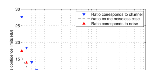
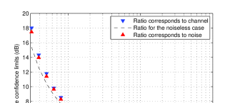
Figure 3: Ratios of the upper/lower confidence limits with SNR $=$ 10dB (left) and SNR $=$ 20dB (right)

For estimation of the SNR, there holds $\Pr\{D_{1}<\frac{\sigma_{H}^{2}}{\sigma_{V}^{2}}<D_{2}\}$ in light of Corollary 2 with

$$\frac{D_{2}}{D_{1}}=\frac{(1+\varepsilon)\overline{X_{1,N}^{2}}-(1-\varepsilon)\overline{X_{2,N}^{2}}}{(1-\varepsilon)\overline{X_{1,N}^{2}}-(1+\varepsilon)\overline{X_{2,N}^{2}}}$$

In Figure 4, the above is plotted against the sample size $N$ for the cases SNR = 10 and SNR $=$ 60.

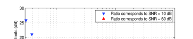
Figure 4: Ratios of the upper/lower confidence limits corresponds with $\delta=0.01$

It is commented that for both Figure 3 and Figure 4, the a priori bound $N>\frac{2(3+2\varepsilon)\ln(\frac{4}{\delta})}{3\varepsilon^{2}}$, rather than the relation in (28), is used. The results are nevertheless close to each other. In Figure 5, we plotted $\varepsilon$ vs. $N$ (left) for the case $\delta=0.05$, and plotted $\delta$ vs. $N$ (right) for the $\varepsilon=0.05$. In both cases, a priori bounds are used in both the noisy and noiseless cases, plus the use of $\chi^{2}$ in the noiseless case that is governed by the relation in (17).

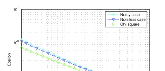
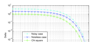
Figure 5: Plots of $\varepsilon$ vs. $N$ with $\delta=0.05$ (left), and $\delta$ vs. $N$ with $\varepsilon=0.05$ (right)

As expected, the curve based on $\chi^{2}$ CDF in the noiseless case serves as a lower bound. In addition it is observed that the two curves based on the a priori bounds are almost identical for the one on left, and close to each other for the one on right. This fact indicates that our results on measurement and estimation of noisy Rayleigh fading channels are not conservative. It is further observed that the $\varepsilon$ curves decrease at a constant slope in log-log scale, and the slope of decrease is rather slow with respect to the sample size $N$. This fact indicates that the reduction of $\varepsilon$ (with fixed $\delta$) is expensive in terms of increasing $N$. On the other hand the $\delta$ curves decrease at accelerated slopes with respect to the sample size $N$, implying that the reduction of $\delta$ (with fixed $\varepsilon$) is relatively cheap, especially at large sample size $N$. Figure 5 validates that the measurement sample size is roughly inversely proportional to the square of the margin of error $\varepsilon$ and is linear with respect to the logarithm of the inverse of the gap $\delta$.

The last simulation example is worked out to demonstrate the optimum estimator obtained in Theorem 5. Different from the previous two cases, $M(>>1)$ sets of measurement samples are taken to assess the average performance for the underlying statistical estimation. For each sample size $N$, $\{X_{\ell,i}(k)\}_{i=1}^{N}$ is generated for $\ell=1,2$, and $1\leq k\leq M$ with $M=500$. The optimum estimator in (36) is used to compute estimates $\widehat{\sigma}_{H,N}^{2}(k)$ and $\widehat{\sigma}_{V,N}^{2}(k)$. The estimation error is then averaged to yield

$${\rm RMES}_{H}\approx\sqrt{\frac{1}{M}\sum_{k=1}^{M}\left|\widehat{\sigma}_{H,N}^{2}(k)-\sigma_{H}^{2}\right|^{2}},\;\;\;\;\;{\rm RMES}_{V}\approx\sqrt{\frac{1}{M}\sum_{k=1}^{M}\left|\widehat{\sigma}_{V,N}^{2}(k)-\sigma_{V}^{2}\right|^{2}}$$

that are plotted together with the Cramér-Rao lower bounds:

$${\rm CRB}_{H}=\sqrt{\frac{(P_{s1}\sigma_{H}^{2}+\sigma_{V}^{2})^{2}+(P_{s2}\sigma_{H}^{2}+\sigma_{V}^{2})^{2}}{N\Delta P_{s}}},\;\;\;\;\;{\rm CRB}_{V}=\sqrt{\frac{P_{s2}^{2}(P_{s1}\sigma_{H}^{2}+\sigma_{V}^{2})^{2}+P_{s1}^{2}(P_{s2}\sigma_{H}^{2}+\sigma_{V}^{2})^{2}}{N\Delta P_{s}}}$$

versus the sample size $N$ as shown in Figure 6 where $P_{s2}=0$ is used. It can be seen that the RMSEs coincide very well with the CRBs, validating the optimality of the estimator in (36). Again the change of SNR affects little on estimation of $\sigma_{H}^{2}$ but changes the RMSE for $\sigma_{V}^{2}$ that is mainly due to the change of $\sigma_{V}^{2}$ by a factor of 10. In the case $M<500$, the RMSE lines are less straight and fluctuate more as $M$ becomes smaller, but the overall trend holds.

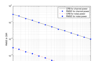
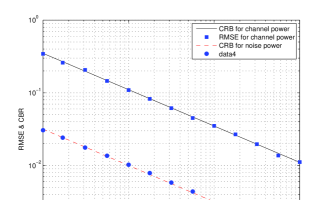
Figure 6: RMSE and CRB vs. $N$ with SNR $=$ 20dB (left) and SNR $=$ 10dB (right)

6 Conclusion

Statistical estimation of Rayleigh fading channels has been investigated based on both noiseless and noisy measurement samples. Complete solutions are derived for the associated sample complexity problem and provided for the optimum estimator problem in measurement and estimation of Rayleigh fading channels. Specifically our a priori bounds on measurement sample sizes ensure the prescribed margin of error and confidence level and are contrast to the existing work reported in the literature. In dealing with the noisy measurement samples, our proposed novel signaling scheme with two different signal strengths is instrumental in extracting the statistical information on mean channel power, noise power, and SNR. Such a novel signaling scheme enables us to derive the sample complexity bounds for both interval and point estimates that are tight for the mean channel power and noise power albeit less tight for the SNR. More importantly it leads to the optimum estimator that is both an ML and MV estimator and that achieves the Cramér-Rao lower bound. The results presented in this paper constitute an independent statistical theory for measurement and estimation of Rayleigh fading channels. It should be emphasized that the sample complexity solution in the noiseless case is also instrumental without which the results for the case of noisy measurements are not possible. The numerical simulations illustrate that our proposed statistical theory is effective in statistical estimation of Rayleigh fading channels. Specifically the simulation examples indicate that our results based on the noisy measurement samples are close to that based on the noiseless measurement samples, and the signal power is not required to be high that can be compensated for by using large sample size. Currently we are investigating the Nakagami fading channel which in a special case reduces to the Rayleigh fading channel, and aim at extension of our results on the measurement sample size and optimum estimator. It is our objective to apply our results to other more general wireless fading channels and to broad applications of our proposed statistical theory.

References

- [1] A. Abdi and M. Kaveh, “Performance comparison of three different estimators for the Nakagami parameter using Monte Carlo simulation,” IEEE Commun. Lett., vol. 4, pp. 119-121, April 2000.
- [2] P.A. Bello, “Characterization of randomly time-variant linear channels,” IEEE Trans. Commun., vol. 11, pp. 360–393, Dec. 1963.
- [3] J. Beek, O. Edfors, M. Sandell, S. Wilson, and P. Börjesson, “On channel estimation in OFDM systems,” in Proceedings of IEEE VTC 95, Chicago, 1995.
- [4] M. Barbiloni, C. Carciofi, G. Falciasecca, M. Frallone, and P. Grazioso, “A measurement-based methodology for the determination of validity domains of prediction models in urban environments,” IEEE Trans. Veh. Technol., vol. 49, pp. 1508-1515, Sept. 2000.
- [5] H. Chernoff, “A measure of asymptotic efficiency for tests of a hypothesis based on the sum of observations,” Annals of Mathematical Statistics, vol. 23, no. 4, pp. 493-507, 1952.
- [6] J. Cheng and N.C. Beaulieu, “Generalized moment estimators for the Nakagami fading parameters,” IEEE Commun. Lett., vol. 6, pp. 144-146, April 2002.
- [7] Y. Chen and N.C. Beaulieu, “Estimators using noisy channel samples for fading distribution parameters,” IEEE Trans. Commun., vol. 53, no. 8, Aug. 2005, pp. 1274-1277.
- [8] N. Cotanis, “Estimating radio coverage for new mobile wireless services data collection and pre-processing,” ICT2001, Bucharest, Romania, June 2001.
- [9] N. Czink, G. Matz, D. Seethaler, and F. Hlawatsch, “Improved MMSE estimation of correlated MIMO channels using a structured correlation estimator,” Proc. IEEE SPAWC-2005, New York, June 2005, pp. 595-599.
- [10] F.A. Dietrich, T. Ivanov, and W. Utschick, “Estimation of channel and noise correlations for MIMO channel estimation,” Proc. of the Workshop on Smart Antennas, Germany, 2006.
- [11] A. Dogandzic and J. Jin, “Estimating statistical properties of MIMO fading channels,” IEEE Transactions on Signal Processing, vol. 53, pp. 3065-3080, Aug. 2005.
- [12] G. Gu, J. He, X. Gao, and M. Naraghi-Pour, “An analytic approach to modeling and estimation of OFDM channels,” in Proceedings of IEEE 2004 Global Communications Conference (Dallas, TX), Nov. 2004, and to appear in IEEE Trans. Veh. Technol., July 2007.
- [13] M. Peritsky, “Statistical estimation of mean signal strength in a Rayleighfading environment,” IEEE Trans. Commun., vol. 21, no. 11, Nov. 1973, pp. 1207-1213.
- [14] J.D. Parsons, The mobile Radio Propagation Channel, Pentech House, 1994.
- [15] J.G. Proakis, Digital Communications, McGraw-Hill, 2000.
- [16] T.S. Rappaport, Wireless Communications — Principles and Practice, Prentice-Hall, Upper Saddle River, NJ, 1999.
- [17] M.K. Simon and M.-S. Alouini, “Average bit-error probability performance for optimum diversity combining of noncoherent FSK over Rayleigh fading channels,” IEEE Trans. Commun., vol. 51, pp. 566-569, April 2003.
- [18] G.L. Stber, Principles of Mobile Communication, second edition, Kluwer Academic Publishers, Norwell, MA, 2002.
- [19] C. Tepedelenlioglu, A. Abdi, and G.B. Giannakis, “The Rician factor: Estimation and performance analysis,” IEEE Trans. Wireless Commun., vol. 2, pp. 799-810, July 2003.
- [20] R.V. Valenzuela, O. Landron, and D.L. Jacobs, “Estimating local mean signal strength of indoor multipath propagation,” IEEE Trans. Veh. Technol., vol. 46, no. 1, Feb. 1997, pp. 203-212.