Lifetime Difference in $B_{s}$ mixing: Standard Model and beyond

Abstract

We present a calculation of $1/m^{2}_{b}$ corrections to the lifetime differences of $B_{s}$ mesons $\Delta\Gamma_{B_{s}}$ in the heavy-quark expansion. We find that they are small to significantly affect $\Delta\Gamma_{B_{s}}$ and present the result for lifetime difference including non-perturbative $1/m_{b}$ and $1/m_{b}^{2}$ corrections. We also analyze the generic $\Delta B=1$ New Physics contributions to $\Delta\Gamma_{B_{s}}$ and provide several examples.

I Introduction

Meson-antimeson mixing serves as an indispensable way of placing constraints on various models of New Physics (NP). This is usually ascribed to the fact that this process only occurs at the one-loop level in the Standard Model (SM) of electroweak interactions. This makes it sensitive to the effects of possible NP particles in the loops or even to new tree-level interactions that can possibly contribute to the flavor-changing $\Delta Q=2$ interactions. These interactions induce non-diagonal terms in the meson-antimeson mass matrix that describes the dynamics of those states. Diagonalizing this mass matrix gives two mass eigenstates that are superpositions of flavor eigenstates. In the $B_{s}$ system mass eigenstates, denoted as “heavy” $|B_{H}\rangle$ and “light” $|B_{L}\rangle$,

$$|B_{H}\rangle = p|B_{s}\rangle+q|\overline{B}_{s}\rangle,$$

$$|B_{L}\rangle = p|B_{s}\rangle-q|\overline{B}_{s}\rangle,$$ (1)

were predicted to have a rather significant mass and width differences,

$$\Delta M_{B_{s}}=M_{H}-M_{L},\qquad\Delta\Gamma_{B_{s}}=\Gamma_{L}-\Gamma_{H},$$ (2)

where $M_{H,L}$ and $\Gamma_{H,L}$ denote mass and lifetime differences of mass eigenstates. Since in the Standard Model the mass difference is dominated by the top quark contributions, it is computable with great accuracy. Thus one might expect that possible NP contributions can be easily isolated. Unfortunately, a recent observation of mass difference of mass eigenstates in $B_{s}$ mixing by CDF Abulencia:2006ze and D0 Abazov:2006dm ,

$$\Delta M_{B_{s}}=17.77\pm 0.10\pm 0.07\mbox{~{}ps}^{-1}\mbox{~{}~{}(CDF)},$$

$$17\mbox{~{}ps}^{-1}<\Delta M_{B_{s}}<21\mbox{~{}ps}^{-1}\mbox{~{}~{}~{}~{}~{}(D0)},$$ (3)

put the hopes of spectacular NP effects in $B_{s}$ system rest. In fact, analyses of mixing in the strange, charm and beauty quark systems all yielded positive signals, yet all of those signals seem to be explained quite well by the SM interactions. Yet, some contribution from New Physics particles is still possible, so even the energy scales above those directly accessible at the Tevatron or LHC can be probed with $B_{s}$ mixing, provided that QCD sum rule Korner:2003zk or lattice QCD Dalgic:2006gp ; Becirevic:2001xt ; Gimenez:2000jj ; Aoki:2003xb calculations supply the relevant hadronic parameters with sufficient accuracy.

In addition to the mass difference $\Delta M_{B_{s}}$, a number of experimental collaborations reported the observation of a lifetime difference $\Delta\Gamma_{B_{s}}$ in the $B_{s}$ system. Combining recent result from D0 Abazov:2007tx with earlier measurements from CDF Acosta:2004gt and ALEPH Barate:2000kd , Particle Data Group (PDG) quotes PDG

$$\Delta\Gamma_{B_{s}}=0.16^{+0.10}_{-0.13}\mbox{~{}ps}^{-1},\qquad\frac{\Delta\Gamma_{B_{s}}}{\Gamma_{B_{s}}}=0.121^{+0.083}_{-0.090},$$ (4)

while Heavy Flavor Averaging Group (HFAG) Barberio:2007cr gives

$$\Delta\Gamma_{B_{s}}=0.071^{+0.053}_{-0.057}\mbox{~{}ps}^{-1},\qquad\frac{\Delta\Gamma_{B_{s}}}{\Gamma_{B_{s}}}=0.104^{+0.076}_{-0.084}.$$ (5)

Differently from the mass difference $\Delta M_{B_{s}}$, the lifetime difference $\Delta\Gamma_{B_{s}}$ is definitely dominated by the SM contributions, as it is generated by the on-shell intermediate states Beneke:1996gn ; Beneke:1998sy ; Ciuchini:2003ww ; Lenz:2006hd . While this might appear to make it less exciting for indirect searches for New Physics, besides “merely” providing yet another test for heavy quark expansion, it is nonetheless a useful quantity for a combined analysis of possible NP contributions to $B_{s}{}^{0}-\overline{B}_{s}{}^{0}$ mixing Grossman:2006ce ; Ligeti:2006pm ; Grossman:1996er ; Dunietz:2000cr .

It has been argued Grossman:1996er that CP-violating NP contributions to $\Delta B=2$ amplitudes can only reduce the experimentally-observed lifetime difference compared to its SM value, therefore it is important to have an accurate theoretical evaluation of $\Delta\Gamma_{B_{s}}$ in the SM. It is also important to note that $\Delta B=1$ NP contributions can affect $\Delta\Gamma_{B_{s}}$, but do not have to follow the same pattern. Indeed, the level at which $\Delta B=1$ NP can affect $\Delta\Gamma_{B_{s}}$ depends both on the particular extension of the SM, as well as on the projected accuracy of lattice calculations of hadronic parameters which drives the uncertainties on the theoretical prediction of $\Delta\Gamma_{B_{s}}$. So it is advantageous to evaluate the effect of NP contributions.

This paper is organized as follows. We set up the relevant formalism and argue for the need to compute $1/m^{2}_{b}$ corrections to leading and next-to-leading effects in Sect. II. In Sect. III we discuss the impact of $1/m^{2}_{b}$ corrections to the lifetime differences of $B_{s}$ mesons and assess the convergence of the $1/m_{b}$ expansion. We also present the complete SM results for $\Delta\Gamma_{B_{s}}$ including $1/m_{b}^{2}$ corrections. We then discuss the possible effects from $\Delta B=1$ New Physics contributions in Sect. IV. Finally, we present our conclusions in Sect. V.

II Formalism

In the limit of exact CP conservation the mass eigenstates of the $B_{s}^{0}$–$\overline{B}^{0}_{s}$ system are $|B_{H/L}\rangle=(|B_{s}\rangle\pm|\overline{B}_{s}\rangle)/\sqrt{2}$, with the convention $CP|B_{s}\rangle=-|\overline{B}_{s}\rangle$. The width difference between mass eigenstates is then given by Beneke:1996gn

$$\Delta\Gamma_{B_{s}}\equiv\Gamma_{L}-\Gamma_{H}=-2\,\Gamma_{12}=-2\,\Gamma_{21},$$ (6)

where $\Gamma_{ij}$ are the elements of the decay-width matrix, $i,j=1,2$ ($|1\rangle=|B_{s}\rangle$, $|2\rangle=|\overline{B}_{s}\rangle$).

We use the optical theorem to relate the off-diagonal elements of the decay-width matrix $\Gamma$ entering the neutral $B$-meson oscillations to the imaginary part of the forward matrix element of the transition operator ${\cal T}$:

$$\Gamma_{21}(B_{s})=\frac{1}{2M_{B_{s}}}\langle\overline{B}_{s}|{\cal T}|B_{s}\rangle,\quad{\cal T}={\mbox{Im}}~{}i\int d^{4}xT\left\{H_{\mbox{\scriptsize eff}}(x)H_{\mbox{\scriptsize eff}}(0)\right\}.$$ (7)

Here ${\cal H}_{eff}$ is the low energy effective weak Hamiltonian mediating bottom-quark decays. The component that is relevant for $\Gamma_{21}$ reads explicitly

$${\cal H}_{eff}=\frac{G_{F}}{\sqrt{2}}V^{*}_{cb}V^{\phantom{*}}_{cs}\left(\,\sum^{6}_{r=1}C_{r}Q_{r}+C_{8}Q_{8}\right),$$ (8)

defining the operators

$$Q_{1}=(\bar{b}_{i}c_{j})_{V-A}(\bar{c}_{j}s_{i})_{V-A},\qquad Q_{2}=(\bar{b}_{i}c_{i})_{V-A}(\bar{c}_{j}s_{j})_{V-A},$$ (9)

$$Q_{3}=(\bar{b}_{i}s_{i})_{V-A}(\bar{q}_{j}q_{j})_{V-A},\qquad Q_{4}=(\bar{b}_{i}s_{j})_{V-A}(\bar{q}_{j}q_{i})_{V-A},$$ (10)

$$Q_{5}=(\bar{b}_{i}s_{i})_{V-A}(\bar{q}_{j}q_{j})_{V+A},\qquad Q_{6}=(\bar{b}_{i}s_{j})_{V-A}(\bar{q}_{j}q_{i})_{V+A},$$ (11)

$$Q_{8}=\frac{g}{8\pi^{2}}m_{b}\,\bar{b}_{i}\sigma^{\mu\nu}(1-\gamma_{5})T^{a}_{ij}s_{j}\,G^{a}_{\mu\nu}.$$ (12)

Here $i,j$ are color indices and a summation over $q=u$, $d$, $s$, $c$, $b$ is implied. $V\pm A$ refers to $\gamma^{\mu}(1\pm\gamma_{5})$ and $S-P$ (which we need below) to $(1-\gamma_{5})$. $C_{1},\ldots,C_{6}$ are the corresponding Wilson coefficient functions at the renormalization scale $\mu$, which are known at next-to-leading order. We have also included the chromomagnetic operator $Q_{8}$, contributing to ${\cal T}$ at ${\cal O}(\alpha_{s})$. Note that for a negative $C_{8}$, as conventionally used in the literature, the Feynman rule for the quark-gluon vertex is $-ig\gamma_{\mu}T^{a}$. A detailed review and explicit expressions may be found in Buchalla:1995vs . Cabibbo-suppressed channels have been neglected in Eq. (8).

In the heavy-quark limit, the energy release supplied by the b-quark is large, so the correlator in Eq. (7) is dominated by short-distance physics Shifman:1984wx . An Operator Product Expansion (OPE) can be constructed for Eq. (7), which results in its expansion as a series of matrix elements of local operators of increasing dimension suppressed by powers of $1/m_{b}$:

$$\Gamma_{21}(B_{s})=\frac{1}{2M_{B_{s}}}\sum_{k}\langle B_{s}|{\cal T}_{k}|B_{s}\rangle=\sum_{k}\frac{C_{k}(\mu)}{m_{b}^{k}}\langle B_{s}|{\cal O}_{k}^{\Delta B=2}(\mu)|B_{s}\rangle.$$ (13)

In other words, the calculation of $\Gamma_{21}(B_{s})$ is equivalent to computing the matching coefficients of the effective $\Delta B=2$ Lagrangian with subsequent computation of its matrix elements. Eventually the scale dependence of the Wilson coefficients in Eq. (13) is bound to match the scale dependence of the computed matrix elements.

Expanding the operator product (7) for small $x\sim 1/m_{b}$, the transition operator ${\cal T}$ can be written to leading order in the $1/m_{b}$ expansion as Beneke:1996gn ; Beneke:1998sy

$${\cal T}=-\frac{G^{2}_{F}m^{2}_{b}}{12\pi}(V^{*}_{cb}V^{\phantom{*}}_{cs})^{2}\,\left[F(z)Q(\mu_{2})+F_{S}(z)Q_{S}(\mu_{2})\right],$$ (14)

which results in Ciuchini:2003ww

$$\Gamma {}_{21}(B_{s})=-\frac{G^{2}_{F}m^{2}_{b}}{12\pi(2M_{B_{s}})}(V^{*}_{cb}V^{\phantom{*}}_{cs})^{2}\sqrt{1-4z}\times$$ (15)

$$\times \left\{\left[(1-z)\,\left(2\,C_{1}C_{2}+N_{c}C^{2}_{2}\right)+(1-4z)C^{2}_{1}/2\right]\langle Q\rangle+(1+2z)\left(2\,C_{1}C_{2}+N_{c}C^{2}_{2}-C^{2}_{1}\right)\langle Q_{S}\rangle\right\},$$

with $z=m_{c}^{2}/m_{b}^{2}$ and the basis of $\Delta B=2$ operators

$$Q=(\bar{b}_{i}s_{i})_{V-A}(\bar{b}_{j}s_{j})_{V-A},\qquad Q_{S}=(\bar{b}_{i}s_{i})_{S-P}(\bar{b}_{j}s_{j})_{S-P}~{}.$$ (16)

In writing Eq. (14) we have used the Fierz identities and the equations of motion to eliminate the color re-arranged operators

$$\tilde{Q}=(\bar{b}_{i}s_{j})_{V-A}(\bar{b}_{j}s_{i})_{V-A},\qquad\tilde{Q}_{S}=(\bar{b}_{i}s_{j})_{S-P}(\bar{b}_{j}s_{i})_{S-P}~{},$$ (17)

always working to leading order in $1/m_{b}$. Note that $\langle...\rangle$ denote matrix elements of the above operators taken between $B_{s}$ and ${\overline{B}}_{s}$ states. The Wilson coefficients $F$ and $F_{S}$ can be extracted by computing the matrix elements between quark states of ${\cal T}$ in Eq. (7).

The coefficients in the transition operator (14) at next-to-leading order, still neglecting the penguin sector, can be written as Beneke:1998sy :

$$F(z)=F_{11}(z)C^{2}_{2}(\mu_{1})+F_{12}(z)C_{1}(\mu_{1})C_{2}(\mu_{1})+F_{22}(z)C^{2}_{1}(\mu_{1}),$$ (18)

$$F_{ij}(z)=F^{(0)}_{ij}(z)+\frac{\alpha_{s}(\mu_{1})}{4\pi}F^{(1)}_{ij}(z),$$ (19)

and similarly for $F_{S}(z)$. The leading order functions $F^{(0)}_{ij}$, $F^{(0)}_{S,ij}$ read explicitly

$$F^{(0)}_{11}(z)=3\sqrt{1-4z}\,(1-z),\qquad F^{(0)}_{S,11}(z)=3\sqrt{1-4z}\,(1+2z),$$ (20)

$$F^{(0)}_{12}(z)=2\sqrt{1-4z}\,(1-z),\qquad F^{(0)}_{S,12}(z)=2\sqrt{1-4z}\,(1+2z),$$ (21)

$$\,F^{(0)}_{22}(z)=\frac{1}{2}(1-4z)^{3/2},\qquad\qquad F^{(0)}_{S,22}(z)=-\sqrt{1-4z}\,(1+2z).$$ (22)

The next-to-leading order (NLO) expressions $F^{(1)}_{ij}$, $F^{(1)}_{S,ij}$ are given in Ref. Beneke:1998sy .

The penguin correction to Eq. (14),

$${\cal T}_{p}=-\frac{G^{2}_{F}m^{2}_{b}}{12\pi}(V^{*}_{cb}V^{\phantom{*}}_{cs})^{2}\,\left[P(z)Q+P_{S}(z)Q_{S}\right],$$ (23)

is also shown in Ref. Beneke:1998sy .

III Subleading $1/m_{b}^{n}$ corrections

Here we present the higher order corrections to $\Gamma_{21}(B_{s})$ in Eq. (15) in the heavy-quark expansion, denoted below as $\delta_{1/m}$ and $\delta_{1/m^{2}}$:

$$\Gamma_{21}(B_{s})=-\frac{G^{2}_{F}m^{2}_{b}}{12\pi(2M_{B_{s}})}(V^{*}_{cb}V^{\phantom{*}}_{cs})^{2}\,\left\{\left[F(z)+P(z)\right]\langle Q\rangle+\left[F_{S}(z)+P_{S}(z)\right]\langle Q_{S}\rangle+\delta_{1/m}+\delta_{1/m^{2}}\right\}\,.$$ (24)

The matrix elements for $Q$ and $Q_{S}$ are known to be Beneke:1996gn ; Beneke:1998sy ; Ciuchini:2003ww

$$\langle Q\rangle \equiv \langle\overline{B}_{s}|Q|B_{s}\rangle=f^{2}_{B_{s}}M^{2}_{B_{s}}2\left(1+\frac{1}{N_{c}}\right)B,$$

$$\langle Q_{S}\rangle \equiv \langle\overline{B}_{s}|Q_{S}|B_{s}\rangle=-f^{2}_{B_{s}}M^{2}_{B_{s}}\frac{M^{2}_{B_{s}}}{(m_{b}+m_{s})^{2}}\left(2-\frac{1}{N_{c}}\right)B_{S},$$ (25)

$$\delta_{1/m} = \langle\overline{B}_{s}|{\cal T}_{1/m}|B_{s}\rangle,\qquad\mbox{and}\qquad\delta_{1/m^{2}}=\langle\overline{B}_{s}|{\cal T}_{1/m^{2}}|B_{s}\rangle,$$

where $M_{B_{s}}$ and $f_{B_{s}}$ are the mass and decay constant of the $B_{s}$ meson and $N_{c}$ is the number of colors. The parameters $B$ and $B_{S}$ are defined such that $B=B_{S}=1$ corresponds to the factorization (or ‘vacuum insertion’) approach, which can provide a first estimate.

III.1 $1/m_{b}$ corrections

Figure 1: Calculation of kinetic $1/m_{b}$ and $1/m_{b}^{2}$ corrections. The operators of Eqs. (26) and (30) are obtained by expanding the diagrams in powers of light quark momentum.

The $1/m_{b}$ corrections are computed, as in Ref. Beneke:1996gn ; Ciuchini:2003ww ; Shifman:1984wx ; Gabbiani:2004tp , by expanding the forward scattering amplitude of Eq. (7) in the light-quark momentum and matching the result onto the operators containing derivative insertions (see Fig. 1). The $\delta_{1/m}$ contributions can be written in the following form:

$${\cal T}_{1/m} = \sqrt{1-4z}\left\{(1+2z)\left[C^{2}_{1}\,\left(R_{2}+2R_{4}\right)-2\,(2\,C_{1}C_{2}+N_{c}C_{2}^{2})\,\left(R_{1}+R_{2}\right)\right]\phantom{\frac{z^{2}}{4}}\right.$$ (26)

$$- \left.\frac{12z^{2}}{1-4z}\left[(2\,C_{1}C_{2}+N_{c}C^{2})\,\left(R_{2}+2R_{3}\right)+2\,C^{2}_{1}\,R_{3}\right]\right\},$$

where the operators $R_{i}$ are defined as

$$R_{1} = {\displaystyle{m_{s}\over m_{b}}}\bar{b}_{i}\gamma^{\mu}(1-\gamma_{5})s_{i}~{}\bar{b}_{j}\gamma_{\mu}(1+\gamma_{5})s_{j}\,,\qquad\ \ R_{2}={\displaystyle{1\over m^{2}_{b}}}\bar{b}_{i}{\overleftarrow{D}}_{\!\rho}\gamma^{\mu}(1-\gamma_{5})\overrightarrow{D}^{\rho}s_{i}~{}\bar{b}_{j}\gamma_{\mu}(1-\gamma_{5})s_{j}\,,$$

$$R_{3} = {\displaystyle{1\over m^{2}_{b}}}\bar{b}_{i}{\overleftarrow{D}}_{\!\rho}(1-\gamma_{5})\overrightarrow{D}^{\rho}s_{i}~{}\bar{b}_{j}(1-\gamma_{5})s_{j}\,,\qquad R_{4}={\displaystyle{1\over m_{b}}}\bar{b}_{i}(1-\gamma_{5})i\overrightarrow{D}_{\mu}s_{i}~{}\bar{b}_{j}\gamma^{\mu}(1-\gamma_{5})s_{j}\,.$$ (27)

Their matrix elements read Beneke:1996gn ; Ciuchini:2003ww :

$$\langle\overline{B}_{s}|R_{1}|B_{s}\rangle = \left(2+\frac{1}{N_{c}}\right)\,{\displaystyle{m_{s}\over m_{b}}}\,f_{B_{s}}^{2}M_{B_{s}}^{2}\,B^{s}_{1},\quad\quad\langle\overline{B}_{s}|R_{2}|B_{s}\rangle=\left(-1+\frac{1}{N_{c}}\right)\,f_{B_{s}}^{2}M_{B_{s}}^{2}\left({\displaystyle{M_{B_{s}}^{2}\over m_{b}^{2}}}-1\right)\,B^{s}_{2},$$

$$\langle\overline{B}_{s}|R_{3}|B_{s}\rangle = \left(1+\frac{1}{2N_{c}}\right)\,f_{B_{s}}^{2}M_{B_{s}}^{2}\left({\displaystyle{M_{B_{s}}^{2}\over m_{b}^{2}}}-1\right)\,B^{s}_{3},\quad\langle\overline{B}_{s}|R_{4}|B_{s}\rangle=-f_{B_{s}}^{2}M_{B_{s}}^{2}\left({\displaystyle{M_{B_{s}}^{2}\over m_{b}^{2}}}-1\right)\,B^{s}_{4}\,.$$ (28)

Some of those parameters have been computed in lattice QCD Dalgic:2006gp ; Becirevic:2001xt ; Gimenez:2000jj ; Aoki:2003xb . In this paper we use the results of Ref. Dalgic:2006gp .

The color-rearranged operators $\widetilde{R}_{i}$ that follow from the expressions for $R_{i}$ by interchanging color indexes of $b_{i}$ and $s_{j}$ Dirac spinors have been eliminated using Fierz identities and the equations of motion as in Eq. (16). Note that the above result contains full QCD $b$-fields, thus there is no immediate power counting available for these operators. The power counting becomes manifest at the level of the matrix elements.

III.2 $1/m^{2}_{b}$ corrections

It was shown in Refs. Beneke:1996gn ; Ciuchini:2003ww that $1/m_{b}$-corrections are quite large, so it is important to assess the convergence of $1/m_{b}$-expansion in the calculation of the $B_{s}$ lifetime difference. In order to do so, we compute a set of $\delta_{1/m_{b}^{2}}$ corrections to leading order. As expected, at this order more operators will contribute. We will parametrize the $1/m_{b}^{2}$ corrections similarly to our parametrization of $1/m_{b}$ effects above and use the factorization approximation to assess their contributions to the $B_{s}$ lifetime difference.

Figure 2: $1/m_{b}^{2}$-corrections from gluonic operators.

Two classes of corrections arise at this order. One class involves kinetic corrections which can be computed in a way analogous to the previous case by expanding the forward scattering amplitudes in the powers of the light-quark momentum. A second class involves corrections arising from the interaction with background gluon fields. The complete set of corrections is the sum of those,

$${\cal T}_{1/m^{2}}={\cal T}_{1/m^{2}}^{kin}+{\cal T}_{1/m^{2}}^{G}.$$ (29)

Let us consider those classes of corrections in turn. The kinetic corrections can be written as

$${\cal T}_{1/m^{2}}^{kin} = \sqrt{1-4z}\Bigl{[}{\displaystyle{24z^{2}\over(1-4z)^{2}}}(3-10z)\left[C_{1}^{2}W_{3}+(2\,C_{1}C_{2}+N_{c}C_{2}^{2})(W_{3}+W_{2}/2)\right]$$ (30)

$$+ {\displaystyle{12z^{2}\over 1-4z}}{\displaystyle{m_{s}^{2}\over m_{b}^{2}}}\left[C_{1}^{2}Q_{S}-(2\,C_{1}C_{2}+N_{c}C_{2}^{2})(Q_{S}+Q/2)\right]$$

$$+ {\displaystyle{24z^{2}\over 1-4z}}\left[2C_{1}^{2}W_{4}-2\,(2\,C_{1}C_{2}+N_{c}C_{2}^{2})(W_{1}+W_{2}/2)\right]$$

$$- (1-2z){\displaystyle{m_{s}^{2}\over m_{b}^{2}}}(C_{1}^{2}+2\,C_{1}C_{2}+N_{c}C_{2}^{2})Q_{R}\Bigr{]}.$$

We again retain the dependence on quark masses in the above expression, including the terms proportional to $m_{s}$. The operators in Eq. (30) are defined as

$$Q_{R} = (\bar{b}_{i}s_{i})_{S+P}(\bar{b}_{j}s_{j})_{S+P}\,,$$

$$W_{1} = {\displaystyle{m_{s}\over m_{b}}}\bar{b}_{i}\overleftarrow{D}^{\alpha}(1-\gamma_{5})\overrightarrow{D}_{\alpha}s_{i}~{}\bar{b}_{j}(1+\gamma_{5})s_{j}\,,$$

$$W_{2} = {\displaystyle{1\over m_{b}^{4}}}\bar{b}_{i}\overleftarrow{D}^{\alpha}\overleftarrow{D}^{\beta}\gamma^{\mu}(1-\gamma_{5})\overrightarrow{D}_{\alpha}\overrightarrow{D}_{\beta}s_{i}~{}\bar{b}_{j}\gamma_{\mu}(1-\gamma_{5})s_{j}\,,$$

$$W_{3} = {\displaystyle{1\over m_{b}^{4}}}\bar{b}_{i}\overleftarrow{D}^{\alpha}\overleftarrow{D}^{\beta}(1-\gamma_{5})\overrightarrow{D}_{\alpha}\overrightarrow{D}_{\beta}s_{i}~{}\bar{b}_{j}(1-\gamma_{5})s_{j}\,,$$

$$W_{4} = {\displaystyle{1\over m_{b}^{4}}}\bar{b}_{i}\overleftarrow{D}^{\alpha}(1-\gamma_{5})i\overrightarrow{D}_{\mu}\overrightarrow{D}_{\alpha}s_{i}~{}\bar{b}_{j}\gamma^{\mu}(1-\gamma_{5})s_{j}\,,$$ (31)

where, as before, we have eliminated the color-rearranged operators $\widetilde{W}_{i}$ in favor of the operators $W_{i}$. The parametrization of the matrix elements of the above operators is given below,

$$\langle\overline{B}_{s}|Q_{R}|B_{s}\rangle = -\left(2-\frac{1}{N_{c}}\right)f^{2}_{B_{s}}M^{2}_{B_{s}}\frac{M^{2}_{B_{s}}}{(m_{b}+m_{s})^{2}}\alpha_{1}\,,$$

$$\langle\overline{B}_{s}|W_{1}|B_{s}\rangle = {\displaystyle{m_{s}\over m_{b}}}\left(1+\frac{1}{2N_{c}}\right)\,f_{B_{s}}^{2}M_{B_{s}}^{2}\left({\displaystyle{M_{B_{s}}^{2}\over m_{b}^{2}}}-1\right)\alpha_{2}\,,$$

$$\langle\overline{B}_{s}|W_{2}|B_{s}\rangle = \frac{1}{2}\left(-1+\frac{1}{N_{c}}\right)\,f_{B_{s}}^{2}M_{B_{s}}^{2}\left({\displaystyle{M_{B_{s}}^{2}\over m_{b}^{2}}}-1\right)^{2}\alpha_{3}\,,$$

$$\langle\overline{B}_{s}|W_{3}|B_{s}\rangle = \frac{1}{2}\left(1+\frac{1}{2N_{c}}\right)\,f_{B_{s}}^{2}M_{B_{s}}^{2}\left({\displaystyle{M_{B_{s}}^{2}\over m_{b}^{2}}}-1\right)^{2}\alpha_{4}\,,$$

$$\langle\overline{B}_{s}|W_{4}|B_{s}\rangle = -\frac{1}{2}\,f_{B_{s}}^{2}M_{B_{s}}^{2}\left({\displaystyle{M_{B_{s}}^{2}\over m_{b}^{2}}}-1\right)^{2}\alpha_{5}\,.$$ (32)

Note that in factorization approximation all the bag parameters $\alpha_{i}$ should be set to 1. In addition to the set of kinetic corrections considered above, the effects of the interactions of the intermediate quarks with background gluon fields should also be included at this order. The contribution of those operators can be computed from the diagram of Fig. 2, resulting in

$${\cal T}_{1/m^{2}}^{G}= - {\displaystyle{G_{F}^{2}(V^{*}_{cb}V^{\phantom{*}}_{cs})^{2}\over 4\pi\sqrt{1-4z}}}\left\{C_{1}^{2}\left[(1-4z)P_{1}-(1-4z)P_{2}+4zP_{3}-4zP_{4}\right]\right.$$ (33)

$$+ \left.4\;C_{1}C_{2}z\left[P_{5}+P_{6}-P_{7}-P_{8}\right]\phantom{C^{2}_{1}}\hskip-15.0pt\right\}.$$

The local four-quark operators in the above formulas are shown in Eq. (III.2):

$$P_{1} = \bar{b}_{i}\gamma^{\mu}(1-\gamma_{5})s^{\phantom{l}}_{i}~{}\bar{b}^{\phantom{l}}_{k}\gamma^{\nu}(1-\gamma_{5})t_{kl}^{a}\widetilde{G}_{\mu\nu}^{a}s^{\phantom{l}}_{l}\,,$$

$$P_{2} = \bar{b}_{k}\gamma^{\mu}(1-\gamma_{5})t_{kl}^{a}\widetilde{G}_{\mu\nu}^{a}s_{l}~{}\bar{b}^{\phantom{l}}_{i}\gamma^{\nu}(1-\gamma_{5})s^{\phantom{l}}_{i}\,,$$

$$P_{3} = {\displaystyle{1\over m_{b}^{2}}}\bar{b}_{i}\overleftarrow{D}^{\mu}\overleftarrow{D}^{\alpha}\gamma^{\alpha}(1-\gamma_{5})s^{\phantom{l}}_{i}~{}\bar{b}^{\phantom{l}}_{k}\gamma_{\nu}(1-\gamma_{5})t_{kl}^{a}\widetilde{G}_{\mu\nu}^{a}s^{\phantom{l}}_{l}\,,$$

$$P_{4} = {\displaystyle{1\over m_{b}^{2}}}\bar{b}_{k}\overleftarrow{D}^{\nu}\overleftarrow{D}^{\alpha}\gamma^{\mu}(1-\gamma_{5})t_{kl}^{a}\widetilde{G}_{\mu\nu}^{a}s^{\phantom{l}}_{l}~{}\bar{b}^{\phantom{l}}_{i}\gamma_{\alpha}(1-\gamma_{5})s^{\phantom{l}}_{i}\,,$$

$$P_{5} = {\displaystyle{1\over m_{b}^{2}}}\bar{b}_{k}\overleftarrow{D}^{\nu}\overleftarrow{D}^{\alpha}\gamma^{\mu}(1-\gamma_{5})s^{\phantom{l}}_{i}~{}t_{kl}^{a}\widetilde{G}_{\mu\nu}^{a}~{}\bar{b}^{\phantom{l}}_{i}\gamma_{\alpha}(1-\gamma_{5})s^{\phantom{l}}_{l}\,,$$

$$P_{6} = {\displaystyle{1\over m_{b}^{2}}}\bar{b}_{i}\overleftarrow{D}^{\nu}\overleftarrow{D}^{\alpha}\gamma^{\mu}(1-\gamma_{5})s^{\phantom{l}}_{k}~{}t_{kl}^{a}\widetilde{G}_{\mu\nu}^{a}~{}\bar{b}^{\phantom{l}}_{l}\gamma_{\alpha}(1-\gamma_{5})s^{\phantom{l}}_{i}\,,$$

$$P_{7} = {\displaystyle{1\over m_{b}^{2}}}\bar{b}_{k}\overleftarrow{D}^{\mu}\overleftarrow{D}^{\alpha}\gamma^{\alpha}(1-\gamma_{5})s^{\phantom{l}}_{i}~{}t_{kl}^{a}\widetilde{G}_{\mu\nu}^{a}~{}\bar{b}^{\phantom{l}}_{i}\gamma_{\nu}(1-\gamma_{5})s^{\phantom{l}}_{l}\,,$$

$$P_{8} = {\displaystyle{1\over m_{b}^{2}}}\bar{b}_{i}\overleftarrow{D}^{\mu}\overleftarrow{D}^{\alpha}\gamma^{\alpha}(1-\gamma_{5})s^{\phantom{l}}_{k}~{}t_{kl}^{a}\widetilde{G}_{\mu\nu}^{a}~{}\bar{b}^{\phantom{l}}_{l}\gamma_{\nu}(1-\gamma_{5})s^{\phantom{l}}_{i}.$$ (34)

Analogously to the previous section, and following Ref. Gabbiani:2004tp , we parametrize the matrix elements in Eq. (III.2) as

$$\langle\overline{B}_{s}|P_{i}|B_{s}\rangle={\displaystyle{1\over 4}}f^{2}_{B_{s}}M^{2}_{B_{s}}\left({\displaystyle{M_{B_{s}}^{2}\over m^{2}_{b}}}-1\right)^{2}\beta_{i}.$$ (35)

We set $\beta_{i}$ = 1$~{}GeV^{2}$ to obtain a numerical estimate of this effect. It is clear that no precise prediction is possible with so many operators contributing to the lifetime difference. This, of course, is expected, as the number of contributing operators always increases significantly with each order in OPE. We can nonetheless evaluate the contribution of both $1/m_{b}$ and $1/m_{b}^{2}$ by randomly varying the parameters describing the matrix elements by $\pm 30\%$ around their “factorized” values. This way we obtain the interval of predictions of $\Delta\Gamma_{B_{s}}$ and estimate the uncertainty of our result.

III.3 Discussion

Now we discuss the phenomenological implications of the results presented in the previous sections. As usual in OPE-based calculations next-order corrections bring new unknown coefficients. In our numerical results we assume the value of the $b$-quark pole mass to be $m_{b}=4.8\pm 0.2$ GeV and $f_{B_{s}}$ = 230 $\pm$ 25 MeV. It might be advantageous to see what effects higher-order $1/m_{b}^{2}$ corrections have on the value of $\Delta\Gamma_{B_{s}}$. In order to see that we fix all perturbative parameters at the middle of their allowed ranges and show the dependence of $\Delta\Gamma_{B_{s}}$ on non-perturbative parameters defined in Eqs. (III.1), (III.2), and (35):

$$\Delta\Gamma_{B_{s}}\ = \ \Bigl{[}0.0005B+0.1732B_{s}+0.0024B_{1}-0.0237B_{2}-0.0024B_{3}-0.0436B_{4}$$

$$+ \ 2\times 10^{-5}\alpha_{1}+4\times 10^{-5}\alpha_{2}+4\times 10^{-5}\alpha_{3}+0.0009\alpha_{4}-0.0007\alpha_{5}$$

$$+ \ 0.0002\beta_{1}-0.0002\beta_{2}+6\times 10^{-5}\beta_{3}-6\times 10^{-5}\beta_{4}-1\times 10^{-5}\beta_{5}$$

$$- \ 1\times 10^{-5}\beta_{6}+1\times 10^{-5}\beta_{7}+1\times 10^{-5}\beta_{8}\Bigr{]}\quad(\mbox{ps}^{-1}).$$

As one can see, $1/m_{b}^{2}$ corrections provide rather minor overall impact on the calculation of $\Delta\Gamma_{B_{s}}$. In particular, contributions of gluonic operators are essentially negligible.

To obtain the complete Standard Model estimate of $\Delta\Gamma_{B_{s}}$, we fix the perturbative scale in our calculations to $\mu=m_{b}$ and vary the values of parameters of the matrix elements. Following Gabbiani:2004tp we adopt the statistical approach for presenting our results and generate 100000-point probability distributions of the lifetime, obtained by randomly varying our parameters within a $\pm 30\%$ interval around their “factorization” values. The decay constant $f_{B_{s}}$ and the b-quark pole mass $m_{b}$ are taken to vary within a $1\sigma$ interval as indicated above. The results are presented in Fig. 3. This figure represents the main result of this paper ICHEP2006 .

Figure 3: Histogram showing the random distribution around the central values of various parameters of Eqs. (24, 26, 30, 33) contributing to $B_{s}$-lifetime difference $\Delta\Gamma_{B_{s}}$.

There is no theoretically-consistent way to translate the histogram of Figure 3 into numerical predictions for $\Delta\Gamma_{B_{s}}$. As a useful estimate we give a numerical prediction by estimating the width of the distribution Fig. 3 at the middle of its height and position of the maximum of the curve as the most probable value. We caution that predictions obtained this way should be treated with care, as it is not expected that the theoretical predictions are distributed according to the Gaussian distribution. Nevertheless, following the procedure described above one obtains

$$\Delta\Gamma_{B_{s}}=0.072^{+0.034}_{-0.030}~{}\mbox{ps}^{-1},\quad\frac{\Delta\Gamma_{B_{s}}}{\Gamma_{B_{s}}}=0.104\pm 0.049,$$ (37)

where we added the experimental error from the determination of $\Gamma_{s}$ and theoretical error from our calculation of $\Delta\Gamma_{B_{s}}$ in quadrature.

IV New Physics contributions to lifetime difference

In the previous section we have shown that $1/m_{b}^{2}$-corrections to the lifetime difference of the light and heavy eigenstates in the $B_{s}$ system are quite small, which makes the prediction of $\Delta\Gamma_{B_{s}}$ quite reliable . Additionally improving the accuracy of the lattice or QCD sum rule determinations of non-perturbative “bag parameters” in Eq. (III.3) would make this prediction even more solid.

In this respect, it might be interesting to consider the effects of New Physics on the lifetime difference in $B_{s}$ system. Why would it be worthwhile to perform this exercise, especially since it is known that $\Delta\Gamma_{B_{s}}$ is dominated by the on-shell, real intermediate states? Wouldn’t $\Delta B=1$ New Physics amplitudes that can potentially affect $\Delta\Gamma_{B_{s}}$ already show up in the experimental studies of exclusive $B_{s}$ decays? This is indeed so. However, it might be difficult to separate New Physics effects from the dominant (but somewhat uncertain) Standard Model contributions, as theoretical control over soft QCD effects is harder to achieve in the calculations of exclusive decays despite recent significant advances in this area Beneke:1999br .

It was recently pointed out that NP contributions can dominate lifetime difference in $D{}^{0}-\overline{D}{}^{0}$ system in the flavor $SU(3)$ limit Golowich:2006gq . In that system this effect can be traced to the fact that the SM contribution vanishes in that limit. While similar effect does not occur in $B_{s}$ mixing, good theoretical control over non-perturbative uncertainties in the calculation of $\Delta\Gamma_{B_{s}}$ makes calculations of NP contributions worthwhile. In $B_{s}$-system one can show that

$$\Delta M_{B_{s}}\ = \ 2\left|M_{12}\right|,$$

$$\Delta\Gamma_{B_{s}}\ = \ \frac{4Re\left(M_{12}\Gamma^{*}_{12}\right)}{\Delta M_{B_{s}}}.$$ (38)

In the Standard Model the phase difference between the mixing amplitude and the dominant decay amplitudes is $\arg\left(-V_{cb}^{*}V_{cs}/V_{tb}^{*}V_{ts}\right)$, i.e. essentially zero. If NP contribution has a CP-violating phase that exceeds that of the Standard Model, one can write, denoting $2\xi=\arg\left(M_{12}\Gamma^{*}_{12}\right)$,

$$\Delta\Gamma_{B_{s}}=2\left|\Gamma_{12}\right|\cos 2\xi.$$ (39)

Since in the Standard Model $\Gamma_{12}$ is dominated by the $b\to c\bar{c}s$ transition, its phase is negligible. Then, as was pointed out long time ago Grossman:1996er ; Dunietz:2000cr , CP-violating contributions to $M_{12}$ must reduce the lifetime difference in $B_{s}$-system,

$$\Delta\Gamma_{B_{s}}=\Delta\Gamma_{B_{s}}^{SM}\cos 2\xi,$$ (40)

where $2\xi$ is a CP-violating phase of $M_{12}$, which is assumed to be dominated by some $\Delta B=2$ New Physics.

Contrary to CP-violating $\Delta B=2$ NP contributions to $M_{12}$, any $\Delta B=1$ NP amplitudes can interfere with the Standard Model ones both constructively and destructively, depending on the model. Since no spectacular NP phases have been observed in $B_{s}$ mixing, it appears that $M_{12}$ is dominated by the Standard Model CP-conserving contribution. In that case, the phase $\arg\left(M_{12}\Gamma^{*}_{12}\right)=\arg\left(\Gamma^{*}_{12}\right)=2\xi^{\prime}$ is dominated by the phase of New Physics contribution to $\Gamma^{*}_{12}$. In that case

$$\Delta\Gamma_{B_{s}}=\Delta\Gamma_{B_{s}}^{SM}+\Delta\Gamma_{B_{s}}^{NP}\cos 2\xi^{\prime},$$ (41)

where $\Delta\Gamma_{B_{s}}^{NP}$ is a contribution resulting form the interference of the SM and NP $\Delta B=1$ operators, which can either enhance or suppress $\Delta\Gamma_{B_{s}}$ compared to the Standard Model contribution. We shall compute $\Delta\Gamma_{B_{s}}^{NP}$ by first employing the generic set of effective operators, and then specifying to particular extensions of the SM. We shall concentrate on CP-conserving contributions.

Using the completeness relation the NP contribution to the $B^{0}_{s}$-${\overline{B}}^{0}_{s}$ lifetime difference becomes

$$\left.\frac{\Delta\Gamma_{B_{s}}}{\Gamma_{B_{s}}}\right|_{NP}\ = \ \frac{1}{M_{\rm B_{s}}\Gamma_{\rm B_{s}}}\,\langle\overline{B}_{s}|{\rm Im}\,{\cal T}|B_{s}\rangle\ \ ,\ \ \mbox{where}$$ (42)

$${\cal T}\ = \ \,i\!\int\!{\rm d}^{4}x\,T\left({\cal H}^{\Delta B=1}_{SM}(x)\,{\cal H}^{\Delta B=1}_{NP}(0)\right)\ \ .$$

where we represent the generic NP $\Delta B=1$ Hamiltonian ${\cal H}^{\Delta B=1}_{NP}$ as

$${\cal H}^{\Delta B=1}_{NP}=\sum_{q,q^{\prime}}\ D_{qq^{\prime}}\left[\overline{\cal C}_{1}(\mu)Q_{1}+\overline{\cal C}_{2}(\mu)Q_{2}\right]\ ,$$ (43)

$$Q_{1}=\overline{b}_{i}\overline{\Gamma}_{1}q_{i}^{\prime}~{}\overline{q}_{j}\overline{\Gamma}_{2}s_{j}\ ,\ \ Q_{2}=\overline{b}_{i}\overline{\Gamma}_{1}q_{j}^{\prime}~{}\overline{q}_{j}\overline{\Gamma}_{2}s_{i}\ ,$$

where the spin matrices $\overline{\Gamma}_{1,2}$ can have an arbitrary Dirac structure, $D_{qq^{\prime}}$ are some New Physics-generated coefficient functions Golowich:2006gq , and $\overline{\cal C}_{1,2}(\mu)$ are Wilson coefficients evaluated at the energy scale $\mu$. This gives us the following contribution to the lifetime difference:

$$\Delta\Gamma_{B_{s}}^{NP}=-\frac{8G_{F}\sqrt{2}}{M_{B_{s}}}\sum_{qq^{\prime}}D_{qq^{\prime}}V^{\ast}_{qb}V_{q^{\prime}s}\left(K_{1}\delta_{ij}\delta_{kl}+K_{2}\delta_{kj}\delta_{il}\right)\sum_{m=1}^{5}I_{j}(x,x^{\prime})\langle\overline{B_{s}}|O_{m}^{ijkl}|B_{s}\rangle,$$ (44)

where $i,j,k,l$ are the color indices, $\{K_{\alpha}\}$ are combinations of Wilson coefficients,

$$K_{1}=\left({\cal C}_{2}\overline{\cal C}_{2}N_{c}+\left({\cal C}_{2}\overline{\cal C}_{1}+\overline{\cal C}_{2}{\cal C}_{1}\right)\right),\ K_{2}={\cal C}_{1}\overline{\cal C}_{1}\ \$$ (45)

with the number of colors $N_{c}=3$, and the operators $O_{m}^{ijkl}$ are the following:

$$O_{1}^{ijkl} = \left(\bar{b}_{i}\Gamma^{\nu}\gamma^{\rho}\Gamma_{2}s_{l}\right)\left(\bar{b}_{k}\Gamma_{1}\gamma_{\rho}\Gamma_{\nu}s_{j}\right)$$

$$O_{2}^{ijkl} = \left(\bar{b}_{i}\Gamma^{\nu}\not{p}\Gamma_{2}s_{l}\right)\left(\bar{b}_{k}\Gamma_{1}\not{p}\Gamma_{\nu}s_{j}\right)$$

$$O_{3}^{ijkl} = \left(\bar{b}_{i}\Gamma^{\nu}\Gamma_{2}s_{l}\right)\left(\bar{b}_{k}\Gamma_{1}\not{p}\Gamma_{\nu}s_{j}\right),$$ (46)

$$O_{4}^{ijkl} = \left(\bar{b}_{i}\Gamma^{\nu}\not{p}\Gamma_{2}s_{l}\right)\left(\bar{b}_{k}\Gamma_{1}\Gamma_{\nu}s_{j}\right)$$

$$O_{5}^{ijkl} = \left(\bar{b}_{i}\Gamma^{\nu}\Gamma_{2}s_{l}\right)\left(\bar{b}_{k}\Gamma_{1}\Gamma_{\nu}s_{j}\right),$$

where $\not{p}$ is the $b$-quark momentum operator. Defining $z_{q}\equiv m_{q}^{2}/m_{b}^{2}$ and $z_{q^{\prime}}\equiv m_{q^{\prime}}^{2}/m_{b}^{2}$ the coefficients $I_{j}(z_{q},z_{q^{\prime}})$ can be written as follows:

$$I_{1}(z_{q},z_{q^{\prime}}) = -\frac{k^{*}m_{b}}{48\pi}\left[1-2(z_{q}+z_{q^{\prime}})+(z_{q}-z_{q^{\prime}})^{2}\right],$$

$$I_{2}(z_{q},z_{q^{\prime}}) = -\frac{k^{*}}{24m_{b}\pi}\left[1+(z_{q}+z_{q^{\prime}})-2(z_{q}-z_{q^{\prime}})^{2}\right],$$

$$I_{3}(z_{q},z_{q^{\prime}}) = \frac{k^{*}}{8\pi}\sqrt{z_{q}}\left[1+z_{q^{\prime}}-z_{q}\right],$$ (47)

$$I_{4}(z_{q},z_{q^{\prime}}) = -\frac{k^{*}}{8\pi}\sqrt{z_{q^{\prime}}}\left[1-z_{q^{\prime}}+z_{q}\right],$$

$$I_{5}(z_{q},z_{q^{\prime}}) = \frac{k^{*}m_{b}}{4\pi}\sqrt{z_{q}z_{q^{\prime}}},$$

where $k^{*}=(m_{b}/2)\left[1-2(z_{q}+z_{q^{\prime}})+(z_{q}-z_{q^{\prime}})^{2}\right]^{1/2}$. This is the most general formula for the New Physics contribution to the lifetime difference in $B_{s}$ mesons. We now look into two particular examples extensions of the Standard Model, multi-doublet Higgs models and Left-Right Symmetric Models, that can contribute to $\Delta\Gamma_{B_{s}}$.

IV.1 Multi-Higgs model

One of possible realizations of New Physics is a multi-Higgs doublet model Glashow:1976nt . Many of SM extensions, particularly the supersymmetric ones, require extended Higgs sector in order to break additional symmetries of NP down to $SU(2)_{L}\times U(1)$ of the Standard Model. These constructions contain charged Higgs bosons as parts of the extended Higgs sector. These models provide new flavor-changing interactions mediated by charged Higgs bosons, which lead to rich low-energy phenomenology Barger:1989fj ; Atwood:1996vj . In the low-energy limit, charged Higgs exchange leads to the following four-fermion interaction Golowich:1979hd ,

$${\cal{H}}^{\Delta B=1}_{ChH}=-\frac{\sqrt{2}G_{F}}{M_{H}^{2}}\ \overline{b}_{i}\overline{\Gamma}_{1}q_{i}^{\prime}~{}\overline{q}_{j}\overline{\Gamma}_{2}s_{j}\,,$$ (48)

where $\overline{\Gamma}_{i},\ i=1,2,$ are

$$\overline{\Gamma}_{1} = m_{b}V_{cb}^{\ast}\cot\beta P_{L}-m_{c}V_{cb}^{\ast}\tan\beta P_{R},$$

$$\overline{\Gamma}_{2} = m_{s}V_{cs}\cot\beta P_{R}-m_{c}V_{cs}\tan\beta P_{L},$$ (49)

where $P_{L,R}=(1\mp\gamma_{2})/2$. Inserting Eq.(48) into Eq. (44) leads to a contribution to the lifetime difference $\left(\Delta\Gamma_{B_{s}}/\Gamma_{s}\right)_{ChH}$ from three operators with various coefficients,

$$\left.\frac{\Delta\Gamma_{B_{s}}}{\Gamma_{B_{s}}}\right|_{ChH}=\frac{16G_{F}^{2}m_{b}^{2}}{M_{B}\Gamma_{B_{s}}}\frac{(V_{cb}^{\ast}V_{cs})^{2}}{M_{H}^{2}}\ \left[\langle Q_{1}\rangle\left(4K_{2}\sqrt{z_{s}}I_{1}\cot^{2}\beta+2(\cot^{2}\beta m_{b}^{2}\sqrt{z_{s}}I_{2}-m_{b}\sqrt{z_{c}}I_{4})(K_{2}-K_{1})\right)\right.$$ (50)

$$+ \left.\langle Q_{2}\rangle\left(-2K_{1}\sqrt{z_{s}}I_{1}\cot^{2}\beta+(\cot^{2}\beta m_{b}^{2}\sqrt{z_{s}}I_{2}-m_{b}\sqrt{z_{c}}I_{4})(K_{2}-K_{1})\right)\right.$$

$$+ \left.\langle Q_{3}\rangle(K_{1}+K_{2})\left(z_{c}\tan^{2}\beta I_{5}-m_{b}\sqrt{z_{c}}I_{3}\right)\right].$$

$I_{i}\equiv I_{i}(z_{c},z_{c})$, $K_{i}$ are defined above, and $\langle Q_{i}\rangle$ are

$$Q_{1} = \left({\overline{b}_{i}}_{L}{s_{i}}_{R}\right)\left({\overline{b}_{k}}_{R}{s_{k}}_{L}\right),\qquad\langle Q_{1}\rangle=-\frac{1}{4}f_{B}^{2}M_{B}^{2}\frac{M_{B}^{2}}{(m_{b}+m_{s})^{2}}\left(2+\frac{1}{N_{c}}\right)$$

$$Q_{2} = \left({\overline{b}_{i}}_{R}\gamma^{\nu}{s_{i}}_{R}\right)\left({\overline{b}_{k}}_{L}\gamma_{\nu}{s_{k}}_{L}\right),\ \ \ \langle Q_{2}\rangle=-\frac{1}{2}f_{B}^{2}M_{B}^{2}\left(1+\frac{2}{N_{c}}\right),$$ (51)

$$Q_{3} = \left({\overline{b}_{i}}_{L}\gamma^{\nu}{s_{i}}_{L}\right)\left({\overline{b}_{k}}_{L}\gamma_{\nu}{s_{k}}_{L}\right),\ \ \ \langle Q_{3}\rangle=\frac{1}{2}f_{B}^{2}M_{B}^{2}\left(1+\frac{1}{N_{c}}\right).$$

For values of $M_{H}=85\,GeV$ and $\cot\beta=0.05$ PDG we obtain $\left(\Delta\Gamma_{B_{s}}/\Gamma_{s}\right)_{ChH}\approx 0.006$. This is about 6% of the Standard Model value, too small to constrain the model from this observable. The dependence of $\left(\Delta\Gamma_{B_{s}}/\Gamma_{s}\right)_{ChH}$ on the mass of the Higgs boson is given in Fig. 4.

Figure 4: Dependence of $y_{ChH}$ on the mass of the Higgs boson. Solid line: $\tan\beta=20$; dashed line: $\tan\beta=10$; dotted line: $\tan\beta=5$; dash-dotted line: $\tan\beta=3$.

IV.2 Left-Right Symmetric Models

One of the puzzling features of the Standard Model is the left-handed structure of the electroweak interactions. A possible extension of the SM, a Left-Right Symmetric Model (LRSM) assumes the extended $SU(2)_{L}\times SU(2)_{R}$ symmetry of the theory, which restores parity at high energies Mohapatra:1974gc . While in the simplest realizations of LRSM the right-handed symmetry is broken at a very high scale, models can be consistently modified to yield $W_{R}$-bosons whose masses are not far above 1 TeV range Kiers:2005gh . In this case flavor-changing interaction from $W_{R}$-bosons can affect $\Delta\Gamma_{B_{s}}$ (for a similar effect in $D$-mixing, see Golowich:2006gq ).

In principle, manifest left-right symmetry requires that couplings to left-handed particles to be the same as the once to the right-handed ones, e.g. $g_{L}=g_{R}$. This also assumes that the right-handed CKM matrix $V_{ik}^{(R)}$ should be the same as the left-handed CKM matrix $V_{ik}$. In this case, kaon mixing constraints exclude $M_{W_{R}}<1.6$ TeV Beall:1981ze (direct constraints are weaker by approximately factor if two). However, $V_{ik}^{(R)}$ could also be quite different from the $V_{ik}$, as long as it is still unitary. In this case of non-manifest left-right symmetry the bounds on $M_{W_{R}}$ are significantly weaker, $M_{W_{R}}>0.3$ TeV from kaon mixing Olness:1984xb . To assess the contribution from $W_{R}$ to $\Delta\Gamma_{B_{s}}$, we equate

$$D_{qq^{\prime}}=V_{cb}^{\ast(R)}V_{cs}^{(R)}\frac{G_{F}^{(R)}}{\sqrt{2}},\qquad\overline{\Gamma}_{1,2}=\gamma^{\mu}P_{R}$$ (52)

in Eq. (44) and evaluate the respective operators. Here ${G_{F}^{(R)}}/{\sqrt{2}}=g_{R}^{2}/8M^{(R)2}_{W}$, and we assume $g_{R}=\kappa g_{L}$. In the studies of non-manifest LRSM, we shall also assume $\kappa=1,1.5,2$ Chang:1984uy . At the end, LRSM gives the following contribution to the value of ${\Delta\Gamma_{B_{s}}/\Gamma_{B_{s}}}$:

$$\left.\frac{\Delta\Gamma_{B_{s}}}{\Gamma_{B_{s}}}\right|_{LR}=-V_{cb}^{\ast}V_{cs}V_{cb}^{\ast(R)}V_{cs}^{(R)}\ \frac{2\kappa^{2}G_{F}^{2}m_{b}^{2}z_{c}\sqrt{1-4z_{c}}}{\pi M_{B}\Gamma_{B_{s}}}\left(\frac{M_{W}}{M_{W}^{(R)}}\right)^{2}\left[C_{1}\langle Q_{2}\rangle-2C_{2}\langle{Q_{1}}\rangle\right].$$ (53)

The dependence of $(\Delta\Gamma_{B_{s}}/\Gamma_{B_{s}})_{LR}$ on the mass of the $W_{R}$ boson is given in Fig. 5. We see that contrary to the $D$-meson case Golowich:2006gq ; Golowich:2007ka , $B_{s}$-mixing could provide decent constraints on the values of $M_{W}^{(R)}$. For instance, in a non-manifest LRSM (with relevant $V_{ij}^{(R)}\approx 1$), $\kappa=1$, and $M_{W}^{(R)}=1\ TeV$, one obtains $(\Delta\Gamma_{B_{s}}/\Gamma_{B_{s}})_{LR}\simeq-0.04$ This is a rather large contribution to $\Delta\Gamma_{B_{s}}$, more than a third of the absolute value of the Standard Model contribution and of the opposite sign. The LRSM contributions for $\kappa>1$ are even larger. As expected, in the case of manifest LRSM ($V_{ij}^{(R)}=V_{ij}$) the contribution from this model is less marked, $(\Delta\Gamma_{B_{s}}/\Gamma_{B_{s}})_{LR}<0.002$ for $M_{W}^{(R)}>800$ GeV.

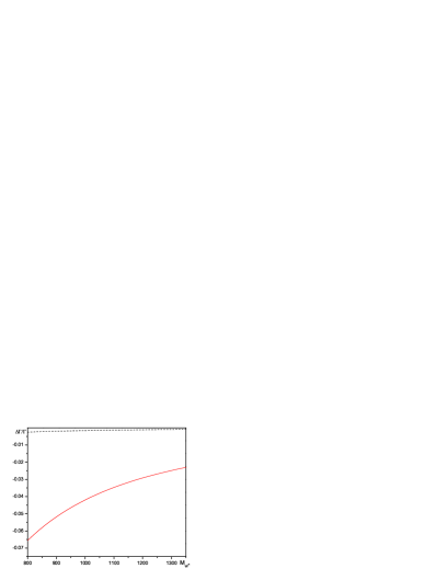
(a) Dependence of $\Delta\Gamma_{B_{s}}/\Gamma_{s}$ on $M_{W}^{(R)}$. Solid line: non-manifest LRSM ($\kappa=1$), dashed line: manifest LRSM.

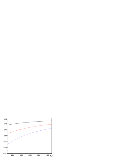
(b) Dependence of $\Delta\Gamma_{B_{s}}/\Gamma_{s}$ on $M_{W}^{(R)}$ in non-manifest LRSM. Solid line: $\kappa=1$, dashed line: $\kappa=1.5$, dotted line: $\kappa=2$.

Figure 5: Contributions to $\Delta\Gamma_{B_{s}}/\Gamma_{s}$ in the Left-Right Symmetric Models.

V Conclusions

We computed the subleading $1/m_{b}^{2}$ corrections to the difference in the lifetimes of $B_{s}$ mesons. We showed that they can be parameterized by 13 nonperturbative parameters, which we denote $\alpha_{i}$ and $\beta_{i}$. We adopted the statistical approach for presenting our results and generate 100000-point probability distributions of the lifetime difference, obtained by randomly varying our parameters within a $\pm 30\%$ interval around their “factorization” values, except for the case when the parameters are known from lattice QCD. In this case they are taken to vary within a $1\sigma$ interval as indicated above.

The results are presented in Fig. (3). While there is no theoretically-consistent way to translate the histogram of Fig. 3 into numerical predictions for $\Delta\Gamma_{B_{s}}/\Gamma_{s}$, we provide an estimate by taking the width of the distribution Fig. 3 at the middle of its height as 1-$\sigma$ variance and position of the maximum of the curve as the most probable value,

$$\Delta\Gamma_{B_{s}}=0.072^{+0.034}_{-0.030}~{}\mbox{ps}^{-1},\quad\frac{\Delta\Gamma_{B_{s}}}{\Gamma_{B_{s}}}=0.104\pm 0.049,$$ (54)

The effects of $1/m_{b}^{2}$ corrections to calculations of $\Delta\Gamma_{B_{s}}$ are shown to be small.

We also looked into $\Delta B=1$ New Physics contribution to the lifetime difference in the $B_{s}$ system. We have shown that these contributions can both enhance or reduce the Standard Model contribution. We considered the most general four-fermion effective Hamiltonian, which can be generated by any reasonable extension of the Standard Model and derived its contribution to $\Delta\Gamma_{B_{s}}$. We then evaluated effects of charged Higgses and right-handed W’s on the lifetime difference. While the contribution of charged Higgs was shown to be negligible in $\Delta\Gamma_{B_{s}}$, LRSM can be constrained with measurement of $\Delta\Gamma_{B_{s}}$, provided lattice or QCD sum rule community provide better estimates of non-perturbative parameters entering the SM calculation of the lifetime difference in $B_{s}$ mesons.

References

- (1) A. Abulencia et al. [CDF Collaboration], Phys. Rev. Lett. 97, 242003 (2006) [arXiv:hep-ex/0609040].
- (2) V. M. Abazov et al. [D0 Collaboration], Phys. Rev. Lett. 97, 021802 (2006) [arXiv:hep-ex/0603029].
- (3) J. G. Korner, A. I. Onishchenko, A. A. Petrov and A. A. Pivovarov, Phys. Rev. Lett. 91, 192002 (2003) [arXiv:hep-ph/0306032]; S. Narison and A. A. Pivovarov, Phys. Lett. B 327, 341 (1994) [hep-ph/9403225].
- (4) E. Dalgic et al., arXiv:hep-lat/0610104.
- (5) D. Becirevic, V. Gimenez, G. Martinelli, M. Papinutto, and J. Reyes, JHEP 0204, 025 (2002) [hep-lat/0110091].
- (6) V. Gimenez and J. Reyes, Nucl. Phys. Proc. Suppl. 94 (2001) 350 [hep-lat/0010048].
- (7) S. Aoki et al. [JLQCD Collaboration], arXiv:hep-ph/0307039; S. Aoki et al. [JLQCD Collaboration], Phys. Rev. D 67 (2003) 014506 [hep-lat/0208038].
- (8) V. M. Abazov et al. [D0 Collaboration], Phys. Rev. Lett. 98, 121801 (2007) [arXiv:hep-ex/0701012].
- (9) D. Acosta et al. [CDF Collaboration], Phys. Rev. Lett. 94, 101803 (2005) [arXiv:hep-ex/0412057].
- (10) R. Barate et al. [ALEPH Collaboration], Phys. Lett. B 486, 286 (2000).
- (11) W. M. Yao et al. [Particle Data Group], J. Phys. G 33 (2006) 1.
- (12) E. Barberio et al. [Heavy Flavor Averaging Group (HFAG) Collaboration], arXiv:0704.3575 [hep-ex].
- (13) M. Beneke, G. Buchalla, and I. Dunietz, Phys. Rev. D 54, 4419 (1996). M. Beneke, G. Buchalla, A. Lenz, and U. Nierste, Phys. Lett. B 576, 173 (2003).
- (14) M. Beneke, G. Buchalla, C. Greub, A. Lenz, and U. Nierste, Phys. Lett. B 459, 631 (1999) [arXiv:hep-ph/9808385].
- (15) M. Ciuchini, E. Franco, V. Lubicz, F. Mescia, and C. Tarantino, JHEP 0308, 031 (2003) [arXiv:hep-ph/0308029].
- (16) A. Lenz and U. Nierste, arXiv:hep-ph/0612167.
- (17) Y. Grossman, Y. Nir and G. Paz, Phys. Rev. Lett. 97, 151801 (2006) [arXiv:hep-ph/0605028].
- (18) Z. Ligeti, M. Papucci and G. Perez, Phys. Rev. Lett. 97, 101801 (2006) [arXiv:hep-ph/0604112].
- (19) Y. Grossman, Phys. Lett. B 380, 99 (1996) [arXiv:hep-ph/9603244].
- (20) I. Dunietz, R. Fleischer and U. Nierste, Phys. Rev. D 63, 114015 (2001) [arXiv:hep-ph/0012219].
- (21) G. Buchalla, A. J. Buras, and M. E. Lautenbacher, Rev. Mod. Phys. 68, 1125 (1996) [arXiv:hep-ph/9512380].
- (22) M. A. Shifman and M. B. Voloshin, Sov. J. Nucl. Phys. 41, 120 (1985) [Yad. Fiz. 41, 187 (1985)].
- (23) F. Gabbiani, A. I. Onishchenko, and A. A. Petrov, Phys. Rev. D 70, 094031 (2004) [arXiv:hep-ph/0407004]. F. Gabbiani, A. I. Onishchenko, and A. A. Petrov, Phys. Rev. D 68, 114006 (2003).
- (24) “Lifetimes and lifetime differences in heavy mesons,” talk given by A. A. Petrov at 33rd International Conference on High Energy Physics (ICHEP 06), Moscow, Russia, 26 Jul - 2 Aug 2006.
- (25) M. Beneke, G. Buchalla, M. Neubert and C. T. Sachrajda, Phys. Rev. Lett. 83, 1914 (1999) [arXiv:hep-ph/9905312]; C. W. Bauer, S. Fleming, D. Pirjol and I. W. Stewart, Phys. Rev. D 63, 114020 (2001) [arXiv:hep-ph/0011336].
- (26) E. Golowich, S. Pakvasa and A. A. Petrov, Phys. Rev. Lett. 98, 181801 (2007) [arXiv:hep-ph/0610039].
- (27) S. L. Glashow and S. Weinberg, Phys. Rev. D 15, 1958 (1977).
- (28) V. D. Barger, J. L. Hewett and R. J. N. Phillips, Phys. Rev. D 41, 3421 (1990).
- (29) D. Atwood, L. Reina and A. Soni, Phys. Rev. D 55, 3156 (1997) [arXiv:hep-ph/9609279].
- (30) E. Golowich and T.Yang, Phys. Lett B 80, 245 (1979)
- (31) R. N. Mohapatra and J. C. Pati, Phys. Rev. D 11, 2558 (1975); For a review and complete set of original references, see R. N. Mohapatra, “UNIFICATION AND SUPERSYMMETRY. THE FRONTIERS OF QUARK - LEPTON PHYSICS,” Berlin, Germany: Springer ( 1986) 309 p. (Contemporary Physics)
- (32) K. Kiers, M. Assis and A. A. Petrov, Phys. Rev. D 71, 115015 (2005) [arXiv:hep-ph/0503115].
- (33) G. Beall, M. Bander and A. Soni, Phys. Rev. Lett. 48, 848 (1982).
- (34) F. I. Olness and M. E. Ebel, Phys. Rev. D 30, 1034 (1984).
- (35) D. Chang, R. N. Mohapatra and M. K. Parida, Phys. Rev. D 30, 1052 (1984).
- (36) E. Golowich, J. Hewett, S. Pakvasa and A. A. Petrov, arXiv:0705.3650 [hep-ph].