Fractal valence bond loops in a long-range Heisenberg model at criticality

Abstract

We present a valence bond theory of the spin-$S$ quantum Heisenberg model. For nonfrustracting, local exchange and dimension $d>1$, it predicts a resonating ground state with bond amplitudes $h(r)\sim(a^{2}+r^{2})^{-p/2}$ and decay exponent $p=d+1$. Different values of $p$ can be achieved by introducing frustrating ($p>d+1$) or nonfrustrating ($p<d+1$) long-range interactions. For $d=2$, but not $d=3$, there is a critical value of the decay exponent $p_{\text{c}}$ above which the ground state is a spin liquid. The phase transition is analogous to quantum percolation, with fractal valence bond loops playing the role of percolating clusters. The critical exponents are continuously tunable along the phase boundary $p=p_{\text{c}}(a,S)$.

Singlet product states were introduced in the early days of quantum chemistry to describe valence bonding in molecules Rumer32 ; Pauling33 . These “valence bond states” were also applied to translationally invariant systems and proved especially useful for studying interacting $S=\tfrac{1}{2}$ quantum spin chains Hulthen38 ; Majumdar69 . A featureless resonating valence bond (RVB) wavefunction, consisting of a superposition of all possible configurations of short range valence bonds, was later promoted by Anderson as a possible ground state for low-coordination-number antiferromagnets Anderson73 ; Fazekas74 and as a potential route to superconductivity in the cuprates Anderson87a ; Kivelson87a .

Liang, Doucot, and Anderson (LDA) extended the RVB picture to include bonds on all length scales by assuming that the weight associated with each configuration could be factorized into a product of individual bond amplitudes, each expressed as a single function of the bond length Liang88 . They considered various functional forms for the two-dimensional Heisenberg model and concluded that the optimal amplitudes fall off as a powerlaw: $h(r)\sim r^{-p}$. Their variational calculation was not sufficiently accurate to resolve the correct exponent, which is almost certainly $p=3$ Sandvik05 ; Lou06 ; Havilio99 .

In this Letter, we begin by providing a formal justification for the LDA ansatz. The calculation presented here is a mean field treatment of the Heisenberg model based on valence bond creation and annihilation operators Beach06 ; these obey an unusual operator algebra that reproduces the properties of the overcomplete valence bond basis. We show that a broad class of spin-$S$ models with two-spin interactions have ground state wavefuctions that are very close to being factorizable-amplitude RVB states. Antiferromagnetically ordered states attain perfect factorizability in the large spin limit.

For models with local, nonfrustrating interactions, the mean field equations can be solved analytically. The amplitudes are generically radially symmetric and of the form $h(r)=(a^{2}+r^{2})^{-p/2}$, where the core size of the distribution is $a=1/\sqrt{d}$ and the powerlaw tail has exponent $p=d+1$. Here $d$ is the dimension of the lattice. The only exception is for $d=1$, in which case either the bond lengths are gaussian distributed (even $2S$) or beyond mean field prediction (odd $2S$). In summary,

$$h(r) =\frac{2}{\sqrt{\pi}}\biggl{[}\frac{\xi-1}{\xi(\xi+1)}\biggr{]}^{\!1/2}\!e^{-r^{2}/2\xi^{2}} \quad d =1,\,\text{$2S$ even}$$ (1)

$$h(r) =\frac{1}{\pi(\frac{1}{2}+r^{2})^{3/2}} d =2$$ (2)

$$h(r) =\frac{2\sqrt{6}}{3\pi^{2}(\frac{1}{3}+r^{2})^{2}} d =3$$ (3)

The $\xi$ appearing in Eq. (1) is the spin correlation length

$$\xi^{2}=1+\frac{1}{\pi^{2}}e^{\pi(2S+1)}.$$ (4)

We then ask the question, are there couplings $J_{ij}$ that preserve the $h(r)=(a^{2}+r^{2})^{-p/2}$ form but accommodate arbitrary values of $p$ ? Indeed, it turns out that tuning $p$ away from $d+1$ is equivalent to introducing a long-range, bipartite interaction ($i,j$ in opposite sublattices)

$$J_{ij}=\gamma_{ij}+\bigl{(}1-\gamma_{ij}\bigr{)}\frac{\beta(p)(d+1-p)}{r_{ij}^{\alpha(p)}},$$ (5)

where $\gamma_{ij}$ is the nearest neighbour matrix and $\alpha(p),\beta(p)$ are smooth, positive functions. The beyond-nearest-neighbour part is frustrating when $\delta p=p-d-1>0$. For the square lattice, $\alpha(3+\delta p)=4+0.84\,\delta p$ and $\beta(3+\delta p)=0.7-0.15\,\delta p$.

The function $h(r)=(a^{2}+r^{2})^{-p/2}$ characterizes a family of RVB states interpolating between the classical Néel state ($p\to 0$) and Anderson’s short-range RVB state ($p\to\infty$). For $d=2$, these two limits are separated by a phase transition: there is a critical line $p=p_{\text{c}}(a,S)$ beyond which the system is quantum disordered. See Fig. 1. Along the critical line, the valence bond loops are scale invariant and have fractal dimension $D_{f}$. Their length distribution is characterized by entropy and loop tension exponents, $\tau(a,S)$ and $\sigma(a,S)$, in terms of which all other critical exponents can be expressed. In higher dimensions, where even the short-range RVB state is Néel ordered, there is no transition.

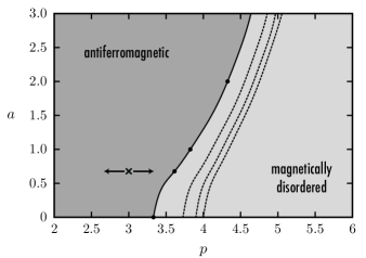
Figure 1: A phase diagram for the RVB wavefunction with amplitudes $h(r)=(a^{2}+r^{2})^{-p/2}$ on the square lattice. $r$ is the length of a valence bond connecting spins in opposite sublattices. The phase boundary is drawn for $S=\tfrac{1}{2}$ (solid line) and for $S=1,\tfrac{3}{2},2$ (dotted lines, from left to right). The location of the ground state ($\times$) can be adjusted horizontally by perturbing [as per Eq. (5)] about the nearest-neighbour Heisenberg model. Points at which the critical exponents have been measured (see Table 1) are marked ($\bullet$).

Mean field—The valence bond creation and annihilation operators $\chi^{\mu\dagger}_{ij}$ and $\chi^{\mu}_{ij}$, discussed in Ref. Beach06, , form an overcomplete basis for any system consisting of an even number of SU(2) spins. The operator $\chi^{\mu\dagger}_{ij}=(\chi^{0\dagger}_{ij},\bm{\chi}^{\dagger}_{ij})$ creates a singlet ($\mu=0$) or triplet ($\mu=1,2,3$) pair at sites $i$ and $j$ out of the spinless vaccuum. More precisely,

$$\chi^{\mu\dagger}_{ij}\lvert\text{vac}\rangle=\sum_{s,s^{\prime}=\uparrow,\downarrow}\tau^{\mu}_{s,s^{\prime}}\lvert s\rangle_{i}\otimes\lvert s^{\prime}\rangle_{j},$$ (6)

where $\tau^{\mu}=(\mathrm{i}\sigma^{2},\mathrm{i}\sigma^{3},\mathbb{1},-\mathrm{i}\sigma^{1})$ is a vector of $2\times 2$ matrices related to the Pauli matrices by $\tau^{0}=\mathrm{i}\sigma^{2}$ and $\bm{\tau}=\bm{\sigma}\sigma^{2}$.

Valence bond operators with no indices in common commute. Those with matching site indices obey a bosonic commutation relation, whereas those with only one index in common obey a more complicated rule:

$$\bigl{[}\chi^{\mu}_{ij},\chi^{\nu\dagger}_{ij}\bigr{]}\lvert\text{vac}\rangle =\delta^{\mu\nu}\lvert\text{vac}\rangle,$$ (7)

$$\bigl{[}\chi^{\mu}_{ij},\chi^{\rho\dagger}_{kj}\chi^{\theta\dagger}_{il}\bigr{]}\lvert\text{vac}\rangle =\frac{1}{2}\sum_{\nu}T^{\nu\rho\mu\theta}\chi^{\nu\dagger}_{kl}\lvert\text{vac}\rangle.$$ (8)

Here, $T^{\nu\rho\mu\theta}=\frac{1}{2}\operatorname{tr}\tau^{\nu\dagger}\tau^{\rho}\tau^{\mu\dagger}\tau^{\theta}$ takes the values $0,\pm 1$. Equation (8) encodes the overcompleteness of the basis.

Valence bond operators can be used to construct higher-spin states, so long as there are exactly $2S$ bonds emerging from each site: $\sum_{\mu}\chi^{\mu\dagger}_{ij}\chi^{\mu}_{ij}=2S$. Then each valence bond state is characterized by a set $v$ specifying the endpoints and singlet/triplet character of each bond. That is, $\lvert v\rangle=\mathcal{S}\bigl{[}\prod\chi^{\mu\dagger}_{ij}\bigr{]}\lvert\text{vac}\rangle$, where the product is over all $(i,j,\mu)\in v$ and $\mathcal{S}$ denotes a symmetrization of the operators with respect to all orderings Affleck87 ; Liang90 .

Since singlet bonds have a direction associated with them ($\chi^{0}_{ji}=-\chi^{0}_{ij}$, whereas $\bm{\chi}_{ji}=\bm{\chi}_{ij}$), we restrict our discussion to bipartite lattices ($N$ spins in each sublattice) and adopt the convention that all bonds originate in the $A$ sublattice and terminate in the $B$ sublattice. Hence, operator indices appear in the standard order $\chi^{\mu\dagger}_{ij}$ with $i\in A$ and $j\in B$, and the transform $\chi^{\mu}_{\mathbf{q}}$ is defined at only $N$ wavevectors in a reduced Brioullin zone.

An arbitrary state can be expressed as a linear combination (not unique) $\lvert\psi\rangle=\sum_{v}\psi(v)\rvert v\rangle$. Factorizability in the LDA sense means that the coefficient $\psi(v)=\prod a_{ij}^{\mu}$ can be decomposed into a product of individual bond amplitudes $a^{\mu}_{ij}$. Even under the assumption of perfect factorization, this wavefunction is nontrivial, since there are geometrical constraints implicit in tiling the lattice with hard-core dimers.

Those constraints can be made explicit in the following way. The bond configuration sum can be achieved by exponentiation of a weighted one-bond operator:

$$\lvert\psi\rangle=\hat{G}\exp\sum_{i\in A}\sum_{j\in B}\sum_{\mu}a^{\mu}_{ij}\chi^{\mu\dagger}_{ij}\lvert\text{vac}\rangle.$$ (9)

The Gutzwiller projection operator $\hat{G}=\prod_{i\in A}\delta(\hat{N}_{i}-2S)$ filters out all configurations that do not have exactly $2S$ bonds emerging from each lattice site. This is similar in spirit to the construction of Anderson’s projected BCS wavefunction Anderson87a , but here the underlying operators are not paired fermions. The projection step can be implemented by introducing a gauge field at each bond endpoint: $\chi^{\mu\dagger}_{ij}\to e^{\mathrm{i}\pi(\phi_{i}+\phi_{j})}\chi^{\mu\dagger}_{ij}$ and $\hat{G}=\int\!D[\phi]\,e^{-\mathrm{i}\sum_{j}2\pi S\phi_{j}}$.

Equation (9) can be written compactly as $\rvert\psi\rangle=\hat{G}\rvert a\rangle$ with $\rvert a\rangle=\exp\sum_{\mathbf{q},\mu}a_{\mathbf{q}}^{\mu}\chi^{\mu\dagger}_{\mathbf{q}}\lvert\text{vac}\rangle$. If we relax $\hat{G}$ and enforce the number constraint on average (fixing the overall bond number at $2SN$), then $\rvert a\rangle$ can be viewed as a mean field approximation to $\rvert\psi\rangle$. Since $\hat{N}_{i}\sim\partial/\partial\phi_{i}$, the total bond number operator $\hat{N}=\sum_{i\in A}\hat{N}_{i}$ is related to the overall normalization of the bond amplitudes:

$$\hat{N}\lvert a\rangle=\frac{\partial}{\partial u}\lvert ua\rangle\Bigr{\rvert}_{u=1}=\sum_{\mathbf{q},\mu}a^{\mu}_{\mathbf{q}}\chi^{\mu\dagger}_{\mathbf{q}}\lvert a\rangle.$$ (10)

Let us assume that the spin-spin interactions in the Hamiltonian act only between sites in opposite sublattices: $\hat{H}=\sum_{i\in A}^{j\in B}J_{ij}\mathbf{S}_{i}\cdot\mathbf{S}_{j}-\lambda(\hat{N}-N)$. We have introduced a Lagrange multiplier $\lambda$ coupled to the shift in bond number. In the state $\rvert a\rangle$, the valence bond operator has an anomalous expectation value $\Delta^{\mu}_{ij}=J_{ij}\langle\chi^{\mu}_{ij}\rangle$. For a singlet ground state, the various triplet components vanish: $\Delta^{\mu}_{\mathbf{q}}=\Delta^{0}_{\mathbf{q}}\delta^{\mu,0}\sim JS\delta^{\mu,0}$ and $a^{\mu}_{\mathbf{q}}=h_{\mathbf{q}}\delta^{\mu,0}$. The expectation value of $\mathbf{S}_{i}\cdot\mathbf{S}_{j}$ between valence bond states depends on whether $i$ and $j$ are in the same valence bond loop Liang88 . At the mean field level,

$$\mathcal{C}_{ij}=(-1)^{i+j}\bigl{\langle}\mathbf{S}_{i}\cdot\mathbf{S}_{j}\bigr{\rangle}=\frac{1}{2}\bigl{\lvert}X_{ij}\bigr{\rvert}^{2}-(S+1)\delta_{ij},$$ (11)

where $X_{ij}=\mathsf{F}[h_{\mathbf{q}}/\bigl{(}1-\tfrac{1}{2}\lvert h_{\mathbf{q}}\rvert^{2}\bigr{)}]$ and $X_{ik}=\mathsf{F}[\sqrt{2}/\bigl{(}1-\tfrac{1}{2}\lvert h_{\mathbf{q}}\rvert^{2}\bigr{)}]$ (with $i,k\in A$ and $j\in B$) measure the probability that two sites are connected by a chain of bonds. By the variational principle, $\partial\langle H\rangle/\partial h_{\mathbf{q}}^{*}=0$ yields

$$\langle\chi^{0}_{\mathbf{q}}\rangle=\frac{h_{\mathbf{q}}}{1-\frac{1}{2}\lvert h_{\mathbf{q}}\rvert^{2}}=\frac{\Delta_{\mathbf{q}}^{0}}{\omega_{\mathbf{q}}},\ \ \omega_{\mathbf{q}}=\sqrt{\lambda^{2}-2|\Delta^{0}_{\mathbf{q}}|^{2}},$$ (12)

and $\partial\langle H\rangle/\partial\lambda=0$ yields

$$\frac{1}{N}\sum_{\mathbf{q}}\frac{\lambda}{\omega_{\mathbf{q}}}=1+2S.$$ (13)

If $J_{ij}=J\gamma_{ij}$, the dispersion is $\omega_{\mathbf{q}}=(\epsilon^{2}+1-\gamma_{\mathbf{q}}^{2})^{1/2}$, in units where $|\Delta_{\mathbf{q}=0}^{0}|=1/\sqrt{2}$ and $\lambda^{2}=1+\epsilon^{2}$. In $d=1$, there is an important difference between integer and half-integer values of $S$ Haldane85 . For even $2S$, excitations are gapped and Eq. (13) reads $-\frac{2}{\pi}\log\frac{\epsilon}{\pi}=2S+1$, which leads to Eq. (1). For odd $2S$, the mean field breaks down; the system is gapless Lieb61 , but $\omega_{q}\sim q$ causes the bond constraint equation to diverge. [The bosonization result, $X_{ij}\sim\sqrt{\mathcal{C}_{ij}}\sim r_{ij}^{1/2}(\log r_{ij})^{1/4}$ suggests $h(r)\sim r^{-3/2}(\log\log r+O(1))$]. For $d\geq 2$, however, the gap $\epsilon=O(L^{-d})$ vanishes faster than the wavevector spacing $\pi/L$. Thus, as $L\to\infty$, the divergence in the bond number equation is confined to the zero mode and the stucture of the equation mimics that of so-called “sublattice-symmetric spinwave theory” Hirsch88 :

$$\frac{1}{N}\sum_{\mathbf{q}}\frac{\lambda}{\omega_{\mathbf{q}}}\to\frac{1}{N\epsilon}+c=1+2S.$$ (14)

The details of the lattice enter as a single geometrical constant, $c\doteq 1.393$ (square), $c\doteq 1.1567$ (cubic), etc. The staggered moment extracted from the large separation limit of $X_{ij}=\langle\chi^{0}_{ij}\rangle$ is $M=S-\frac{1}{2}(c-1)$, the usual spinwave result Anderson52 . $\epsilon\to 0$ leads to the long-wavelength behaviour $\log(h_{\mathbf{q}}/\sqrt{2})=-q/\sqrt{d}+O(q^{3})$, with deviations from radial symmetry not appearing until $O(q^{4})$. The corresponding real-space bond amplitudes for $d=2,3$ [Eqs. (2) and (3)] are found by computing the Hankel transform. In general, the presence of gapless, linearly dispersive excitations implies $h(r)\sim 1/r^{d+1}$. The core size $a=1/\sqrt{d}=\sqrt{2}v_{\text{s}}/\lvert\Delta^{0}_{\mathbf{q}=0}\rvert$ is proportional to the spin-wave velocity $v_{\text{s}}$.

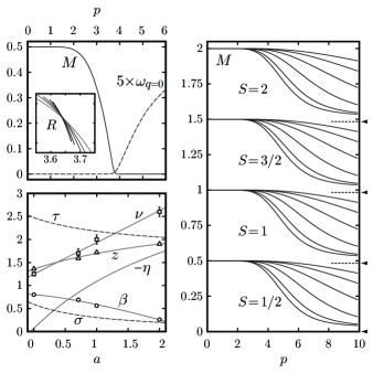
Figure 2: (Top-left) The staggered moment $M$ and spin gap $\omega_{\mathbf{q}=0}$ on a square lattice of size $L=192$ are plotted for $2S=1$, $a=1/\sqrt{2}$. The critical value $p_{\text{c}}=3.6256(5)$ is determined from crossing points of the ratio $R=X(\tfrac{L}{2},\tfrac{L}{2})/X(\tfrac{L}{4},\tfrac{L}{4})$; the curves $L=64,96,128,192,256$ are shown in the inset. (Bottom-left) Critical exponents $\nu$ ($\square$), $\beta$ ($\fullmoon$), and $z$ ($\triangle$) for $2S=1$ are plotted alongside the predicted values (solid lines) of the exponents based on a [1,1]-Padé approximant fit of $\tau$ and $\sigma$ (dashed lines). (Right) The staggered moment on the $L=32$ cubic lattice is shown for $2S=1,2,3,4$ and $2a=0,1,\ldots,5$. In the limit $L,p,1/a\to\infty$, its value bottoms out at $M_{\infty}=S-0.52$, indicated by dotted lines and an arrow.

We now consider the broader class of wavefunctions with amplitudes $h(r)=\bigl{(}a^{2}+r^{2}\bigr{)}^{-p/2}$ and compute the corresponding $p$–$a$ phase diagram. In the $d=2$ case (Fig. 1), there is a quantum disordered phase at sufficiently large $p$ for all values of $a$ and $S$. The critical exponents ($\beta,\nu,z$ can be measured directly; see Fig. 2) vary continuously and monotonically along the line of transitions with $\beta\!\nearrow\!0.8$, $\nu\!\searrow\!1.25$, and $z\!\searrow\!1.36$ as $a\!\searrow\!0$. The loss of long range order can be attributed to a qualitative change in the distribution of valence bond loops—a vanishing number of system-spanning loops on the magnetic side becomes a macroscopic number of small loops on the spin liquid side Beach06 . At criticality, the problem is formally equivalent to that of percolation, with self-similar valence bond loops of fractal dimension $D_{f}=d-\beta/\nu$ Gefen81 playing the role of percolating clusters (although loops, unlike clusters, are all backbone, i.e., free of dangling spins Wang06 ); fluctuations of the loop gas substitute for the geometric average over disorder configurations. More precisely, the analogy is with quantum, rather than classical percolation: the bare dynamical exponent $z_{0}=1$ should be renormalized according to $z=\phi D_{f}=D_{f}$, where $\phi=z_{0}/(2-z_{0})=1$ Vojta05 . This is borne out by measurements of the critical exponents, listed in Table 1.

Near criticality, the loops are distributed according to $n_{l}\sim l^{-\tau}\exp[-(p_{\text{c}}-p)^{1/\sigma}l]$, $n_{l}$ being the number of loops of length $l$. The distribution is parameterized by an entropy exponent $\tau$ and a loop tension exponent $\sigma$, which are related to the conventional exponents by $\nu=(\tau-1)/d\sigma$, $\beta=(\tau-2)/\sigma$, and $z=D_{f}=d/(\tau-1)$. The bottom-left panel of Fig. 2 illustrates the excellent agreement between measured exponents and their predicted values based on a [1,1]-Padé fitting form for $\tau$ and $\sigma$. Note that the anomalous dimension, determined from the relation $\eta=2\beta/\nu-z+2-d$, is strictly negative and goes as $\eta\approx-a$.

On the disordered side of the transition, the system is a gapped spin liquid. In the $p\to\infty$ limit, the short-range RVB state on the square lattice has a spin correlation function

$$\mathcal{C}_{ij}\sim S(S+1)\frac{e^{-r_{ij}/\xi}}{r_{ij}},$$ (15)

where $\xi(\tfrac{1}{2})\doteq 0.83$, $\xi(1)\doteq 2.0$, $\xi(\tfrac{3}{2})\doteq 4.4$, and $\log\xi(S)\sim 1.5\,S$ for large spin. In contrast, long-range antiferromagnetic order survives in $d=3$ for all $p$. This is true at the mean field level provided that $S>\tfrac{1}{2}$ (see Fig. 2); a direct evaluation of the short-range RVB ground state (using an efficient valence bond worm algorithm) confirms that the $S=\tfrac{1}{2}$ case is also Néel ordered.

Table 1: Critical exponents — $S=\tfrac{1}{2}$, square lattice

$a$	$p_{\text{c}}$	$\nu$	$\beta$	$z$	$D_{f}$
0	3.3677(2)	1.25(4)	0.80(2)	1.361(7)	1.36(3)
$1/\sqrt{2}$	3.6256(5)	1.7(1)	0.69(4)	1.594(6)	1.59(3)
1	3.800(1)	2.0(1)	0.56(3)	1.718(6)	1.72(2)
2	4.24(1)	2.6(1)	0.26(1)	1.902(4)	1.90(5)

We now run the mean field equations in reverse and solve, via

$$\frac{\Delta_{\mathbf{q}}^{0}}{\lambda}=\frac{h_{\mathbf{q}}}{1+\frac{1}{2}{\lvert h_{\mathbf{q}}\rvert^{2}}},\quad\frac{J_{ij}}{\lambda}=\frac{\mathsf{F}[\Delta_{\mathbf{q}}^{0}/\lambda]}{\mathsf{F}[\langle\chi^{0}_{\mathbf{q}}\rangle]},$$ (16)

for the interaction that stabilizes ground states with $a=1/\sqrt{d}$ and arbitrary $p$ (parameterizing, e.g., the horizontal trajectory in Fig. 1). The result is the interaction given in Eq. (5). Numerical estimates on the square lattice show that the long-range part goes as $[0.83(4-\alpha)+0.21(4-\alpha)^{2}+\cdots]/r_{ij}^{\alpha}$. The solutions are characterized by $\omega_{\mathbf{q}}\sim 1/\langle\chi^{0}_{\mathbf{q}}\rangle\sim q^{\theta}$ and $1-\Delta^{0}_{\mathbf{q}}\sim q^{2\theta}$, where $\theta=1+(\alpha-4)+O(\alpha-4)^{2}\approx\alpha-3$. For nonfrustrating interactions ($\alpha<4$), the dispersion is sublinear and for frustrating interactions ($\alpha>4$), it is superlinear. As the excitations soften, there is a point ($d=2$ only) at which the zero mode of the constraint equation ceases to hold macroscopic weight. Here, the magnetic order vanishes and a gap opens in the excitation spectrum. For $S=\tfrac{1}{2}$, that point occurs at $\theta_{\text{c}}\doteq 1.5$ and at large $S$, $\theta_{\text{c}}\approx 2-\tfrac{1}{4\pi^{2}S}$. Oddly, Eq. (5) (with $J_{ij}\sim-3.6/r_{ij}^{4.6}$) takes us up to but not through this critical point. Entry into the $p>p_{\text{c}}$ phase corresponds to the development of an unusual concentric-ringed, cloverleaf pattern of alternating frustrating and nonfrustrating interactions, as shown in Fig. 3. Other Hamiltonians with tunable interaction strengths potentially lead to different trajectories in the $p$–$a$ plane.

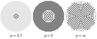
Figure 3: The sign of the exchange interaction $J_{ij}$ is plotted for $a=1/\sqrt{2}$ and various values of $p>p_{\text{c}}$. Dark dots denote $J_{ij}>0$ and light dots $J_{ij}<0$.

A key point is that the long-range, frustrating terms in Eq. (5) push $p$ to higher values (toward the disordered phase) while preserving the radial symmetry and positivity of $h(r)$. This is generally not true of short-range frustrating interactions, which tend to break the radial symmetry ($h(r)\to h(\mathbf{r})$) and, at large coupling strength, the Marshall sign rule ($\exists\,\mathbf{r}$ such that $h(\mathbf{r})<0$) Lou06 . Since reduction of the continuous rotational symmetry to the discrete rotational symmetry of the lattice is a precursor to crystalline bond ordering, preservation of the radial symmetry is important if the liquid state is not to be preempted by a bond ordered one.

The author gratefully acknowledges helpful discussions with Anders Sandvik, Valeri Kotov, and Fakher Assaad.

References

- (1) G. Rumer, Gottingen Nachr. Tech. 1932, 377 (1932).
- (2) L. Pauling, J. Chem. Phys. 1, 280 (1933).
- (3) L. Hulthén, Arkiv Mat. Astron. Fysik 26A, No. 11 (1938).
- (4) C. K. Majumdar and D. K. Ghosh, J. Math. Phys. 10, 1388 (1969).
- (5) P. W. Anderson, Mater. Res. Bull. 8, 153 (1973).
- (6) P. Fazekas and P. W. Anderson, Philos. Mag. 30, 23 (1974).
- (7) P. W. Anderson, Science 235, 1196 (1987).
- (8) S. A. Kivelson, D. S. Rokhsar, and J. P. Sethna, Phys. Rev. B 35, 8865 (1987).
- (9) S. Liang, B. Doucot, and P. W. Anderson, Phys. Rev. Lett. 61, 365 (1988).
- (10) A. W. Sandvik, Phys. Rev. Lett. 95, 207203 (2005).
- (11) J. Lou and A. W. Sandvik, arXiv:cond-mat/0605034v3.
- (12) M. Havilio and A. Auerbach, Phys. Rev. Lett. 83, 4848 (1999).
- (13) K. S. D. Beach and A. W. Sandvik, Nucl. Phys. B 750, 142 (2006).
- (14) J. E. Hirsch and S. Tang, Phys. Rev. B 39, 2850 (1989); ibid. 40, 4769 (1989).
- (15) P. W. Anderson, Phys. Rev. 86, 694 (1952).
- (16) I. Affleck, T. Kennedy, E. H. Lieb, and H. Tasaki, Phys. Rev. Lett. 59, 799 (1987).
- (17) S. Liang, Phys. Rev. Lett. 64, 1597 (1990).
- (18) F. D. M. Haldane, J. Appl. Phys. 57, 3359 (1985).
- (19) E. Lieb, T. Schultz, D. Mattis, Ann. Phys. (N.Y.) 16, 407 (1961).
- (20) Y. Gefen, A. Aharony, B. B. Mandelbrot, and S. Kirkpatrick, Phys. Rev. Lett. 47, 1771 (1981).
- (21) L. Wang and A. W. Sandvik, Phys. Rev. Lett. 97, 117204 (2006).
- (22) T. Vojta and J. Schmalian, Phys. Rev. Lett. 95, 237206 (2005).