The Nature of Stellar Winds in the Star-Disk Interaction

Abstract

Stellar winds may be important for angular momentum transport from accreting T Tauri stars, but the nature of these winds is still not well-constrained. We present some simulation results for hypothetical, hot ($\sim 10^{6}$ K) coronal winds from T Tauri stars, and we calculate the expected emission properties. For the high mass loss rates required to solve the angular momentum problem, we find that the radiative losses will be much greater than can be powered by the accretion process. We place an upper limit to the mass loss rate from accretion-powered coronal winds of $\sim 10^{-11}M_{\odot}$ yr^-1. We conclude that accretion powered stellar winds are still a promising scenario for solving the stellar angular momentum problem, but the winds must be cool (e.g., $~{}10^{4}$ K) and thus are not driven by thermal pressure.

1 Introduction

Observations (e.g., Herbst et al., 2007) reveal that a large fraction of accreting T Tauri stars (CTTSs) spin slowly, that is at $\sim 10$% of breakup speed. This is surprising because the accretion of disk material adds angular momentum to the star (e.g., Matt & Pudritz, 2007). One promising scenario to explain how the slowly spinning stars rid themselves of this accreted angular momentum, proposed by Hartmann & Stauffer (1989), is that a stellar wind carries it off. For this to work, the mass outflow rate should be approximately proportional to the accretion rate. Depending on the stellar magnetic field strength (among other things), in order to solve the stellar angular momentum problem, the wind outflow rate needs to be of the order of 10% of the accretion rate (Matt & Pudritz, 2005).

Since the “typical” mass accretion rate observed in the CTTSs is $\dot{M}_{\rm a}\sim 10^{-8}M_{\odot}$ yr^-1 (Johns-Krull & Gafford, 2002), this means the stellar wind should have a mass outflow rate of $\dot{M}_{\rm w}\sim 10^{-9}M_{\odot}$ yr^-1. A wind this massive requires a lot of power to accelerate it, and Matt & Pudritz (2005) suggested that a fraction of the potential energy liberated by the accretion process goes into driving the wind. In the case of a coronal wind (i.e., $\sim 10^{6}$ K, thermally driven), for example, this requires $\sim 10$% of the accretion power (Matt & Pudritz, 2005). There is some observational evidence for accretion-powered stellar winds in these systems (Edwards et al., 2006; Kwan et al., 2007).

But what is the nature of T Tauri stellar winds? How massive are they, and what drives them? The mass outflow rates of stellar winds is very poorly constrained observationally (e.g., Dupree et al., 2005). This is basically due to the extreme difficulty in disentangling the signatures of a stellar wind from signatures of a wind from the inner edge of a disk and a host of other energetic phenomena exhibited by CTTSs. The wind driving mechanism is also not constrained and is the primary focus of this paper.

2 The T Tauri Coronal Wind Hypothesis

T Tauri stars are magnetically active and possess hot, energetic corona (for a review, see Feigelson & Montmerle, 1999). They are 4–5 orders of magnitude more luminous in X-rays than the sun. Thus, it stands to reason that they drive solar-like coronal winds, but more powerful. In this case, the wind is primarily thermal pressure-driven, and the wind temperature needs to be $\sim 10^{6}$ K for the pressure force to overcome gravity. As a first step, we make the hypothesis here that some of the accretion power is transferred to heat in the stellar corona, and thus drives a coronal wind.

There is only one calculation in the literature (that we are aware of) that constrains the mass outflow rate of coronal winds from CTTSs. Specifically, Bisnovatyi-Kogan & Lamzin (1977) calculated the X-ray emission from coronal winds. From these calculations, Decampli (1981) concluded that, in order for the wind emission to be consistent with the observed X-ray luminosities, the outflow rate of a T Tauri coronal wind must be less than $\sim 10^{-9}M_{\odot}$ yr^-1. As discussed above, a wind this massive may still be important for angular momentum transport, and thus we proceed.

3 Coronal Wind Simulations

To calculate realistic wind solutions, we carried out 2.5D (axisymmetric) ideal magnetohydrodynamic (MHD) simulations of coronal winds. For simplicity, we did not include the accretion disk. We employ the numerical code and method described by Matt & Balick (2004). This allows us to obtain steady-state wind solutions for a Parker-like coronal wind (Parker, 1958), as modified by the presence of stellar rotation and a rotation-axis-aligned dipole magnetic field. We assume a polytropic equation of state ($P\propto\rho^{\gamma}$), with no radiative cooling. The fiducial parameters are given in table 1, adopted to represent values for a “typical” CTTS.

Table 1: Fiducial Stellar Wind Parameters

Parameter	Value
$M_{*}$	0.5 $M_{\odot}$
$R_{*}$	2.0 $R_{\odot}$
$B_{*}$ (dipole)	200 G
$f$	0.1
$\dot{M}_{\rm w}$	$1.9\times 10^{-9}M_{\odot}$ yr-1
$T_{\rm c}$	$1.3\times 10^{6}$ K
$\gamma$	1.40

In table 1, $M_{*}$ and $R_{*}$ are the stellar mass and radius; $B_{*}$ is the magnetic field strength of the dipole magnetic field at the surface and equator of the star; $f$ is the spin rate of the star, expressed as a fraction of the breakup rate; $T_{\rm c}$ is the temperature at the base of the corona; and $\gamma$ is the polytropic index.

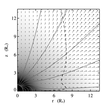
Figure 1: Greyscale of log density, velocity vectors, and magnetic field lines illustrate the structure of the steady-state wind solution for our fiducial case. The dashed line represents the Alfvén surface, where the wind speed equals the local Alfvén speed. The rotation axis is vertical, along the left side of the plot.

Figure 1 illustrates the steady-state wind solution for the fiducial case. We find that this wind carries away enough angular momentum to counteract the spin up torque from an accretion rate of $\dot{M}_{\rm a}\approx 5\times 10^{-9}M_{\odot}$ yr^-1. We also carried out a parameter study (Matt & Pudritz 2007, in preparation), which generally validates the idea that a stellar wind can indeed remove the accreted angular momentum in CTTSs.

4 Emission Properties of Coronal Wind

The simulation results of the previous section provide detailed solutions for the density and temperature in coronal stellar winds. Although the simulations did not include radiative cooling effects, it is instructive to examine the emission properties expected from these winds, ex post facto. For this, we employ the CHIANTI line database and IDL software (Dere et al., 1997; Landi et al., 2006), which allows us to calculate spectra and total radiative cooling rates in the wind.

The CHIANTI package assumes, among other things, that the ionization and excitation levels in the plasma are in a steady-state; all lines are optically thin; the plasma is in coronal equilibrium, so that the ionization state is in LTE. These assumptions are appropriate for the purposes of this work, and we also adopt cosmic abundances for the gas.

4.1 Illustrative Synthetic Spectrum

Figure 2: Synthetic spectrum of isothermal, $10^{6}$ K, optically thin coronal plasma. Flux units are arbitrary. The figure is generated by CHIANTI software.

For illustrative purposes, figure 2 shows a spectrum, computed by CHIANTI, of an isothermal plasma with a temperature of $10^{6}$ K. It is clear that the cooling is dominated by line emission. In this case, the three strongest emission lines (of Fe IX 171.1 Å, Fe X 174.5 Å, and Mg IX 368.1 Å) account for approximately $20$% of the total luminosity. Furthermore, only about 1% of the total energy is emitted shortward of 30 angstroms (i.e., in X-rays), and the vast majority of the emission is in the extreme UV.

4.2 Total Radiative Losses

CHIANTI also provides a tool to calculate the total cooling rate (i.e., radiated luminosity in erg s^-1; which is essentially an integration of the emission spectrum over wavelength, etc.) for any given coronal density, temperature, and emitting volume. With this, we calculate the cooling in each computational gridcell of our simulations, and sum over all gridcells, to obtain the total luminosity of the simulated wind solution. For the fiducial case, the total wind luminosity is a few times $10^{34}$ erg s^-1. Since optically thin emission is proportional to density squared, and since the mass outflow rate in the wind is approximately proportional to density, we express the luminosity of the wind as

$$L_{\rm w}\sim 10^{34}\;\;{\rm erg\;s}^{-1}\;\;\left({\dot{M}_{\rm w}\over 10^{-9}M_{\odot}{\rm\;yr}^{-1}}\right)^{2}.$$ (1)

As suggested by the example spectrum (fig. 2), if $\sim 1$% of this emission is emitted in X-rays, the X-ray luminosity of the wind is $\sim 10^{32}$ erg s^-1. This is significantly higher than the typically observed X-ray luminosity of CTTSs of $\sim 10^{30}$ erg s^-1 (Feigelson & Montmerle, 1999). Of course, we have calculated the total cooling rate, which is not exactly the observed luminosity. Consider that approximately half of this radiation will be blocked by the star, and there will likely be significant absorption of these soft X-rays. Still, it does not seem avoidable that the predicted X-ray luminosity from the fiducial coronal wind solution is much higher than typically observed.

4.3 Accretion Power

More importantly, we must consider the energy budget of the wind. The total cooling rate, $L_{\rm w}$, of the fiducial wind is two orders of magnitude larger than the kinetic energy in the wind ($0.5\dot{M}_{\rm w}v_{\infty}^{2}$, where $v_{\infty}^{2}$ is the wind speed)—this is approximately equivalent to saying that the cooling time is two orders of magnitude shorter than the wind acceleration time. Thus, it takes a lot more energy to keep this plasma hot (while it radiates) than it does to accelerate the matter away from the star.

In the accretion-powered stellar wind scenario, the energy in the wind somehow derives from the gravitational potential energy released by accreting gas ($\sim GM_{*}\dot{M}_{\rm a}/R_{*}$). This accretion power, assuming the fiducial stellar mass and radius, can be expressed approximately as

$$L_{\rm a}\sim 10^{32}\;\;{\rm erg\;s}^{-1}\;\;\left({\dot{M}_{\rm a}\over 10^{-8}M_{\odot}{\rm\;yr}^{-1}}\right).$$ (2)

As discussed in section 1, in order for stellar winds to solve the angular momentum problem, torque balance requires $\dot{M}_{\rm w}/\dot{M}_{\rm a}\sim 0.1$. Thus, if we fix this ratio of mass flow rates, it is clear from equations 1 and 2 that there is not enough accretion energy to keep coronal winds hot, in the fiducial case.

4.4 An Upper Limit on T Tauri Coronal Winds

If we fix the ratio $\dot{M}_{\rm w}/\dot{M}_{\rm a}\sim 0.1$, it is evident from equations 1 and 2 that there will be enough accretion power to drive a coronal wind when the wind outflow rate is

$$\dot{M}_{\rm w}\;\;{}^{<}_{\sim}\;\;10^{-11}\;\;M_{\odot}\;{\rm yr}^{-1}.$$ (3)

Thus, in principle, accretion-powered coronal winds can remove the accreted angular momentum for $\dot{M}_{\rm a}\sim 10^{-10}M_{\odot}$ yr^-1. However, for accretion rates this low, the spin up torque from accretion is so small that the time for the star to spin up from this torque is comparable to the entire pre-main-sequence lifetime (e.g., Matt & Pudritz, 2007). In other words, for these low accretion rates, there is no angular momentum problem. The logical conclusion is that, in order for accretion-powered stellar winds to solve the angular momentum problem, the winds cannot be as hot as we have considered here.

5 On the Validity of Our Simulated Wind Solutions

We showed in section 4 that the expected emission properties of our fiducial, coronal winds effectively rules them out. In other words, our assumption in this paper that the wind is driven by thermal-pressure is not realistic. However, it is important to note that the angular momentum carried in the wind does not depend on what drives the wind. Instead, the angular momentum outflow rate depends only on $B_{*}$, the rotation rate, $\dot{M}_{\rm w}$, $R_{*}$, and the wind velocity. As long as “something” accelerates the wind to speeds similar to what we see in our simulations (of the order of the escape speed), the torque we calculate is approximately correct.

For example, if the wind is cold and driven by Alfvén waves, the driving force can be parameterized as being proportional to $-\nabla\xi$ (where $\xi$ is the wave energy density; Decampli, 1981). This has the same functional form as the thermal-pressure force ($-\nabla P$) used in our simulations, so there is some form of $\xi$ that will result in a wind solution with exactly the same density and kinematics as our simulations (but a different temperature).

Thus, while the thermodynamic properties of our simulations have been invalidated, the conclusion that stellar winds are capable of carrying off accreted angular momentum is not affected.

6 Conclusion

Based on the emission properties of $\sim 10^{6}$ K coronal plasmas, we rule out hot coronal winds as a likely candidate for accretion-powered stellar winds. The coronal wind hypothesis fails. Instead, for mass loss rates comparable to our fiducial value of $10^{-9}M_{\odot}$ yr^-1, the winds must be as cool as $\sim 10^{4}$ K, where radiative cooling becomes much less efficient than for a coronal plasma. At temperatures this low, the pressure force cannot overcome the gravity of the star, and accretion-powered winds are thus not driven by thermal pressure.

To date, possibly the best observational evidence for accretion-powered stellar winds from CTTSs comes from measurements of blue-shifted absorption features in the He I emission line at 10830 Å (e.g., Edwards et al., 2003, 2006; Dupree et al., 2005). Furthermore, radiative transfer modeling by Kurosawa et al. (2006) suggests that a stellar wind may contribute significantly to the H$\alpha$ line profile. At densities where collisions between particles are important, both He I and H start to become substantially ionized at a temperature of a few times $10^{4}$ K. If the wind is much hotter than this, it may be difficult to explain the prominence of He I and H I features in observed spectra (see also Johns-Krull & Herczeg, 2007). Thus these works also support the conclusion that the winds are much cooler than a coronal plasma.

Accretion-powered stellar winds remain a promising scenario for solving the stellar angular momentum problem. But, the question remains, what is the nature of these winds? What drives them? Possible scenarios include Alfvén wave driving (Decampli, 1981), episodic magnetospheric inflation (Goodson et al., 1999; Matt et al., 2003), and reconnection X-winds (Ferreira et al., 2000, 2006).