Construction of equilibrium networks with an energy function

Abstract

We construct equilibrium networks by introducing an energy function depending on the degree of each node as well as the product of neighboring degrees. With this topological energy function, networks constitute a canonical ensemble, which follows the Boltzmann distribution for given temperature. It is observed that the system undergoes a topological phase transition from a random network to a star or a fully-connected network as the temperature is lowered. Both mean-field analysis and numerical simulations reveal strong first-order phase transitions at temperatures which decrease logarithmically with the system size. Quantitative discrepancies of the simulation results from the mean-field prediction are discussed in view of the strong first-order nature.

1 Introduction

Networks describe interaction patterns of various complex systems. In many cases, interactions switch constantly and their topology changes according to external conditions. If we treat a network as a thermodynamic system which has an energy function depending on its topology and introduce temperature as the disorder strength, networks constitute a topological ensemble of equilibrium networks of which physical quantities are described by methods of statistical mechanics [1, 2, 3]. At equilibrium, links are reallocated to satisfy the detailed balance and ergodicity; topological phase transitions are expected as the temperature is varied. Since there does not exist the physical energy of a network associated with its topology, the functional form of the energy is not given a priori: It may be taken as a function of the node degree, number of links, or some global property of the network. If an energy function is designed for certain performance, one can obtain an optimized network ensemble which minimizes the energy via zero-temperature dynamics. On the other hand, various topologies can be obtained at finite temperatures, with the entropy taken into account. A number of networks have been constructed through the use of energy functions with a focus on structural transitions [1, 4, 5] and optimization [6, 7]. In general, equilibrium networks constructed by a topological energy function are not complex but random [8] at high temperatures; they are rather simple at low temperatures as well, making either star or fully-connected networks. Exceptionally, scale-free networks come out only at the critical temperature if a logarithmic function of the degree is introduced for the energy [1]; this is logically obvious in view of that the corresponding rewiring dynamics reduces to the preferential attachment scheme.

In this study, we introduce a simple function of the degree as the energy function, which combines two competitive terms with different strengths, and examine the resulting topological phase transitions. Each term favors a different ground state, so one may expect various network topologies depending on the temperature and the relative strength.

There are five sections in this paper: Section 2 introduces the model, together with the energy function. In Sec. 3, the system is analyzed by means of the mean-field theory. Specifically, the energy and the entropy of the system are evaluated, in terms of which phase transitions between random, star, and fully-connected network phases are probed. Section 4 is devoted to numerical simulations. In particular the simulation results are discussed, in comparison with the mean-field results. Finally, a brief summary and concluding remarks are given in Sec. 5.

2 Model system

We consider a system of $N$ nodes, some of which are connected with each other. The total number of links is given by $M=(N/2)\langle k\rangle$, where $\langle k\rangle$ is the mean degree, i.e., the mean number of links per node. In this study, $\langle k\rangle$ is fixed to be $0.5$ and $M$ is kept conserved during rewiring.

Associated with the system is an energy function, which consists of two parts, with strengths $J_{1}$ and $J_{2}$, respectively. Specifically, we write the energy function in the form

$$E=-\frac{J_{1}}{M}\sum_{\langle i,j\rangle}k_{i}k_{j}-\frac{J_{2}}{M}\sum_{i}k_{i}^{2},$$ (1)

where $k_{i}$ is the degree of node $i$ and $\langle i,j\rangle$ represents connected nodes. The strength of each part is normalized by the total number of links, so that the ground-state energy is extensive. This is the simplest form to describe interactions between nodes in terms of the degree, still affording possibility of various network topologies.

To minimize the first part, it is advantageous for a large-degree node to be connected to another large-degree one. In contrast, the second part favors one node to have a degree as large as possible. Accordingly, the two different configurations compete energetically: When $J_{2}=0$, the ground state corresponds to a fully-connected network for given number of links. The opposite case ($J_{1}=0$) yields a star network, where one node takes all possible links. The ratio $J_{1}/J_{2}$ thus determines the ground state to be either of both extremes or in-between. At high temperatures, on the other hand, the system is in the disordered state characterized by a random network, regardless of the relative strength of the two parts. Typical configurations of the three types of network are shown in Fig. 1.

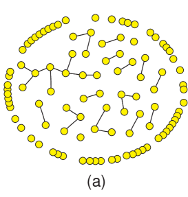
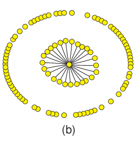
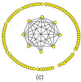
Figure 1: Typical configurations of (a) random, (b) star, and (c) fully-connected networks, generated by simulations performed on a system of $N=100$ nodes and $M=25$ links with $(J_{1},J_{2})=$ (a) $(2,1)$, (b) $(0.5,1)$, and (c) $(2,1)$ at temperature $T=$ (a) $1.36$, (b) $0.12$, and (c) $0.2$.

In view of these, we expect that the system displays a topological phase transition between a random network and one of the two compact networks mentioned above. We first describe the phase transition at the mean-field level, which discloses that the phase transition occurs only at finite system sizes and has strong first-order nature. To confirm this, we carry out numerical simulations and observe discontinuity in energy, hysteresis, and metastability.

3 Mean-field analysis

We begin with the mean-field analysis of the phase transitions between the disordered phase (the random network) and the ordered one (either the fully-connected network or the star network). To describe those transitions, we introduce different order parameters, defined to become $O(1)$ in one configuration and $O(1/M)$ in the other. Expressed as a function of the order parameter and the temperature, the free energy has a maximum between the two extreme configurations due to the entropy contributions at finite temperatures. Comparing the free energies of the two configurations, we determine the low- and the high-temperature phases.

3.1 Phase transition between star and fully-connected networks

We first consider the transition between star (S) and fully-connected (F) networks and probe the phase boundary at which the two phases adjoin. To distinguish the two, we introduce the order parameter measuring the number of nodes having the largest degree,

$$\phi=\frac{n_{k_{max}}}{n}$$ (2)

where it is assumed that among the $n$ non-isolated nodes there exist only two kinds of nodes: $n_{k_{max}}\,(=n\phi)$ nodes of the largest degree (fully connected to each other) and the remaining $n(1-\phi)$ nodes connected only to the former $n_{k_{max}}$ nodes, i.e., having $n\phi$ links. We consider an ensemble of a fixed total number of links, $M$, which are distributed among $n$ non-isolated nodes only. Then $n$ and $\phi$ are related via

$$\frac{n\phi(n\phi-1)}{2}+n\phi n(1-\phi)=M.$$ (3)

In terms of this order parameter, the energy reads approximately

$$E = -\frac{J_{1}}{2M}[(n-1)^{2}n\phi(n\phi-1)+2n(n-1)(n\phi)^{2}(1-\phi)]$$ (4)

$$-\frac{J_{2}}{M}[(n-1)^{2}n\phi+n(n\phi)^{2}(1-\phi)],$$

which reaches the maximum between $\phi=(M+1)^{-1}$ and $\phi\approx 1$ corresponding to a star and a fully-connected network, respectively. We thus compare the energy for the two kinds of network. In the case of a star network, we have $n-1=M$, and

$$E_{S} \equiv E(\phi{=}n^{-1})=-\frac{J_{1}}{M}(n-1)^{2}-\frac{J_{2}}{M}[(n-1)^{2}+(n-1)]$$ (5)

$$= -(J_{1}+J_{2})M-J_{2}.$$

For a fully-connected network, on the other hand, we have $n(n-1)=2M$, and

$$E_{F} \equiv E(\phi{=}1)=-\frac{J_{1}}{M}\frac{n(n-1)^{3}}{2}-\frac{J_{2}}{M}n(n-1)^{2}$$ (6)

$$\approx -2J_{1}M-2J_{2}\sqrt{2M}.$$

Comparison of Eqs. (5) and (6) shows that $E_{F}$ becomes lower than $E_{S}$ for $J_{1}/J_{2}>1-2\sqrt{2/M}+1/M$. It is thus concluded that the ground state corresponds to a fully-connected/star network for $J_{1}$ larger/smaller than $J_{2}$ in the thermodynamic limit ($M\rightarrow\infty$).

We next consider the phase boundary at finite temperatures. To obtain the free energy at finite temperatures, we should take into account the entropy, defined to be $S(\phi)\equiv\ln\Omega_{\phi}$. As a non-isolated node belongs to either a group of $n\phi$ nodes of the largest degree or the other group of remaining nodes, we write the number of distinct accessible configurations in the form

$$\Omega_{\phi}=\left(\begin{array}[]{c}N\\ n\end{array}\right)\left(\begin{array}[]{c}n\\ n\phi\end{array}\right).$$ (7)

The first-order transition between star and fully-connected networks is manifested by the barrier in the free energy $F(\phi)=E-TS$ between two competing minima. As addressed, the transition temperature may be determined by comparing the free energy for the two phases. For a star network, we have $n\phi=1$ and $n=M+1$, thus

$$S_{S}=\ln\left(\begin{array}[]{c}N\\ M+1\end{array}\right)+\ln(M+1)\approx g(\alpha)M,$$ (10)

where $\alpha\equiv 2/\langle k\rangle$ and $g(\alpha)=\ln[\alpha^{\alpha}(\alpha-1)^{1-\alpha}]$. For a fully-connected network, $\phi=1$ and the number of non-isolated nodes is given by $n\approx\sqrt{2M}$, which leads to the entropy

$$S_{F}=\ln\left(\begin{array}[]{c}N\\ \sqrt{2M}\end{array}\right)\approx\sqrt{\frac{M}{2}}\left(\ln M+2\ln\alpha+1-\ln 2\right).$$ (13)

The free energy for each type of network thus reads

$$F_{S} = -(J_{1}+J_{2})M-J_{2}-Tg(\alpha)M$$

$$F_{F} = -2J_{1}M-2J_{2}\sqrt{2M}-T\sqrt{\frac{M}{2}}\left(\ln M+2\ln\alpha+1-\ln 2\right).$$ (14)

The condition $F_{S}=F_{F}$ at $T=T_{c}$ then leads to the transition temperature

$$T_{c}\approx\frac{1}{g(\alpha)}\left[J_{1}-J_{2}\left(1-2\sqrt{\frac{2}{M}}+\frac{1}{M}\right)\right],$$ (15)

below which the system makes a fully-connected network. Note that the transition exists only when $J_{1}>J_{2}$ in the thermodynamic limit. This analysis does not include the true high-temperature phase, which is described by the random network; this is considered in the following section.

3.2 Phase transition between random and fully-connected networks

To examine the phase transition between a random (R) network and a fully-connected one, we define the order parameter $\psi$ to be the average connectivity $k$ of non-isolated nodes relative to the number $n$ of such nodes:

$$\psi=\frac{k}{n},$$ (16)

where the number of total links $M=nk/2$ is constant, thus leading to $\psi=2M/n^{2}$. The order parameter $\psi$ defined above conveniently characterizes the two phases, taking the values $1/M$ and $1-(2M)^{-1/2}$ for the random and fully-connected networks, respectively.

At the mean-field level, the energy reads

$$E\approx-J_{1}k^{2}-\frac{J_{2}}{M}nk^{2}=-2J_{1}M\psi-2J_{2}\sqrt{2M\psi}.$$ (17)

To evaluate the entropic contribution to the free energy at finite temperatures, we write the number of accessible configurations

$$\Omega_{\psi}=\left(\begin{array}[]{c}N\\ n\end{array}\right)\left(\begin{array}[]{c}\frac{1}{2}n(n-1)\\ M\end{array}\right),$$ (18)

with $n=\sqrt{2M/\psi}$. With the help of Stirling’s formula, the entropy is expressed as a function of $\psi$:

$$S=\ln\Omega_{\psi}\approx n+n\ln\left(\frac{N}{n}\right)+M+M\ln\left(\frac{1}{\psi}-1\right),$$ (19)

the first two terms of which are negligible in case $\psi\approx 1/M$.

Figure 2: Free energy $F(\psi)$ versus the order parameter $\psi$, obtained from the mean-field analysis of the system of $N=1000$ nodes and $M=250$ links with $J_{1}=2$ and $J_{2}=1$ at temperature $T=0.2,0.6$, and $1$. At temperature $T$ higher/lower than the transition temperature $T_{c}=0.6$, the free energy of a random network is lower/higher than that of a fully-connected network. At $T=T_{c}$, the two phases coexist and a first-order phase transition takes place between them.

Note that both the energy and the entropy are monotonically decreasing functions of the order parameter $\psi$. As displayed in Fig. 2, the free energy reaches a maximum between $1/M$ and $1-(2M)^{-1/2}$ at finite temperatures. This indicates that the phase transition is again first-order. Taking the leading terms in the entropy, we compute the free energy in the two phases:

$$F_{F} \equiv F(\psi{=}1{-}(2M)^{-1/2})\approx-2J_{1}M-2\sqrt{2M}J_{2}-T\sqrt{2M}(\ln\sqrt{2M}+1)$$

$$F_{R} \equiv F(\psi{=}M^{-1})\approx-2J_{1}-2\sqrt{2}J_{2}-TM(\ln M+1).$$ (20)

At the transition temperature $T_{c}$, the two phases have the same free energy (see Fig. 2). Equating the above two expressions, i.e., $F_{F}(T_{c})=F_{R}(T_{c})$, we obtain the transition temperature

$$T_{c}=\frac{2J_{1}+2\sqrt{2/M}J_{2}}{\ln M+1},$$ (21)

which depends on $J_{1}$ but very weakly on $J_{2}$. In particular, the transition temperature decreases logarithmically with $M$, which indicates that in the thermodynamic limit random networks are prevalent at finite temperatures.

3.3 Phase transition between star and random networks

The phase transition between a star network and a random one is described by the order parameter [1]

$$\Phi=\frac{k_{max}}{M},$$ (22)

where $k_{max}$ is the largest degree of the network. The star-network phase is characterized by a large value of the order parameter, i.e., $\Phi\approx 1$. In terms of this order parameter, the energy function is approximately given by

$$E\approx-J_{1}k_{max}-\frac{J_{2}}{M}k_{max}^{2}=-J_{1}M\Phi-J_{2}M\Phi^{2}$$ (23)

although it does not represent the random network phase well. To estimate roughly the transition temperature $T_{c}$, we consider the number of accessible configurations

$$\Omega_{\Phi}=N\left(\begin{array}[]{c}N-1\\ k_{max}\end{array}\right)\left(\begin{array}[]{c}\frac{1}{2}(N-1)(N-2)\\ M-k_{max}\end{array}\right).$$ (24)

This gives the leading expression of the entropy in terms of the order parameter $\Phi$:

$$S=-\Phi M\ln N$$ (25)

up to an additive constant, as reported in Ref. [1].

Comparing the resulting free energy function in the two phases, namely, at $\Phi=1$ and at $\Phi\approx 0$, we find that the former, corresponding to the star network, provides the global minimum of the free energy at low temperatures. The transition temperature below which the random network turns to a star network is given by

$$T_{c}\approx\frac{J_{1}+J_{2}}{\ln N},$$ (26)

which again decreases logarithmically with the size $N$. It is thus concluded that the phase transition occurs only in a finite system.

4 Numerical results

In this section we present results of Monte Carlo simulations performed for various values of $J_{1}/J_{2}$ and system size $N=100,200,400$, and $1000$. The average connectivity of the whole network is fixed to be $\langle k\rangle=0.5$, so that the number of total links is given by $M=N\langle k\rangle/2=N/4$. First, a random network is generated by connecting randomly selected two nodes $M$ times, then the system is annealed from high temperatures via the standard Metropolis algorithm with randomly selected links rewired. We allow a dangling node to be deprived of its link and expect many isolated nodes to appear at the transition. Typical network configurations obtained thus are shown in Fig. 1.

Figure 3 exhibits the phase diagram of networks constructed by the energy function given by Eq. (1) for $N=200$ and $1000$. It is observed in both numerical and mean-field results that phase boundaries depend on the system size. As predicted in mean-field analysis, the system undergoes a discontinuous topological phase transition from a random network to a compact one such as a star or a fully-connected network as the temperature is lowered. When $J_{1}$ is smaller/greater than $J_{2}$, the ground state is given by the star/fully-connected network. For $J_{1}/J_{2}\gtrsim 1$, in particular, the star-network phase emerges as an intermediate state, so that there occur double transitions as the temperature is lowered. This is more evident for small system size, which is consistent with the mean-field results.

Figure 3: Topological phase diagram on the $(J_{1}/T,J_{2}/T)$ plane for size $N=$(a) $200$ and (b) $1000$. Simulation results, obtained via cooling from a random network, are depicted by symbols, separating regions of random (R), fully-connected (F), and star (S) networks. Dashed lines are merely guides to the eye, and in particular those at low temperatures, i.e., boundaries between F and S regions, are speculative and just represent $J_{1}/J_{2}=1$, which is the minimum value to produce a fully-connected network as the ground state in numerical simulations. Also shown are results from the mean-field analysis, plotted by solid lines.

In the transition from a random to a fully-connected network of large size, it is observed that at the instant of sudden change of topology, the system tends to be trapped in a characteristic multi-star network which consists of two types of node: A few star nodes connected to all nodes and the remaining peripheral nodes connected only to the star nodes identically. Such a multi-star network appears during most of simulations for $J_{1}/J_{2}>1$ and $N=1000$, the largest system size considered here. However, it disappears if more MC steps are performed, especially on a system of smaller size; this indicates the multi-star network to be a metastable state. Although such a metastable state has also been considered in the mean-field analysis, our free energy function does not have any local minimum corresponding to the metastable state.

Shown in Fig. 3 is discrepancy between numerical and mean-field results, which apparently grows with the system size. Here it should be noted that our numerical results have been obtained from cooling simulations. Considering that the phase transition is strongly discontinuous, accompanied with the hysteresis, we expect to obtain a higher transition temperature in heating simulations. With $T_{1}$ and $T_{2}$ denoting the transition temperatures in cooling and heating simulations, respectively, Fig. 3 displays that the annealed transition temperature $T_{1}$ is lower than the mean-field transition temperature $T_{MF}$. In the specific case of the transition from a random network to a fully-connected one, $T_{1}$ in numerical simulations may be estimated as follows: At temperature $T=T_{1}$, we assume that the slope of the free energy vanishes at $\psi=1/M$ (corresponding to the random network phase) and write $0=dF/d\psi|_{\psi=1/M}\approx-2J_{1}M-\sqrt{2}J_{2}M+T_{1}M^{2}$. This leads to the transition temperature in annealing

$$T_{1}=\frac{2J_{1}+\sqrt{2}J_{2}}{M},$$ (27)

which decreases with the size much faster than the mean-field transition temperature. The discrepancy growing with the system size is thus explained. Similarly, at $T=T_{2}$ in heating from a fully-connected network, we write $0=dF/d\psi|_{\psi\approx 1}\approx-2J_{1}M-J_{2}\sqrt{2M}+T_{2}\sqrt{M/2}\ln(\alpha\sqrt{M/2})$, which gives the transition temperature $T_{2}$ increasing with the system size,

$$T_{2}=\frac{4\sqrt{2M}J_{1}+4J_{2}}{\ln M+2\ln\alpha-\ln 2}.$$ (28)

As a result, the hysteresis becomes more evident as the system size is increased in simulations. Therefore, when the system size is sufficiently large, $T_{MF}$ is expected to locate between $T_{1}$ and $T_{2}$.

Figure 4: Hysteresis in the energy versus temperature curves in cooling and heating simulations for $J_{1}/J_{2}=2.5$ and $N=1000$.

We display in Fig. 4 the behavior of the energy for $J_{1}/J_{2}=2.5$ and $N=1000$, as the temperature is lowered (cooling from the random network) or raised (heating from the fully-connected network which is the ground state). Here the hysteresis is manifested. Note, however, that $T_{2}$ obtained numerically is lower than $T_{MF}$, unlike the above conjecture. We presume that this inconsistency results from fluctuations neglected in estimating $T_{2}$. Indeed fluctuations should assist the system to overcome the free energy barrier, thus lowering $T_{2}$ and also suppressing its indefinite increase with the size.

5 Conclusion

We have constructed equilibrium networks by means of a topological energy function which depends quadratically on the node degrees. The topological phase transitions between random, star, and fully-connected networks have been studied both analytically and numerically, through the use of mean-field and simulation methods. It has been observed that the system undergoes discontinuous transitions between the three types of network as the temperature or the interaction strength relative to the node term is varied. Here the transition temperatures in general decrease logarithmically as the system size grows. The quantitative discrepancy between the mean-field and simulation results is attributed to the marked hysteresis associated with the strong first-order nature of the transition.

References

References

- [1] G. Palla, I. Derényi, I. Farkas, and T. Vicsek, Phys. Rev. E 69, 046117 (2004).
- [2] I. Farkas, I. Derényi, G. Palla, and T. Vicsek, Lect. Notes Phys. 650, 163 (2004).
- [3] J. Park and M.E.J. Newman, Phys. Rev. E 70, 066117 (2004).
- [4] M. Baiesi and S.S. Manna, Phys. Rev. E 68, 047103 (2003).
- [5] J. Berg and M. Lässig, Phys. Rev. Lett 89, 228701 (2002).
- [6] V. Colizza, J.R. Banavar, A. Maritan, and A. Rinaldo, Phys. Rev. Lett 92, 198701 (2004).
- [7] R. Ferrier i Cancho and R.V. Solé, in Statistical Mechanics of Complex Networks, Lecture Notes in Physics Vol. 625, edited by R. Pastor-Satorras, M. Rubi, and A. Diaz-Guilera (Springer, Berlin, 2003) pp. 114-126.
- [8] B. Bollobás, Random Graphs (Academic Press, London, 1985).