Relativistic Collisionless Shocks in Unmagnetized Electron-Positron Plasmas

Abstract

It is shown that collisionless shock waves can be driven in unmagnetized electron-positron plasmas by performing a two-dimensional particle-in-cell simulation. At the shock transition region, strong magnetic fields are generated by a Weibel-like instability. The generated magnetic fields are strong enough to deflect the incoming particles from upstream of the shock at a large angle and provide an effective dissipation mechanism for the shock. The structure of the collisionless shock propagates at an almost constant speed. There is no linear wave corresponding to the shock wave and therefore this can be regarded as a kind of “instability-driven” shock wave. The generated magnetic fields rapidly decay in the downstream region. It is also observed that a fraction of the thermalized particles in the downstream region return upstream through the shock transition region. These particles interact with the upstream incoming particles and cause the generation of charge-separated current filaments in the upstream of the shock as well as the electrostatic beam instability. As a result, electric and magnetic fields are generated even upstream of the shock transition region. No efficient acceleration processes of particles were observed in our simulation.

1. Introduction

Collisionless shocks are driven in various situations in astrophysical plasmas. They often accelerate particles and generate nonthermal high-energy particles. Such shocks in supernova remnants are known as the accelerators of nonthermal electrons (e.g., SN1006; Koyama et al., 1995), and are also believed to be the accelerators of cosmic rays with energies up to the knee energy ($\sim 10^{15.5}$ eV). Collisionless shocks also exist in electron-positron plasmas, for example, that in the Crab nebula, and they are considered to generate nonthermal, high-energy electrons and positrons as well.

Recently, it has been suggested from observations that the magnetic fields are amplified or generated around collisionless shocks in several supernova remnants (Vink & Laming, 2003; Bamba et al., 2003; Völk et al., 2005). These magnetic fields may be generated by the high-energy particles accelerated at the shocks (e.g., Bell, 2004). On the other hand, such a generation mechanism can be related to the microphysics of the collisionless shocks themselves. For the generation of magnetic fields in the relativistic shocks associated with the afterglows of gamma-ray bursts, Medvedev & Loeb (1999) suggested that the Weibel instability (Weibel, 1959; Fried, 1959) is driven at the shock and generates strong magnetic fields. This mechanism can work in shocks in electron-positron plasmas as well.

For electron-positron plasmas, the Weibel instability has been investigated in detail by using numerical simulations. Several particle-in-cell simulations showed that in counterstreaming electron-positron plasmas, the Weibel instability develops and generates a strong, sub-equipartition magnetic field (Kazimura et al., 1998; Silva et al., 2003). Furthermore, some authors found that in their simulations with longer calculation times, a shock-like structure that associates with a strong magnetic field is formed even in unmagnetized electron-positron plasmas (Gruzinov, 2001; Haruki & Sakai, 2003). Thus, it should be clarified whether the shock-like structure can be regarded as a shock from a macroscopic point of view, for example, whether the structure dissipates the upstream bulk kinetic energy at the “shock” transition region or propagates at a steady speed into the upstream plasma, etc., as well as other detailed features. If they are considered as shocks, it is also important to elucidate the role of the strong magnetic fields generated by the Weibel-like instability in the dissipation of the shock.

In this study, we further investigate the dynamics of collisionless shocks in unmagnetized electron-positron plasmas in detail by performing a high-resolution two-dimensional particle-in-cell simulation and confirm that a kind of collisionless shocks indeed forms mainly due to the magnetic fields generated by the Weibel-like instability. However, we also find that no efficient particle acceleration occurs in the shock and the generated magnetic fields rapidly decay within the shock transition region, while in the real world, particles are accelerated at the shocks and large-scale, sub-equipartition magnetic fields are generated around the shocks. The reasons why these processes are not observed in our simulation may be related to the background magnetic field, the spatial and temporal scales of the simulation, or the composition of the plasma.

2. Simulation

In order to investigate the collisionless shocks in electron-positron plasmas without background magnetic fields, we performed numerical simulations. The simulation code is a relativistic, electromagnetic, particle-in-cell code with two spatial and three velocity dimensions (2D3V) developed based on a standard method described by Birdsall & Langdon (1991). Thus, the basic equations of the simulation are the Maxwell’s equations (in Gaussian units):

$$\frac{1}{c}\frac{\partial\mathbf{E}}{\partial t}=\nabla\times\mathbf{B}-\frac{4\pi}{c}\mathbf{J},\qquad\frac{1}{c}\frac{\partial\mathbf{B}}{\partial t}=-\nabla\times\mathbf{E},$$ (1)

with

$$\nabla\cdot\mathbf{E}=4\pi\rho,\qquad\nabla\cdot\mathbf{B}=0,$$ (2)

as constraints, where $c$ is the speed of light; $\mathbf{E}$ and $\mathbf{B}$, the electric and magnetic fields, respectively; $\mathbf{J}$, the current density; and $\rho$, the charge density, together with the equation of motion of particles:

$$\frac{d\mathbf{u}}{dt}=\frac{q}{mc}\left(\mathbf{E}+\frac{\mathbf{u}\times\mathbf{B}}{\gamma}\right),$$ (3)

where $q$ and $m$ are the charge and mass of the particle, respectively; $\gamma$, the Lorentz factor of the particle; and $\mathbf{u}\equiv\gamma\mathbf{v}/c$, the 4-velocity of the particle (where $\mathbf{v}$ is the ordinary 3-velocity). Particle velocities are often denoted in terms of the 4-velocity throughout this paper.

In the following, we consider $\tau=\omega_{\mathrm{pe,0}}^{-1}$ as the unit of time and the electron skin depth $l_{0}=c\omega_{\mathrm{pe,0}}^{-1}$ as the unit of length, where $\omega_{\mathrm{pe,0}}\equiv(4\pi n_{e0}e^{2}/m_{e})^{1/2}$ is the electron plasma frequency defined for the mean electron number density $n_{e0}$; $m_{e}$ is the electron mass, and $-e$ is the electron charge. The units of electric and magnetic fields are both taken as $E_{*}=B_{*}=c(4\pi n_{e0}m_{e})^{1/2}$; they are defined so that their corresponding energy densities are both equivalent to the half of the mean electron rest mass energy density.

The simulations were performed on a grid of $N_{x}\times N_{y}=4096\times 512$ with $3.2\times 10^{8}$ particles for each species. The physical size of the simulation box is $L_{x}\times L_{y}=480\times 60$ in the unit of $l_{0}$. Thus, the size of a cell is $(\Delta x,\Delta y)=(0.12,0.12)$ in the same unit. The time step is taken as $\Delta t=0.025$.

Since we consider collisionless shocks in unmagnetized plasmas, the electromagnetic fields were initially set to zero over the entire simulation box. The boundary condition of the electromagnetic field is periodic in each direction.

In this simulation, a collisionless shock wave is driven according to the well-known “injection method.” There are two walls at $x=30$ and $450$. They reflect particles specularly, but let the electromagnetic waves pass through freely; the electromagnetic waves propagating outside the walls ($0<x<30$ and $450<x<480$) are dissipated by means of Ohmic dissipation so that they cannot reach the wall at the other side. Initially, both the electrons and positrons are loaded uniformly in the region between the two walls with a bulk velocity of $u_{x}=2.0$ (thus, the corresponding bulk Lorentz factor is $\Gamma=2.24$). Their thermal velocities were given so that the distribution of each component of the 4-velocity $u_{i}$ ($i=x,y,z$) obeys the Gaussian distribution with a standard deviation of $\sigma_{\mathrm{th}}=0.1$ in the plasma rest frame, or the “fluid” frame. (In effect, this generates the Maxwell distribution.) At the initial stage of the simulation, particles that were located near the right wall (at $x=450$) were reflected by the wall and then interacted with the incoming particles, i.e., the upstream plasma. This interaction causes some instabilities and then a collisionless shock is formed. It should be noted that the frame of the simulation corresponds to the downstream rest frame. Thus, we observed the propagation of the shock from right to the left in the downstream rest frame.

3. Results

The following figures show the quantities at the end of the simulation ($t=233$) otherwise stated.

3.1. Basic Features of Collisionless Shock

Figure 1 shows the electron number density normalized to the initial number density, or the far upstream number density, measured in the downstream rest frame, $n_{e0}$. In this figure, the left-hand side and the right-hand side correspond to upstream and downstream of the shock, respectively. We observe that the number density rapidly increases while crossing the transition region, which extends roughly from $x=350$ to $400$, and then it becomes homogeneous by moving further downstream. The transition region does not have a one-dimensional structure but a two-dimensional filamentary structure with density fluctuations along the $y$ direction. The typical size of the filaments is in the order of several electron skin depths.

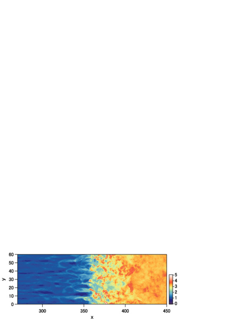
Figure 1.— Electron number density at $t=233$. The value is normalized to the far upstream number density measured in the downstream rest frame (i.e., the simulation frame). The left-hand side and the right-hand side of this figure correspond to upstream and downstream of the shock, respectively. The transition region extends from $x=350$ to $400$.

Figure 2 shows the time development of the electron number density. The horizontal and vertical axes represent the $x$ coordinate and time, respectively. The plotted number density is averaged over the $y$ direction. We observe that the transition region, which is visible as the jump in the number density, propagates upstream, i.e., to the left, with time at an almost constant speed. From this figure, the propagation speed measured in the downstream rest frame is estimated to be $V_{\mathrm{sh,d}}\sim-0.39c$.

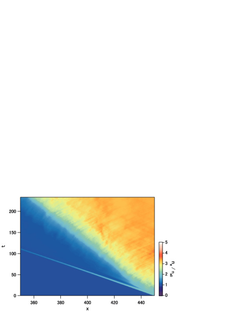
Figure 2.— Time development of the electron number density. The horizontal axis is the $x$ coordinate and the vertical axis is the time. The plotted electron number density is averaged over the $y$ direction. [See the electronic edition of the Journal for a color version of this figure.]

The thin structure propagating upstream at almost the speed of light, which is visible in the lower-left portion of this figure, is due to the particles reflected at the right wall at a very early stage of the simulation. This is of course the consequence of the initial condition, but such a situation may be realized in real cases. Anyway, this structure fades away with time, and it would not affect the structure around the transition region later.

Figure 3 shows the $y$-averaged profiles of three quantities around the shock transition region: (a) the electron number density, $n_{e}/n_{e0}$; (b) the mean velocity of electrons in the $x$-direction, $V_{x}/c$; and (c) the magnitude of electric and magnetic fields, $|E|/E_{*}$ and $|B|/B_{*}$. In Fig. 3a, the solid curve and the dashed curve represent the number densities at $t=233$ and $t=200$, respectively. Comparing the two curves, we see that the transition region propagates upstream keeping its averaged structure almost unchanged. The compression ratio measured in the downstream rest frame is approximately $3.3$. The mean velocity of electrons in the $x$ direction, $V_{x}$, rapidly approaches zero within the transition region (Fig. 3b). In Fig. 3c, it is notable that a strong magnetic field exists within the transition region ($350<x<400$). We also see that behind the shock transition region, the strength of the magnetic field decreases and strong electric and magnetic fields exist even in the upstream region. These points will be mentioned later.

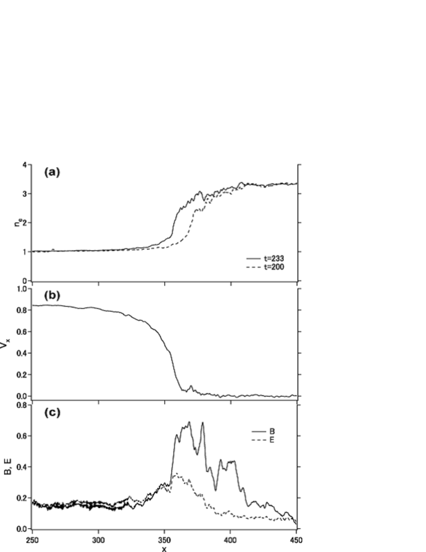
Figure 3.— The $y$-averaged profiles of quantities at $t=233$: (a) the electron number density $n_{e}/n_{e0}$ (solid curve for $t=233$ and dashed curve for $t=200$), (b) the mean velocity in the $x$-direction $V_{x}/c$, and (c) the magnetic field $|B|/B_{*}$ (solid curve) and electric field $|E|/E_{*}$ (dashed curve).

Figure 4a shows the $z$ component of the magnetic field, $B_{z}$. It is clear that a strong magnetic field exists within the transition region ($350<x<400$), as indicated in Fig. 3c. Figure 4b shows the current density in the $x$ direction, $J_{x}$. We observed that there are considerable number of current filaments that carry currents in the $x$ direction within the transition region. The filamentary structure observed in the number density (Fig. 1) is in fact due to the existence of these current filaments. They generate a magnetic field fluctuating in the $y$ direction, as shown in Fig. 4a. This situation in which strong magnetic fields fluctuating perpendicular to the direction of streaming are generated is similar to those in the simulations of the Weibel instability in counterstreaming plasmas (Kazimura et al., 1998; Silva et al., 2003). Therefore, it is reasonable to consider that in the transition region in which the upstream plasma is mixed up with the downstream plasma, a large velocity dispersion in the $x$ direction and hence a large anisotropy in the particle velocity distribution are induced; further, the anisotropy drives the Weibel-type instability, which generates the magnetic field. The typical magnitude of the magnetic field in this region is $|B|\sim 0.7B_{*}$ and the corresponding Larmor radius for the incoming upstream particles with $u=2.0$ is $r_{g}\sim 2.9$, which is comparable to the size of the magnetic field structure, i.e., the current filaments, in the transition region. Therefore, the incoming upstream particles should be isotropised in this region because they are deflected at a large angle by the strong magnetic field at this location. This isotropisation provides an effective dissipation mechanism for the upstream bulk kinetic energy.

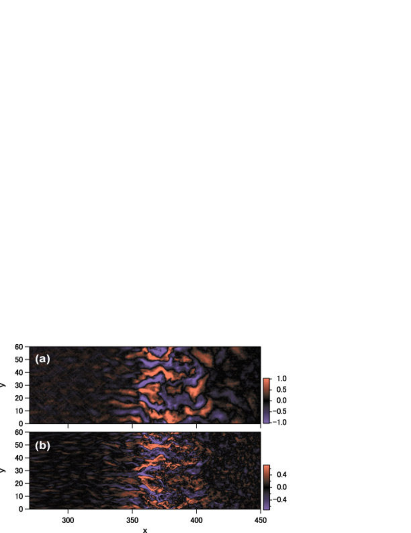
Figure 4.— (a) The $z$ component of the magnetic fields $B_{z}$ and (b) the $x$ component of the current density $J_{x}$ at $t=233$.

Figure 5 shows the $y$-averaged profile of the magnetic energy density normalized by the upstream bulk kinetic energy density. We see that the magnetic energy density reaches about 10% of the upstream bulk kinetic energy density at the peak and decays downstream of the shock. The saturation and decay mechanism of the magnetic field would be similar to those of the Weibel instability (Kato, 2005). The current and the magnetic field generated by the instability in each filament saturates when the magnetic field becomes strong enough to deflect the current-carrying particles in the filament. This predicts the sub-equipartition magnetic field at saturation and it is consistent with the simulation result. After the saturation, the current filaments will coalesce with each other to form larger filaments with the decreasing magnetic field strength. We observe the evolution of the structure to a larger scale together with the decay of the magnetic field strength downstream of the shock transition region in Figs. 4a, 3c, and 5.

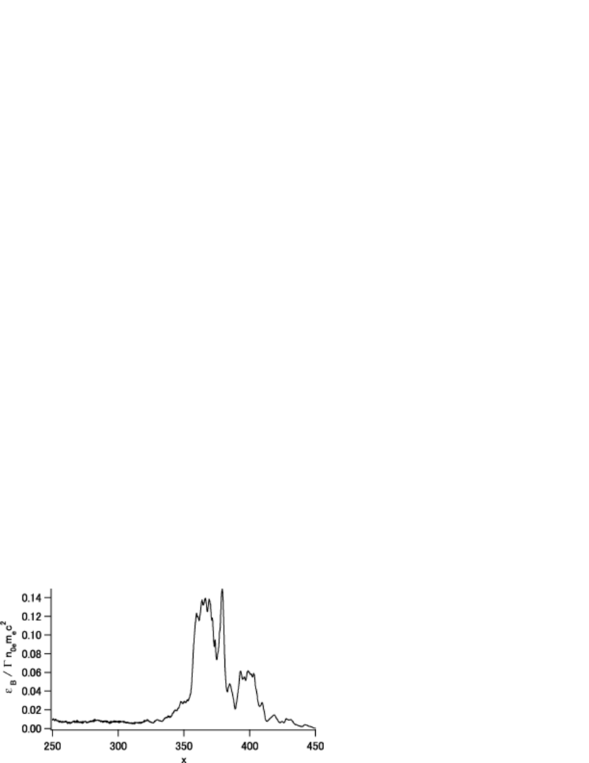
Figure 5.— The $y$-averaged profile of the magnetic energy density normalized by the upstream bulk kinetic energy density at $t=233$, $\epsilon_{B}/\Gamma n_{e0}m_{e}c^{2}$. The magnetic field strength reaches a sub-equipartition level at the peak and rapidly decays in the downstream region.

Figure 6 shows (a) the fluid velocity of electrons in the $x$-direction, $V_{x}/c$, and (b) the mean kinetic energy of the electrons measured in the local fluid rest frame of the electrons expressed in terms of electron rest mass, $\langle\gamma-1\rangle_{\mathrm{fluid}}$. It is evident that the incoming plasma from upstream is rapidly decelerated within the transition region, where the strong magnetic field exists (see also Fig. 4a), and its bulk kinetic energy is converted into random or “thermal” kinetic energy in the downstream rest frame.

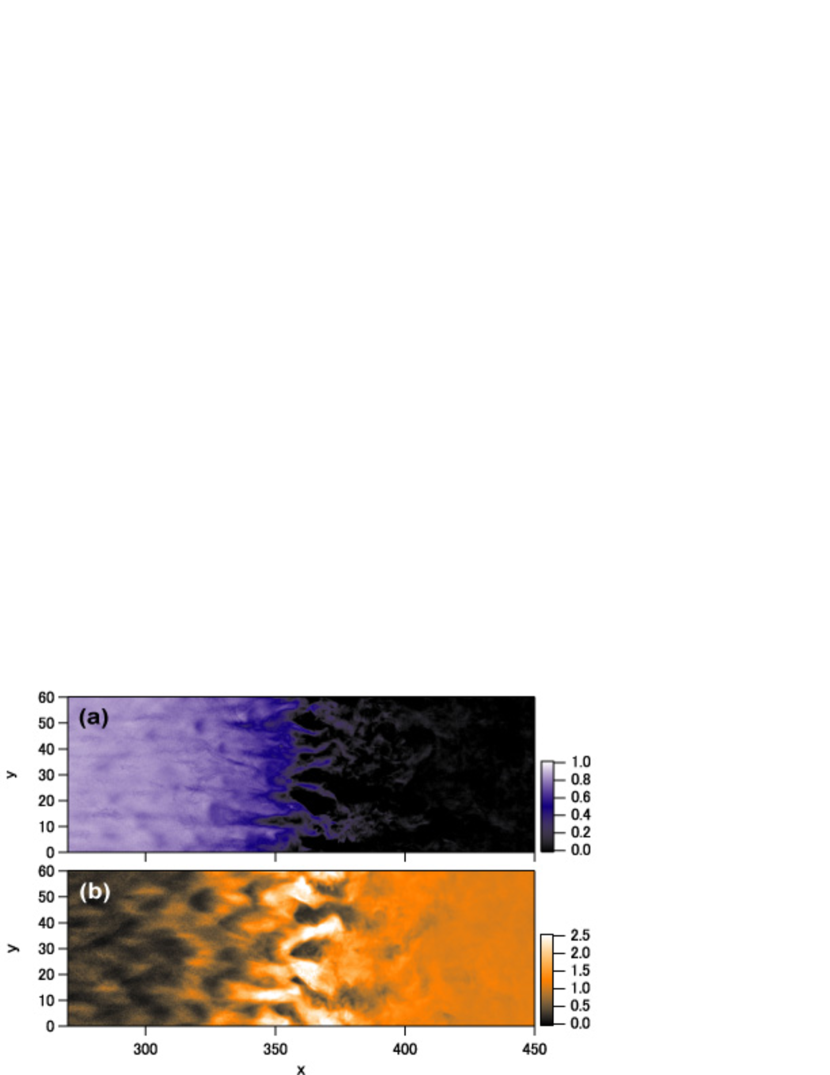
Figure 6.— (a) The $x$ component of the electron mean velocity $V_{x}/c$ and (b) the mean kinetic energy of the electrons measured in the local plasma rest frame of the electrons, $\langle\gamma-1\rangle_{\mathrm{fluid}}$, at $t=233$. It is evident that the bulk kinetic energy of the upstream plasma is converted into the internal kinetic energy within the transition region. [See the electronic edition of the Journal for a color version of this figure.]

Figure 7 shows the standard deviations of (a) $u_{x}$ of electrons, $\sigma_{x}$, and (b) $u_{y}$ of electrons, $\sigma_{y}$, both measured in the local plasma rest frame of the electrons. We observe that the particles are isotropised in the transition region due to the strong magnetic field existing there. It should be noted that, in this two-dimensional simulation, particles are isotropised only on the $x-y$ plane and not in the $z$ direction (c.f. Haruki & Sakai, 2003) because only the Weibel modes with wave vectors on the $x-y$ plane can develop and hence only $B_{z}$ is generated. In a three-dimensional simulation, the Weibel modes with wave vectors in the $z$ direction should develop equally and particles are isotropised in all directions.

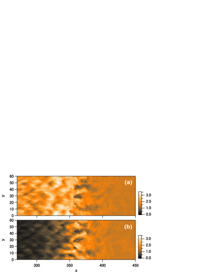
Figure 7.— Standard deviation of (a) $u_{x}$ and (b) $u_{y}$ of electrons both measured in the local plasma rest frame of the electrons. The electrons are isotropised when they pass through the transition region. [See the electronic edition of the Journal for a color version of this figure.]

In a macroscopic view, the features shown in the above figures would be observed as those of shock waves; the shock waves dissipate the upstream bulk kinetic energy in the shock transition region and propagate at an almost constant speed into the upstream plasma. In this sense, we can regard this as a collisionless shock. In this shock, the magnetic field in the transition region generated by the Weibel-like instability plays an essential role in the dissipation process of the collisionless shock in unmagnetized plasmas. It should be noted that the shock has no corresponding fundamental linear wave, which is required to define the Mach number, in contrast to, for example, the perpendicular shocks in magnetized plasmas, in which the magnetosonic wave is the fundamental linear wave of the shock. This point is clear from the fact that the wave vector of the magnetic field in the transition region is in the $y$ direction and not in the $x$ direction or the shock normal in the present case and hence it has an essentially a two-dimensional structure. Thus, it can be said that this is a class of “instability-driven” shock waves. For such shocks, the concept of the Mach number would not be applicable, and the propagation speed of the shock and the width of the transition region would be essentially determined by the nature of the instability that provides the dissipation mechanism at the shock transition region.

3.2. Charge-separated Current Filaments and Backward Flowing Particles

From Fig. 4b, we observe that there are current filaments even in the upstream region ($x<350$). Figure 8a shows the charge density $\rho$. Comparing these two figures, it is evident that these filaments have a net space charge. Since in each filament, $J_{x}$ and $\rho$ have the same sign, these filaments are mainly composed of the incoming upstream particles with $u_{x}>0$. Figure 8b shows the $y$ component of the electric field, $E_{y}$. We observe that $E_{y}$ is generated between these filaments due to their space charge. As shown in Fig. 4a, these filaments also generate magnetic field $B_{z}$ around them. Thus, rather strong electric and magnetic fields exist in the upstream region, as shown in Fig. 3c. Figure 8c shows the $x$ component of the electric field. We observed that strong electric fields exist at the upstream edge of the transition region and that there is a coherent structure in $E_{x}$ in the upstream of the transition region ($x<350$).

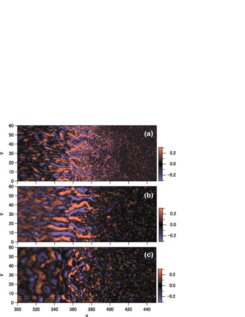
Figure 8.— (a) Charge density $\rho$, (b) the $y$ component of the electric field $E_{y}$ and (c) the $x$ component of the electric field $E_{x}$ at $t=233$.

The region where the charge-separated current filaments exist would correspond to “the charge separation layer” suggested by Milosavljević et al. (2006). As they pointed out, these filaments need a small fraction of the particles flowing backward to stabilize themselves. Figure 9 shows the $x-u_{x}$ phase-space plot of electrons at $t=233$. We observe that the particles flowing backward ($u_{x}<0$) are supplied around the shock transition region ($x\sim 350$). These particles would stabilize the charge-separated current filaments in the charge separation layer. They can also drive the electrostatic beam instability. The coherent electrostatic field $E_{x}$ upstream of the transition region ($x<350$; see Fig. 8c) would be induced by this instability. These particles should also contribute to drive the Weibel-type instability around the transition region.

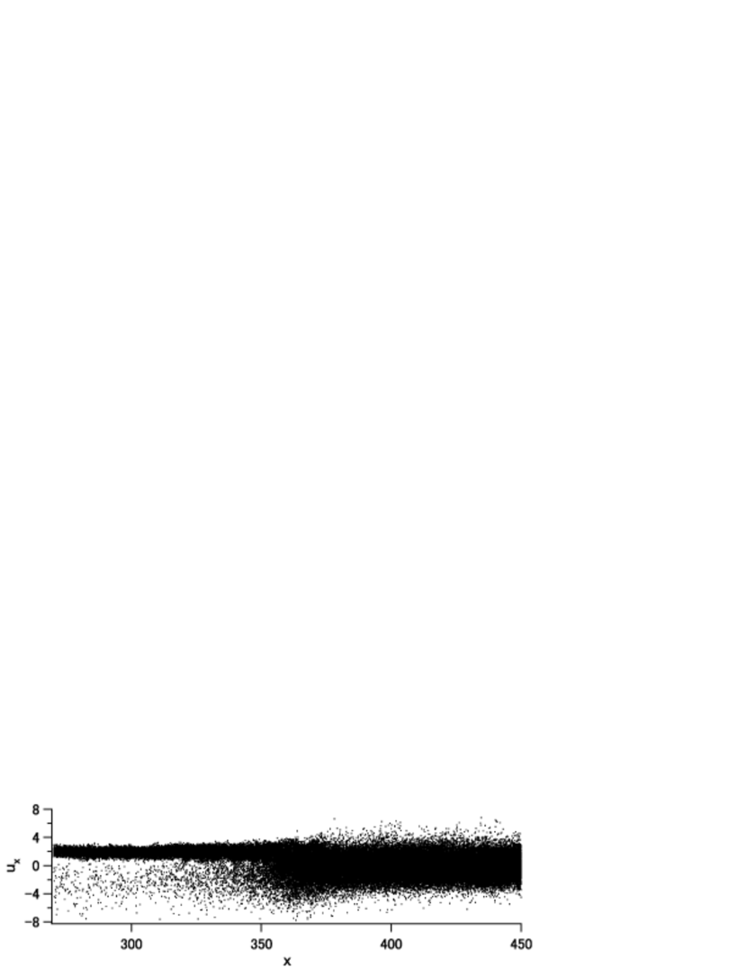
Figure 9.— The $x-u_{x}$ phase-space plot of electrons at $t=233$. Upstream of the shock transition region ($x<350$), a fraction of particles flow backward, which causes two-stream type instabilities. In the downstream region ($x>370$), electrons are thermalized (along the $x$ direction).

Figure 10 shows the time development of the number density of electrons again as in Fig. 2, but with contours. We observe that there is a “precursor” region in which the number density is within a range of $1.1<n_{e}/n_{e0}<1.9$ in front of the transition region. In this region, the increase in the number density from that in the upstream plasma $n_{e0}$ would be mainly due to the electrons flowing backward (see also Fig. 9). The width of the precursor region is almost constant ($\Delta x\sim 30$) after $t\sim 100$.

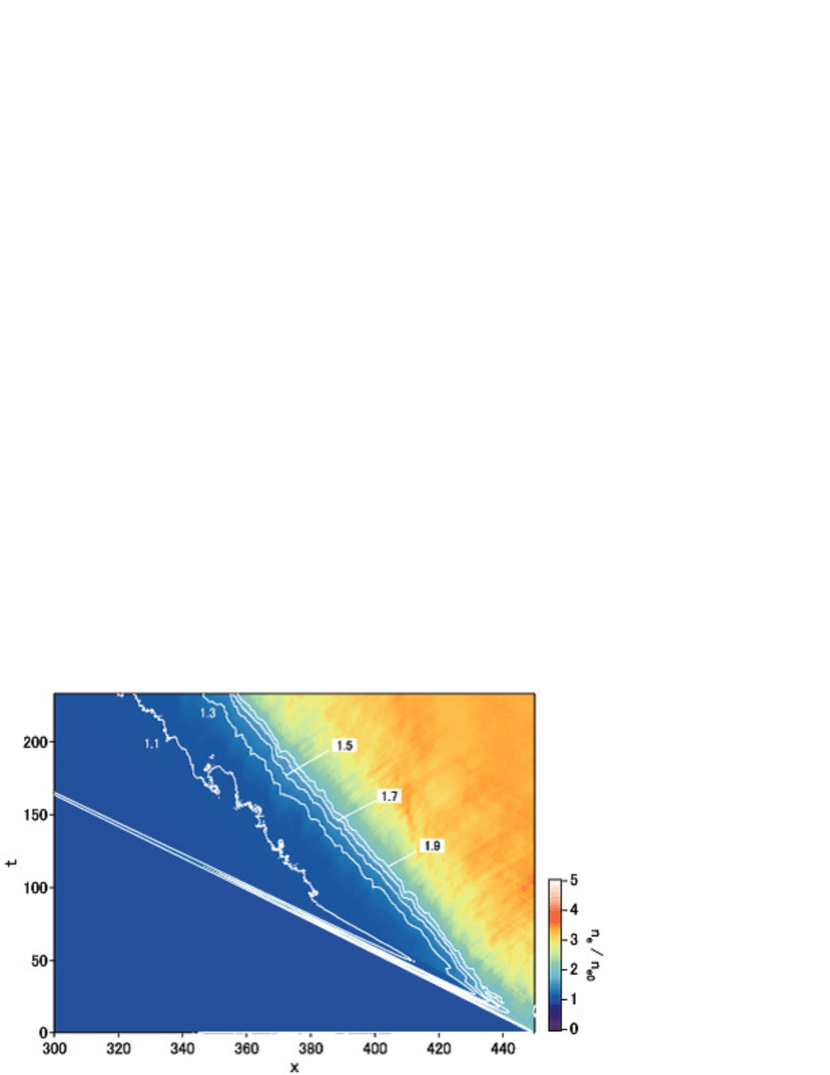
Figure 10.— Time development of the electron number density as in Fig. 2, but with contours. The width of the precursor region ($1.1<n_{e}/n_{e0}<1.9$), where the density of the electrons flowing backward is high, is almost constant ($\Delta x\sim 30$) after $t\sim 100$. [See the electronic edition of the Journal for a color version of this figure.]

As already shown in Fig. 4b, there are current filaments in the transition region. However, they are charge-separated only at the filament edges except those at the downstream side that are continuously connected to the thermalized downstream region (see Fig. 8a). The strength of the magnetic and electric fields, current density, and charge density all attain their maximum values in this region, and the upstream kinetic energy is dissipated mainly by the magnetic field and partly by the electric field.

A fraction of the downstream particles flowing backward with $u_{x}<u_{\mathrm{sh,d}}\sim-0.42$, which is the 4-velocity corresponding to $V_{\mathrm{sh,d}}$, can return upstream through the filaments that carry the currents in the same direction as the particles. On the other hand, if the particles return through the filament carrying opposite currents, the magnetic fields in the filaments repel the particles from the filaments. Figure 11 shows the distribution of electrons that are flowing upstream with $u_{x}<-2$. By comparing with $J_{x}$ in Fig. 4b, we observed that these electrons indeed flow in the current filaments with $J_{x}>0$. In a similar manner, the positrons flow backward in the current filaments, but with $J_{x}<0$ (not shown here). However, only a small fraction of the backward flowing particles can move to the upstream region ($x<350$) because large potential barriers exist, caused by the charge density at the upstream edge of the filaments (see also Figs. 8a and 8c). The particles that could pass through to the upstream region would contribute to stabilize the charge-separated current filaments in the charge separation layer, as mentioned earlier.

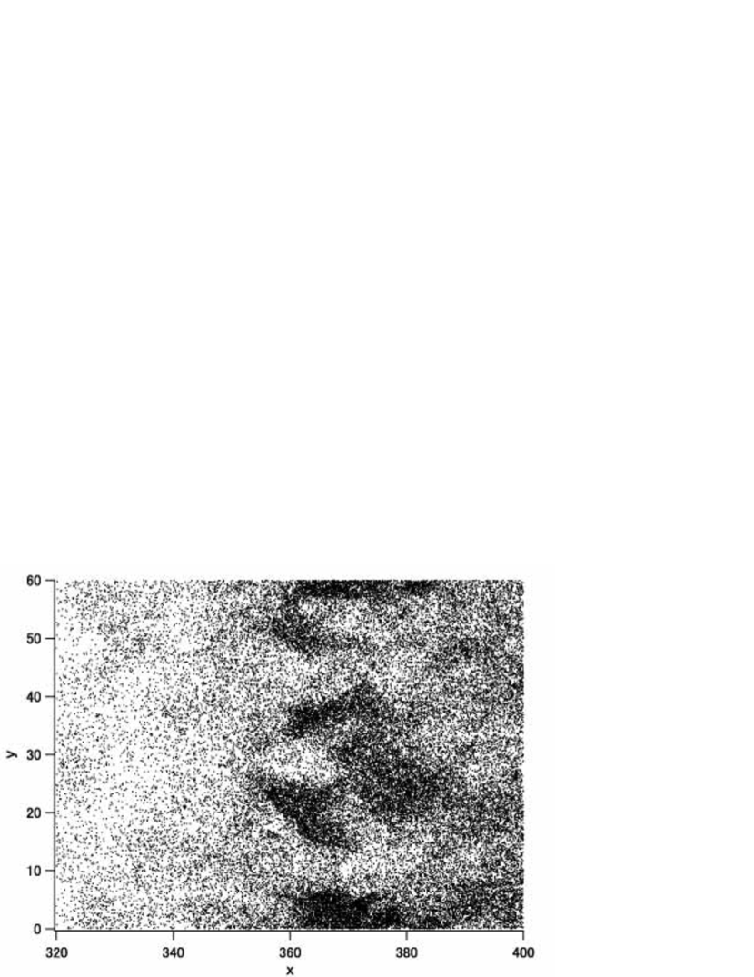
Figure 11.— Distribution of backward flowing electrons with $u_{x}<-2$. They move upstream through the current filaments with $J_{x}>0$. This is evident for $x>350$.

3.3. Particle Energy Distribution and Acceleration

Figure 12 shows the energy histogram of the electrons accumulated over the area between $x=430$ and $x=442$ in the downstream region (the solid histogram). The dashed curve and the dot-dashed curve represent the Maxwell distributions in three and two dimensions, which are defined by

$$N_{3D}(\gamma)=n_{d}\frac{\theta^{2}\gamma(\gamma^{2}-1)^{1/2}}{2K_{1}(\theta)+\theta K_{0}(\theta)}\exp(-\gamma\theta),$$ (4)

and

$$N_{2D}(\gamma)=n_{d}\frac{\theta^{2}\gamma}{\theta+1}\exp\left[-(\gamma-1)\theta\right],$$ (5)

respectively. Here, $n_{d}$ is the number density in the downstream region, $K_{i}$ is the modified Bessel function of the second kind (Abramowitz & Stegun, 1965), and $\theta$ is determined so that $\int_{1}^{\infty}\gamma N(\gamma)d\gamma=\langle\gamma\rangle\sim\sqrt{5}$, which is expected if the upstream bulk kinetic energy is completely converted into the internal kinetic energy in the downstream rest frame. From Fig. 3a, we consider $n_{d}\sim 3.3\ n_{e0}$. It is observed that the electron distribution fits neither of the Maxwell distributions.

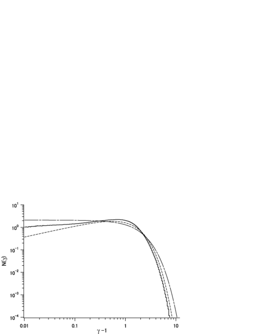
Figure 12.— Histogram of the kinetic energy of the downstream electrons within $430<x<442$ at $t=233$ (solid line). The horizontal axis is the kinetic energy normalized by the electron rest mass energy, $\gamma-1$. The dashed curve and the dot-dashed curve represent the Maxwell distribution for three and two dimensions, respectively.

Figure 13 shows the energy histogram of all electrons in the simulation box by a solid histogram. For reference, we plotted the three-dimensional Maxwell distribution by the dotted curve. Their normalizations are arbitrary, and there is no significant particle acceleration.

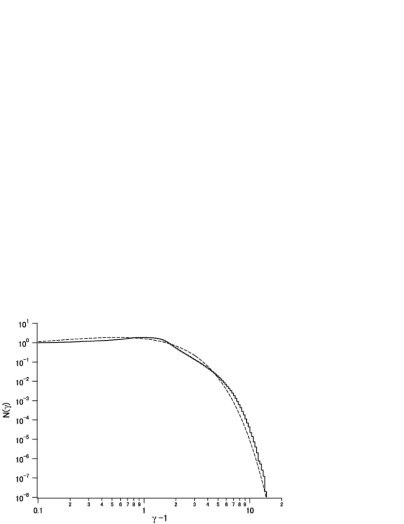
Figure 13.— Histogram of the kinetic energy of all the electrons in the simulation box (solid line). The three-dimensional Maxwell distribution is also plotted as a reference (dashed curve). There is no significant particle acceleration.

4. Conclusions

The simulation results clearly show that collisionless shocks can be driven in unmagnetized electron-positron plasmas. The structure of the collisionless shock propagates at an almost constant speed. The dissipation of the upstream bulk kinetic energy is mainly due to the deflection of particles by the strong magnetic field generated around the shock transition region by the Weibel-type instability. It is remarkable that this shock has no corresponding linear wave and therefore it can be regarded as a kind of “instability-driven” shock wave. We also observed the electric and magnetic field generation even in the upstream of the shock transition region due to the charge-separated current filaments together with the electrostatic beam instability. We found that a fraction of the downstream thermalized particles return upstream through the shock transition region. These particles would interact with the upstream incoming plasma and cause the generation of the charge-separated current filaments as well as the electrostatic beam instability upstream of the transition region. We did not observe any efficient particle acceleration processes in our simulation, whereas we observed relatively rapid decay of the generated magnetic field within the shock transition region. On the other hand, in the real world, there are many evidences to suggest that particles are accelerated at shocks, and there are several indications that large-scale, sub-equipartition magnetic fields may be generated around these shocks. The reasons why these processes were not observed in our simulation may be that (1) the background magnetic field is essential for them, (2) the spatial and temporal scales of the simulation are too small to deal with them, or (3) these processes are inefficient in the electron-positron shocks.

References

- Abramowitz & Stegun (1965) Abramowitz, M., & Stegun, I.A. 1965, Handbook of Mathematical Functions (New York: Dover).
- Bamba et al. (2003) Bamba, A., Yamazaki, R., Ueno, M., & Koyama, K. 2003, ApJ, 589, 827
- Bell (2004) Bell, A. R. 2004, MNRAS, 353, 550
- Birdsall & Langdon (1991) Birdsall, C. K., & Langdon, A. B. 1991, Plasma Physics via Computer Simulation (IOP Publishing: Bristol).
- Fried (1959) Fried, B. D. 1959, Phys. Fluids, 2, 337
- Gruzinov (2001) Gruzinov, A. 2001, preprint (astro-ph/0111321)
- Haruki & Sakai (2003) Haruki, T., & Sakai, J. 2003, Phys. Plasmas, 10, 392
- Kato (2005) Kato, T. N. 2005, Phys. Plasmas, 12, 080705
- Kazimura et al. (1998) Kazimura, Y., Sakai, J. I., Neubert, T., & Bulanov, S. V. 1998, ApJ, 498, L183
- Koyama et al. (1995) Koyama, K., Petre, R., Gotthelf, E. V., Hwang, U., Matsuura, M., Ozaki, M., & Holt, S. S. 1995, Nature, 378, 255
- Medvedev & Loeb (1999) Medvedev, M. V., & Loeb, A. 1999, ApJ, 526, 697
- Milosavljević et al. (2006) Milosavljević, M., Nakar. E., & Spitkovsky., A. 2006, ApJ, 637, 765
- Silva et al. (2003) Silva, L. O., Fonseca, R. A., Tonge, J. W., Dawson, J. M., Mori, W. B., & Medvedev, M. V. 2003 ApJ, 596, L121
- Vink & Laming (2003) Vink, J., & Laming, J. M. 2003, ApJ, 584, 758
- Völk et al. (2005) Völk, H. J., Berezhko, E. G., & Ksenofontov, L. T. 2005, A&A, 433, 229
- Weibel (1959) Weibel, E. S. 1959, Phys. Rev. Lett., 2, 83