Sphere Lower Bound for Rotated Lattice Constellations in Fading Channels

Abstract

We study the error probability performance of rotated lattice constellations in frequency-flat Nakagami-$m$ block-fading channels. In particular, we use the sphere lower bound on the underlying infinite lattice as a performance benchmark. We show that the sphere lower bound has full diversity. We observe that optimally rotated lattices with largest known minimum product distance perform very close to the lower bound, while the ensemble of random rotations is shown to lack diversity and perform far from it.

I Introduction

In this letter, we study the family of full rate multidimensional signal constellations carved from lattices in frequency-flat Nakagami-$m$ fading channels with $N$ degrees of freedom. In particular, we consider the uncoded case, i.e., no time redundancy is added to the transmitted signal. Current best constellations are designed to achieve full diversity and maximize the minimum product distance [1, 2, 3]. To date, there exists no benchmark to compare the performance of rotated lattice constellations. Recent work ([4]) gives an approximation to the error probability of multidimensional constellations in fading channels, which is not tight and does not always have full diversity.

In this letter, we use the sphere lower bound (SLB), as a benchmark for the performance of such uncoded lattice constellations. The SLB dates back to Shannon’s work [6], and gives a lower bound to the error probability of spherical codes with a given length in the additive white Gaussian noise (AWGN) channel. The application of the SLB to infinite lattices and lattice codes was studied in [7, 8] for the AWGN channel. This SLB yields a lower bound to the error probability of infinite lattices regardless of the lattice structure. An approximated SLB was derived in [9] for spherical codes over the Rayleigh fading channel. Fozunbal et al. [10] extended the SLB to coded communication over the multiple-antenna block-fading channel. A remarkable result of [10] is that, for a fixed number of antennas and blocks, as the code length grows, the SLB converges to the outage probability of the channel with Gaussian inputs [11]. Unfortunately, the outage probability [11, 12] and the SLB of [10] are very far from the actual error probability of uncoded multidimensional constellations. Moreover, as the block length increases, the performance of uncoded modulations degrades, and therefore, the outage probability and the SLB of [10] are not very useful as performance benchmarks.

In this letter, we use the SLB of the infinite lattice as a benchmark for comparing multidimensional constellations in the block-fading channel. We first show that the SLB of infinite lattice rotations for the block fading channel has full diversity regardless of the block length. We illustrate that as the block length increases, the SLB increases as well. We also show that multidimensional constellations obtained by algebraic rotations with largest minimum product distance obtained from pairwise error probability criteria [1, 2, 3] perform very close to the lower bound and that the ensemble of random rotations does not achieve full diversity.

II System model

We consider a flat fading channel whose discrete-time received signal vector is given by

$${\bf y}_{\ell}={\bf H}{\bf x}_{\ell}+{\bf z}_{\ell},\;\;\;\ell=1,\cdots,L$$ (1)

where ${\bf y}_{\ell}\in{\mathbb{R}}^{N}$ is the $N$-dimensional real received signal vector, ${\bf x}_{\ell}\in{\mathbb{R}}^{N}$ is the $N$-dimensional real transmitted signal vector, ${\bf H}=\mathop{\rm diag}\nolimits({\bf h})\in{\mathbb{R}}^{N\times N}$, with ${\bf h}=(h_{1},\dotsc,h_{N})\in{\mathbb{R}}^{N}$, is the flat fading diagonal matrix, and ${\bf z}\in{\mathbb{R}}^{N}$ is the noise vector whose samples are i.i.d. $\sim{\cal N}(0,\sigma^{2})$ with pdf

$$p({\bf z})=(2\pi\sigma^{2})^{-\frac{N}{2}}\exp\left(-\frac{\|{\bf z}\|^{2}}{2\sigma^{2}}\right)$$

We define the signal-to-noise ratio (SNR) as $\rho=1/\sigma^{2}$. A frame is composed of $L$, $N$-dimensional modulation symbols or of $NL$ channel uses. The case of complex signals obtained from $2$ orthogonal real signals can be similarly modeled by (1) by replacing $L$ with $L^{\prime}=2L$.

We assume that the fading matrix ${\bf H}$ is constant during one frame and it changes independently from frame to frame. This corresponds to the block-fading channel with $N$ blocks [12]. We further assume perfect channel state information (CSI) at the receiver, i.e., the receiver perfectly knows the fading coefficients. Therefore, for a given fading realization, the channel transition probabilities are given by

$$p({\bf y}|{\bf x},{\bf H})=(2\pi\sigma^{2})^{-\frac{N}{2}}\exp\left(-\frac{1}{2\sigma^{2}}\|{\bf y}-{\bf H}{\bf x}\|^{2}\right)$$

Moreover, we assume that the real fading coefficients follow a Nakagami-$m$ distribution

$$p_{h}(x)=\frac{2m^{m}x^{2m-1}}{\Gamma(m)}e^{-mx^{2}}$$

where $m>0$ and

$$\Gamma(x)\stackrel{{\scriptstyle\Delta}}{{=}}\int_{0}^{+\infty}t^{x-1}e^{-t}dt$$

is the Gamma function [14]. We define the coefficients $\gamma_{n}=h_{n}^{2}$ for $n=1,\dotsc,N$, which correspond to the fading power gains with pdf

$$p_{\gamma}(x)=\frac{m^{m}x^{m-1}}{\Gamma(m)}e^{-mx}$$

and cdf

$$P_{\gamma}(x)=1-\overline{\Gamma}(mx,m),$$

respectively, where

$$\overline{\Gamma}(a,x)\stackrel{{\scriptstyle\Delta}}{{=}}\frac{1}{\Gamma(a)}\int_{x}^{+\infty}t^{a-1}e^{-t}dt$$

is the normalized incomplete Gamma function [14]. By analyzing Nakagami-$m$ fading, we can recover the analysis for a large class of fading statistics, including Rayleigh fading by setting $m=1$ and Rician fading with parameter $K$ by setting $m=(K+1)^{2}/(2K+1)$ [15].

II-A Multidimensional Lattice Constellations

We assume that the transmitted signal vectors ${\bf x}$ belong to an $N$-dimensional signal constellation ${\cal S}\subseteq{\mathbb{R}}^{N}$. We consider signal constellations ${\cal S}$ that are generated as a finite subset of points carved from the infinite lattice $\Lambda=\{{\bf M}{\bf u}:{\bf u}\in{\mathbb{Z}}^{N}\}$ with full rank generator matrix ${\bf M}\in{\mathbb{R}}^{N\times N}$ [5]. For normalization purposes we fix $\det({\bf M})=1$. For a given channel realization, we define the faded lattice seen by the receiver as the lattice $\Lambda^{\prime}=\{{\bf M}^{\prime}{\bf u}:{\bf u}\in{\mathbb{Z}}^{N}\}$, whose generator matrix is given by ${\bf M}^{\prime}={\bf H}{\bf M}$.

In order to simplify the labeling operation, constellations are of the type ${\cal S}=\{{\bf M}{\bf u}+{\bf x}_{0}:{\bf u}\in{\mathbb{Z}}_{M}^{N}\}$, where ${\mathbb{Z}}_{M}=\{0,1,\dotsc,M-1\}$ represents an integer PAM constellation, $\log_{2}(M)$ is the number of bits per dimension and ${\bf x}_{0}$ is an offset vector which minimizes the average transmitted energy. Therefore, the rate of such constellations is $R=\log_{2}M$ bit/s/Hz. This is usually referred to as full-rate uncoded transmission.

In order to avoid shaping loss it is convenient to use cubic lattice constellations [1, 2]. This implies that ${\bf M}$ should be an orthogonal matrix (${\bf M}{\bf M}^{T}={\bf I}$) . Nevertheless, this is not required in the calculation of the SLB.

II-B Maximum Likelihood Decoding Error Probability

At a given $\ell$, a maximum likelihood (ML) decoder with perfect CSI makes an error whenever

$$\|{\bf y}_{\ell}-{\bf H}{\bf w}\|^{2}\leq\|{\bf y}_{\ell}-{\bf H}{\bf x}\|^{2}$$

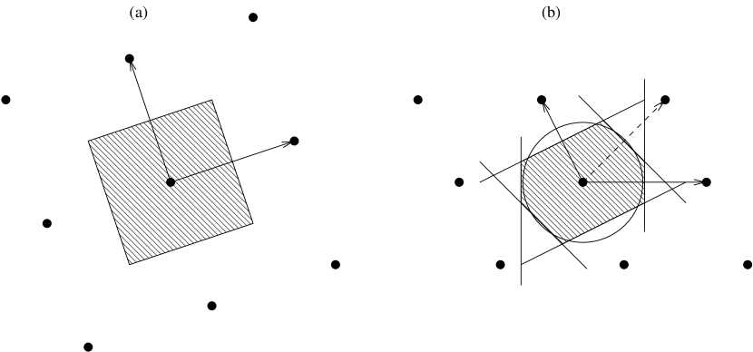
Figure 1: The decision regions of the rotated ${\mathbb{Z}}^{2}$ lattice: (a) before fading, (b) after fading ${\bf h}=(1,0.5)$.

for some ${\bf w}\in{\cal S},\,\,{\bf w}\neq{\bf x}$. These inequalities define the so called decision region around ${\bf x}$ (see Figure 1). Under ML decoding, the frame error probability is then given by

$$P_{\rm f}(\rho)={\mathbb{E}}[P_{\rm f}(\rho|{\bf h})]={\mathbb{E}}\left[1-(1-P_{\rm s}(\rho|{\bf h}))^{L}\right]$$ (2)

where $P_{\rm f}(\rho|{\bf h})$ and $P_{\rm s}(\rho|{\bf h})$ are the frame and $N$-dimensional symbol error probabilities for a given channel realization and SNR $\rho$, where the average is taken over the fading distribution. For a given constellation ${\cal S}$, we can write that

$$P_{\rm s}(\rho|{\bf h})={\mathbb{E}}[P_{\rm s}(\rho|{\bf x},{\bf h})]=\frac{1}{|{\cal S}|}\sum_{{\bf x}\in{\cal S}}\int_{{\bf y}\notin{\cal V}({\bf x},{\bf h})}\!\!p({\bf y}|{\bf x},{\bf h})d{\bf y}$$

where ${\cal V}({\bf x},{\bf h})$ is the decision region or Voronoi region for a given multidimensional lattice constellation point ${\bf x}$ and fading ${\bf H}$. Computing the regions ${\cal V}({\bf x},{\bf h})$ and the exact error probability is in general a very hard problem. In this paper we use the SLB [6] as a lower bound on $P_{\rm f}$. We define the diversity order as the asymptotic (for large SNR) slope of $P_{\rm f}$ in a log-log scale,

$$d=-\lim_{\rho\to\infty}\frac{\log P_{\rm f}(\rho)}{\log\rho}.$$ (3)

The diversity order is usually a function of the fading distribution and the signal constellation ${\cal S}$. In this paper, we show that the diversity order is the product of the signal constellation diversity and a parameter of the fading distribution. In particular, we say that a constellation ${\cal S}$ has full diversity if the ML decoder is able to decode correctly in presence of $N-1$ deep fades.

III Sphere Lower Bound of a Faded Lattice

In this Section, we recall the basics of the SLB for infinite lattices ${\cal S}=\Lambda$ [7, 8] and we apply it to bound $P_{\rm f}(\rho)$. The first simplification stems from the geometrical uniformity of lattices, which implies that [7, 8]

$${\cal V}({\bf x},{\bf h})={\cal V}({\bf w},{\bf h}),~{}~{}\forall{\bf x},{\bf w}\in\Lambda,{\bf x}\neq{\bf w}$$

namely, for a given fading realization, the Voronoi regions of all lattice points are equal. Let ${\cal V}_{\Lambda}({\bf h})$ denote such Voronoi region of the faded lattice. Therefore, and without loss of generality, we safely assume the transmission of the all-zero codeword, i.e., ${\bf x}_{\ell}={\bf 0}~{},~{}\ell=1,\dotsc,L$. Then, the error probability is given by [5]

$$P_{\rm f}(\rho)=1-{\mathbb{E}}\left[\left(1-\int_{{\bf z}\notin{\cal V}_{\Lambda}({\bf h})}p({\bf z})d{\bf z}\right)^{L}\right].$$ (4)

Due to the circular symmetry of the Gaussian noise, replacing ${\cal V}_{\Lambda}({\bf h})$ by an $N$-dimensional sphere ${\cal B}({\bf h})$ of the same volume and radius $R({\bf h})$ [6], yields the corresponding SLB on the lattice performance [7, 8]

$$P_{\rm f}(\rho)\geq P_{\rm slb}(\rho)\stackrel{{\scriptstyle\Delta}}{{=}}1-{\mathbb{E}}\left[\left(1-\int_{{\bf z}\notin{\cal B}({\bf h})}p({\bf z})d{\bf z}\right)^{L}\right]$$ (5)

Since the volume of ${\cal B}({\bf h})$ is [5]

$$\mathop{\rm vol}\nolimits({\cal B}({\bf h}))=\frac{\pi^{\frac{N}{2}}R({\bf h})^{N}}{\Gamma(\frac{N}{2}+1)},$$

equating it to the fundamental volume of the lattice (volume of the Voronoi region) given by

$$\mathop{\rm vol}\nolimits({\cal V}_{\Lambda}({\bf h}))=\det({\bf H}{\bf M})=\prod_{n=1}^{N}h_{n}$$

yields the sphere radius

$$R({\bf h})^{2}=\frac{1}{\pi}\Gamma\left(\frac{N}{2}+1\right)^{\frac{2}{N}}\left(\prod_{n=1}^{N}\gamma_{n}\right)^{1/N}.$$ (6)

The probability that the noise brings the received point outside the sphere in (5) is simply expressed as [6, 7, 8]

$$P_{\rm slb}(\rho)=1-{\mathbb{E}}\left[\left(1-\overline{\Gamma}\left(\frac{N}{2},\frac{R({\bf h})^{2}}{2}\rho\right)\right)^{L}\right].$$ (7)

We are now ready for the following result, whose proof is given in the Appendix.

Theorem 1

In a Nakagami-$m$ block-fading channel with $N$ fading blocks, the SLB on the error probability given in (7) has diversity order $d=mN$ for any $L\geq 1$, i.e., full diversity.

The previous theorem asserts that the best lattice in a channel with $N$ fading blocks cannot have diversity larger than $mN$, showing that the overall diversity order is the product of the channel diversity $m$ and the maximal signal constellation diversity $N$. This result is non-trivial, and very important for constellation design. Pairwise error probability analysis yields that full diversity lattices can achieve full diversity [1, 2, 3], but no converse based on the lattice structure has been proved so far for any $L$. Clearly, if we construct our signal constellation ${\cal S}$ as a subset of points of an $N$-dimensional lattice, ${\cal S}$ cannot have diversity larger than $m$ times the lattice dimension $N$.

In order to evaluate (7), we need to perform a multidimensional numerical integral over the joint distribution of the vector

$${\mbox{\boldmath$\gamma$}}=(\gamma_{1},\dotsc,\gamma_{N}).$$

However, by carefully observing the expression of $R({\bf h})^{2}$ given in (6), we can see that we only need to know the pdf of the product of fading coefficients. It is not difficult to show that the characteristic function of the random variable

$$\zeta=\log\left(\prod_{n=1}^{N}\gamma_{n}\right)=\sum_{n=1}^{N}\log\gamma_{n}$$

is given by (see Appendix B for details)

$$G_{\zeta}(f)=\left(\frac{m^{j2\pi f-1}}{\Gamma(m)}\Gamma(m-j2\pi f)\right)^{N}.$$ (8)

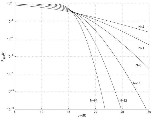
(a) $m=1$, $N=2,4,8,16,32,64$.

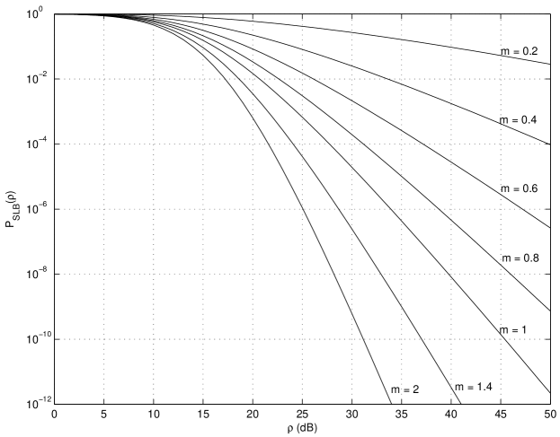
(b) $N=4$, $m=0.2,0.4,0.6,0.8,1,1.4,2$.

Figure 2: Sphere lower bound $P_{\rm slb}(\rho)$ for various values of $N$ and $m$.

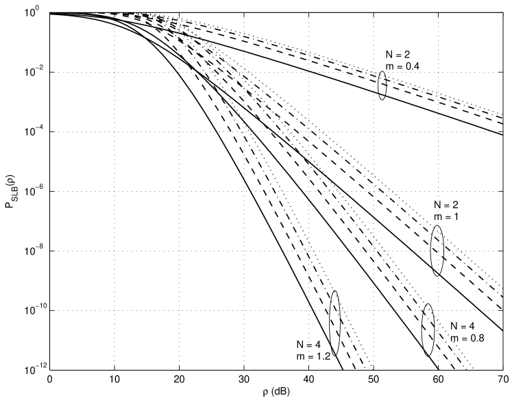
Figure 3: Sphere lower bound $P_{\rm slb}(\rho)$ for $L=1$ (solid), $L=10$ (dashed), $L=100$ (dashed-dotted) and $L=1000$ (dotted) and various values of $N$ and $m$.

For $N>1$ a closed form inverse transform of this function is not available, but we can nevertheless compute the pdf $p_{\zeta}(z)$ numerically by using an inverse fast Fourier transform (FFT). As an example, Figures 2 show the SLB for $L=1$ for various values of $N$ and $m$. As anticipated by Theorem 1, the curves get steeper as $m$ or $N$ increase. Moreover, Figure 3 shows the SLB for $L=1,10,100,1000$ and various values of $N$ and $m$. For a given $N$ and $m$, all curves have the same diversity. Observe that as $L$ increases the SLB increases, in contrast to what happens in the coded case, where as $L$ increases, the SLB converges to the outage probability of the channel, as demonstrated in [10]. We note that the SNR $\rho=1/\sigma^{2}$ is relative to the infinite lattice with vol$(\Lambda)=1$, since the average transmitted energy cannot be defined.

IV Performance of rotated lattices

In this section, we give a number of examples that use the SLB as a benchmark for comparing some lattices obtained by algebraic rotations, as explained in section II-A. In particular, we will use the best known or optimal algebraically rotated ${\mathbb{Z}}^{N}$ lattices in terms of largest minimum product distance [1, 2, 16, 3]. As we shall see, these rotations perform very close to the lower bound. Furthermore, we will show that the ensemble of random rotations does not have full diversity. This highlights the role of specific constructions that guarantee full diversity and largest minimum product distance for approaching the SLB.

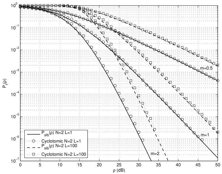
Figure 4: Frame error probability $P_{\rm f}(\rho)$ and sphere lower bound $P_{\rm slb}(\rho)$ for $N=2$, $m=0.5,1,2$ and $L=1,100$.

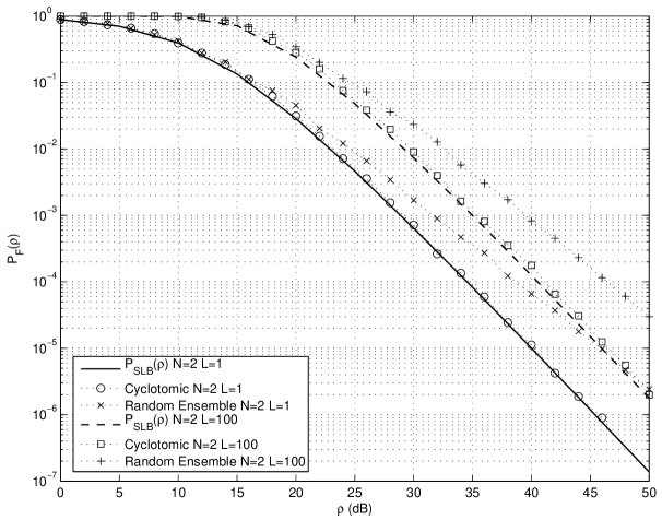
(a) Cyclotomic and average over Haar ensemble for $L=1,100$.

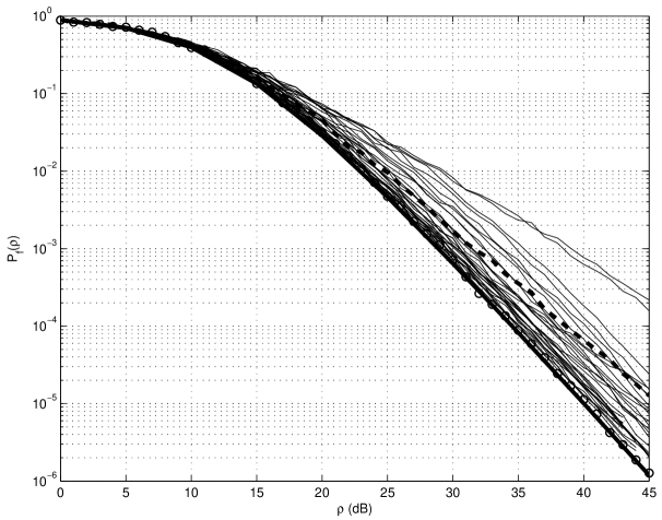
(b) 30 random samples from the Haar ensemble for $L=1$. The SLB (thick solid), average over random rotations (thick dashed) and Cyclotomic (circles) are shown for reference

Figure 5: Frame error probability $P_{\rm f}(\rho)$ and sphere lower bound $P_{\rm slb}(\rho)$ for $N=2$, $m=1$ and $L=1,100$.

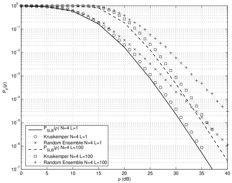
Figure 6: Frame error probability $P_{\rm f}(\rho)$ and sphere lower bound $P_{\rm slb}(\rho)$ for $m=1$, $N=4$, $L=1,100$ with Krüskemper rotation.

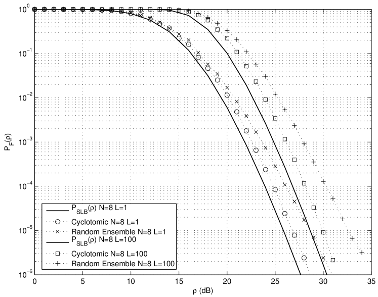
Figure 7: Frame error probability $P_{\rm f}(\rho)$ and sphere lower bound $P_{\rm slb}(\rho)$ for $m=1$, $N=8$, $L=1,100$ with cyclotomic rotation.

To illustrate this, Figures 4, 5, 6 and 7, compare the frame error probability $P_{\rm f}(\rho)$ of optimal rotations with largest minimum product distance (see [1, 2, 16] for more information on optimal constructions) obtained by simulation of the infinite lattice using a Schnorr-Euchner decoder [17] with the $P_{\rm slb}(\rho)$. The corresponding rotation matrices are also available in [3]. In particular, Figure 4 compares the performance of the cyclotomic rotation for $N=2$ and $L=1,100$ and $m=0.5,1,2$. Figures 6 and 7 show the SLB and the optimal rotations for $N=4,8$, namely the Krüskemper and cyclotomic rotations respectively [1, 2, 16]. As we observe, optimal rotations are very close to the SLB. As $N$ increases, algebraic rotations with largest minimum product distance show some gap to $P_{\rm slb}(\rho)$. This is due to the fact that for large $N$, the minimum product distance is not the only relevant design parameter for optimizing the coding gain. Without any loss of generality in the presentation of our results, from now on, and unless otherwise specified, forthcoming examples will be shown for $m=1$.

Figures 5(a), 6 and 7 also compare by simulation the performance of the aforementioned full-diversity algebraic rotations with the average performance of the ensemble of random rotations. To compute it, at every frame we generate a random matrix ${\bf A}$ with zero mean and unit variance i.i.d. Gaussian entries. We then perform a ${\bf A}={\bf Q}{\bf R}$ decomposition and let ${\bf M}={\bf Q}$. This is the simplest way of generating the ensemble of random rotations (orthogonal matrices) with the Haar distribution [18, 19]. As we observe, algebraic rotations perform very close to $P_{\rm slb}(\rho)$. On the other hand, the average error probability over the ensemble of random rotations, lacks of the full diversity and shows bad performance. To better understand this behavior, Figure 5(b) shows the simulated performance of 30 random samples of the Haar ensemble for $N=1$ and $L=1$, compared to the SLB (thick solid line), performance of the cyclotomic rotation (circles) and the ensemble average (thick dashed line). We observe that almost all instances have full diversity (though with very different coding gains). However, the ensemble average performance is dominated by bad rotation matrices. In particular, a closer look to the two worse curves reveals that the corresponding rotation matrices are very close to the identity, achieving effectively no rotation nor diversity. Furthermore, we observe that as $N$ increases, the performance of random rotations improves, despite showing a different asymptotic slope. This is due to the fact that for large $N$, there is a lot of diversity in the channel and the error probability curves get very steep. This means that for large $N$, random rotations will perform well for low-to-medium SNR.

V Performance of multidimensional signal sets

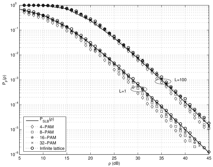
Figure 8: Frame error probability $P_{\rm f}(\rho)$ of the finite constellation generated with $4,8,16,32$-PAM, $P_{\rm f}(\rho)$ with $N=2$ of the infinite lattice and sphere lower bound $P_{\rm slb}(\rho)$ for $L=1,100$ with the cyclotomic rotation.

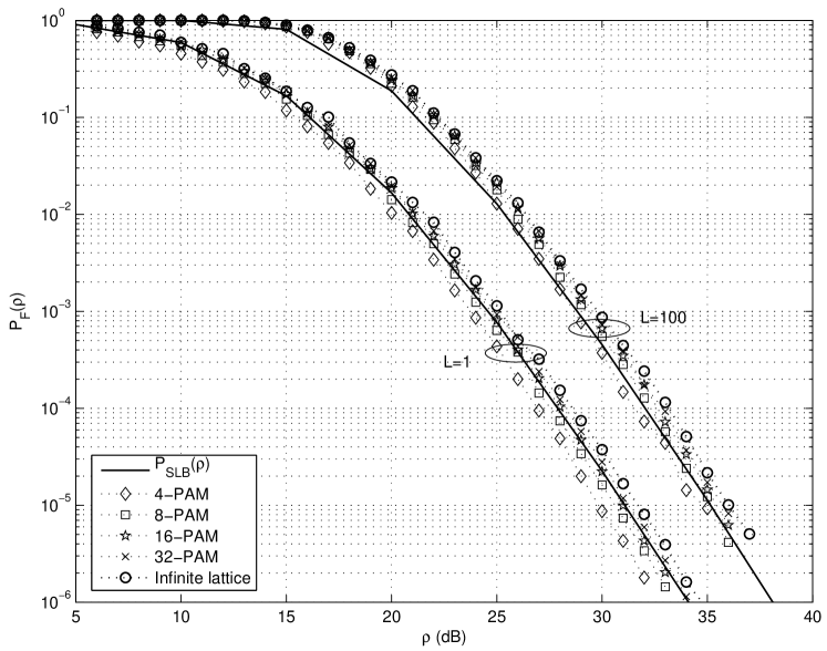
Figure 9: Frame error probability $P_{\rm f}(\rho)$ of the finite constellation generated with $4,8,16,32$-PAM, $P_{\rm f}(\rho)$ with $N=4$ of the infinite lattice and sphere lower bound $P_{\rm slb}(\rho)$ for $L=1,100$ with the Krüskemper rotation.

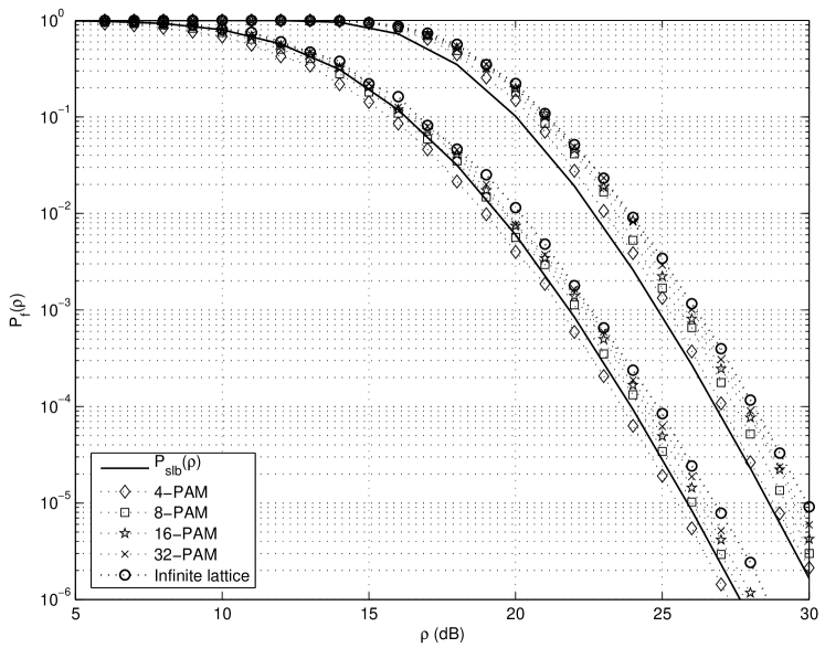
Figure 10: Frame error probability $P_{\rm f}(\rho)$ of the finite constellation generated with $4,8,16,32$-PAM, $P_{\rm f}(\rho)$ with $N=8$ of the infinite lattice and sphere lower bound $P_{\rm slb}(\rho)$ for $L=1,100$ with the cyclotomic rotation.

Practical systems use finite signal alphabets and the performance of the infinite rotated lattice should serve mainly as a guideline. Unfortunately, we do not have a bound similar to $P_{\rm slb}(\rho)$ for the finite case to take into account the boundary effects. We conjecture that the best multidimensional signal set using $M$-PAM is the one that has generator matrix ${\bf M}$ such that $P_{\rm f}(\rho)$ is closest to $P_{\rm slb}(\rho)$ for large enough $\rho$. As we shall see in the following example, as $M$ increases, the performance of the multidimensional signal constellation approaches that of the infinite rotated lattice, despite the boundary effects. This is precisely the continuity argument used in [8] for lattice codes. Indeed, Figures 8, 9 and 10 show the performance for $N=2,4,8$ and $L=1,100$ of the signal constellations obtained from $M$-PAM with the optimal algebraic rotation. In the comparison with the infinite lattice (circles) and $P_{\rm slb}(\rho)$, we observe all curves are within $1.5$ dB. Note that the SNR axis does not take into account the different average energies of the finite constellations and that we assume that the minimum distance of the $M$-PAM is $1$ for comparison to the infinite lattice lower bound. In order to plot the performance in terms of $\frac{E_{b}}{N_{0}}=\frac{E_{b}}{2}\rho$ it is enough to shift the curves by

$$10\log_{10}\left(\frac{M^{2}-1}{24\log_{2}M}\right)\rm dB$$

VI Conclusions

In this paper we have studied the performance of multidimensional rotated lattice constellations. We have applied the sphere lower bound for the infinite lattice to the block-fading channel and proved that the bound has full diversity. We have shown that optimally rotated algebraic lattices perform very close to the bound, while the average over the ensemble of random rotations does not. Furthermore, we have shown that finite constellations obtained from the rotation of $\{M\!-\!\mbox{PAM}\}^{N}$ constellations perform close to the bound as $M$ gets large. We have conjectured that optimal multidimensional signal sets with $M$-PAM constellation are obtained from rotated lattices whose performance is closest to the sphere lower bound.

Appendix A: Proof of Theorem 1

The exponential equality $\doteq$ and inequalities $\dot{\geq}$ and $\dot{\leq}$ were introduced in [20]. We write $f(z)\doteq z^{d}$ to indicate that $\lim_{z\rightarrow\infty}\frac{\log f(z)}{\log z}=d$. The exponential inequalities $\dot{\geq}$ and $\dot{\leq}$ are defined similarly. The function $\leavevmode\hbox{\small 1\normalsize\kern-3.30002pt1}\{{\cal E}\}$ is the indicator function of the event ${\cal E}$, namely, $\leavevmode\hbox{\small 1\normalsize\kern-3.30002pt1}\{{\cal E}\}=1$ when ${\cal E}$ is true, and zero otherwise. Following [20], we define the normalized fading gains $\alpha_{n}\stackrel{{\scriptstyle\Delta}}{{=}}-\frac{\log\gamma_{n}}{\log\rho}$. It is not difficult to show that the joint pdf of the vector ${\mbox{\boldmath$\alpha$}}=(\alpha_{1},\dotsc,\alpha_{N})$ is given by,

$$p({\mbox{\boldmath$\alpha$}})=\left(\frac{m^{m}\log\rho}{\Gamma(m)}\right)^{N}e^{-m\sum_{n=1}^{N}\rho^{-\alpha_{n}}}\rho^{-m\sum_{n=1}^{N}\alpha_{n}}.$$

Using the same arguments as in [20, 21, 22] we have that asymptotically for large $\rho$

$$p({\mbox{\boldmath$\alpha$}})\doteq\rho^{-m\sum_{n=1}^{N}\alpha_{n}}$$

for ${\mbox{\boldmath$\alpha$}}\in{\mathbb{R}}^{N}_{+}$, where ${\mathbb{R}}_{+}$ are the positive reals including zero. We can express the SLB as,

$$P_{\rm slb}(\rho)=1-\int_{{\mathbb{R}}^{N}}\left[1-\overline{\Gamma}\left(\frac{N}{2},\beta({\mbox{\boldmath$\alpha$}})\right)\right]^{L}p({\mbox{\boldmath$\alpha$}})d{\mbox{\boldmath$\alpha$}}$$ (9)

where

$$\beta({\mbox{\boldmath$\alpha$}})\stackrel{{\scriptstyle\Delta}}{{=}}\frac{1}{2\pi}\Gamma\left(\frac{N}{2}+1\right)^{\frac{2}{N}}\rho^{1-\frac{1}{N}\sum_{n=1}^{N}\alpha_{n}}$$ (10)

is the second argument of the incomplete Gamma function in (7) as a function of $\alpha$. Since $0\leq\left[1-\overline{\Gamma}\left(\frac{N}{2},\beta({\mbox{\boldmath$\alpha$}})\right)\right]^{L}\leq 1$ we can apply the dominated convergence theorem [23] and write

$$\displaystyle\lim_{\rho\to\infty}\int_{{\mathbb{R}}^{N}}\left[1-\overline{\Gamma}\left(\frac{N}{2},\beta({\mbox{\boldmath$\alpha$}})\right)\right]^{L}p({\mbox{\boldmath$\alpha$}})d{\mbox{\boldmath$\alpha$}}~{}=~{}\displaystyle\int_{{\mathbb{R}}^{N}}\lim_{\rho\to\infty}\left[1-\overline{\Gamma}\left(\frac{N}{2},\beta({\mbox{\boldmath$\alpha$}})\right)\right]^{L}p({\mbox{\boldmath$\alpha$}})d{\mbox{\boldmath$\alpha$}}.$$

Therefore, since

$$\lim_{\rho\to\infty}\beta({\mbox{\boldmath$\alpha$}})=\begin{cases}0&\text{if $\sum_{n=1}^{N}\alpha_{n}>N$}\\ \infty&\text{if $\sum_{n=1}^{N}\alpha_{n}<N$}\end{cases}$$ (11)

we have that

$$\lim_{\rho\to\infty}\overline{\Gamma}\left(\frac{N}{2},\beta({\mbox{\boldmath$\alpha$}})\right)=\begin{cases}1&\text{if $\sum_{n=1}^{N}\alpha_{n}>N$}\\ 0&\text{if $\sum_{n=1}^{N}\alpha_{n}<N,$}\end{cases}$$ (12)

which implies that

$$\lim_{\rho\to\infty}1-\left[1-\overline{\Gamma}\left(\frac{N}{2},\beta({\mbox{\boldmath$\alpha$}})\right)\right]^{L}=\begin{cases}1&\text{if $\sum_{n=1}^{N}\alpha_{n}>N$}\\ 0&\text{if $\sum_{n=1}^{N}\alpha_{n}<N$}\end{cases}$$ (13)

and means that for any $L\geq 1$, the contribution to $P_{\rm slb}(\rho)$ from $\alpha$ such that $\sum_{n=1}^{N}\alpha_{n}<N$ is negligible for large $\rho$. Also, since $p({\mbox{\boldmath$\alpha$}})\dot{=}\rho^{-m\sum_{n=1}^{N}\alpha_{n}}$, we can write that, for every $L\geq 1$,

$$P_{\rm slb}(\rho)=\int_{{\mbox{\boldmath$\alpha$}}\in{\mathbb{R}}^{N}}p({\mbox{\boldmath$\alpha$}})d{\mbox{\boldmath$\alpha$}}~{}\doteq~{}\int_{{\mbox{\boldmath$\alpha$}}\in{\cal A}\cap{\mathbb{R}}^{N}_{+}}\rho^{-m\sum_{n=1}^{N}\alpha_{n}}d{\mbox{\boldmath$\alpha$}}$$ (14)

where ${\cal A}=\left\{{\mbox{\boldmath$\alpha$}}\in{\mathbb{R}}^{N}:\sum_{n=1}^{N}\alpha_{n}>N\right\}$. Therefore the diversity order of the SLB is given by

$$d=-\lim_{\rho\to\infty}\frac{1}{\log\rho}\log\int_{{\mbox{\boldmath$\alpha$}}\in{\cal A}\cap{\mathbb{R}}^{N}_{+}}\exp\left(-m\log\rho\sum_{n=1}^{N}\alpha_{n}\right)d{\mbox{\boldmath$\alpha$}}$$ (15)

We now apply Varadhan’s lemma [24] and we obtain that

$$d =\inf_{\alpha\in{\cal A}\cap{\mathbb{R}}^{N}_{+}}\left\{m\sum_{n=1}^{N}\alpha_{n}\right\}=m\inf_{\alpha\in{\cal A}\cap{\mathbb{R}}^{N}_{+}}\left\{\sum_{n=1}^{N}\alpha_{n}\right\}=mN$$ (16)

which completes the proof.

Appendix B: Distribution of $\zeta$

Consider the random variable $\gamma$ with pdf

$$p_{\gamma}(x)=\frac{m^{m}x^{m-1}}{\Gamma(m)}e^{-mx}$$

for $x,m>0$, then the cdf of $\log\gamma$ can be expressed as

$$\Pr(\log\gamma\leq x) =P_{\gamma}(e^{x})$$ (17)

$$=1-\overline{\Gamma}(m,me^{x})$$ (18)

and the pdf of $\log\gamma$ is given by

$$p_{\log\gamma}(x)=\frac{m^{m}}{\Gamma(m)}e^{m(x-e^{x})}~{}~{}~{}~{}-\infty<x<\infty$$

The corresponding characteristic function can be written as

$$G(f) ={\mathbb{E}}[e^{-j2\pi fx}]$$

$$=\int_{-\infty}^{+\infty}e^{-j2\pi fx}\frac{m^{m}}{\Gamma(m)}e^{m(x-e^{x})}\,dx$$ (19)

where using the change of variables $y=me^{x}$ yields

$$G(f) =\int_{0}^{+\infty}\frac{m^{j2\pi f-1}}{\Gamma(m)}y^{m-1-j2\pi f}e^{-y}dy$$ (20)

$$=\frac{m^{j2\pi f-1}}{\Gamma(m)}\Gamma(m-j2\pi f).$$ (21)

Finally, the characteristic function of $\zeta$ is given by

$$G_{\zeta}(f)=\left(\frac{m^{j2\pi f-1}}{\Gamma(m)}\Gamma(m-j2\pi f)\right)^{N}.$$

Figure 11 shows $p_{\zeta}(z)$ evaluated numerically. In particular, Figure 11(a) shows the $p_{\zeta}(z)$ for different values of $N$ and $m=1$ while Figure 11(b) shows $p_{\zeta}(z)$ for $N=8$ and different values of $m$.

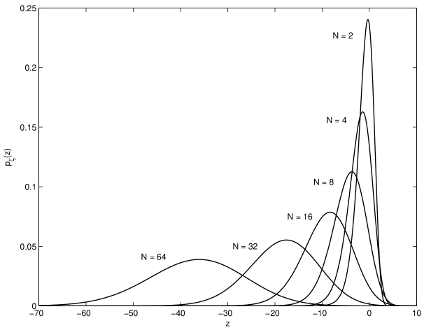
(a) $m=1$, $N=2,4,8,16,32,64$.

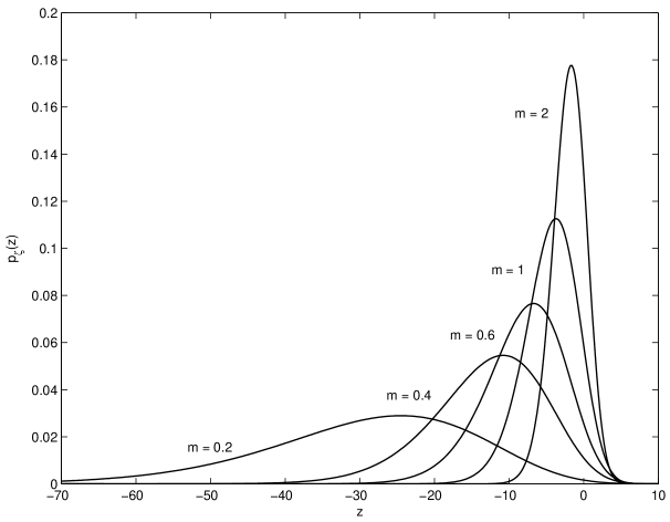
(b) $N=8$, $m=0.2,0.4,0.6,1,2$.

Figure 11: Probability density function $p_{\zeta}(z)$ for various values of $N$ and $m$.

References

- [1] E. Bayer-Fluckiger, F. Oggier, E. Viterbo, “New algebraic constructions of rotated -lattice constellations for the Rayleigh fading channel,” IEEE Trans. on Inf. Theory, vol. 50, no. 4, pp. 702–714, Apr. 2004.
- [2] F. Oggier and E. Viterbo, Algebraic Number Theory And Code Design For Rayleigh Fading Channels, Foundations and Trends in Communications and Information Theory. Now Publishers Inc, 2004.
- [3] E. Viterbo and F. Oggier, “Tables of algebraic rotations,” http://www.tlc.polito.it/viterbo.
- [4] J.-C. Belfiore and E. Viterbo, “Approximating the error probability for the independent Rayleigh fading channel,” in 2005 International Symposium on Information Theory, Adelaide, Australia, Sept. 2005.
- [5] J. H. Conway and N. J. A. Sloane, Sphere packings, lattices and groups, Springer, 3rd edition, 1999.
- [6] C. E. Shannon, “Probability of error for optimal codes in a gaussian channel,” The Bell System Technical Journal, vol. 38, no. 3, pp. 279–324, May 1959.
- [7] E. Viterbo and E. Biglieri, “Computing the voronoi cell of a lattice: The diamond-cutting algorithm,” IEEE Trans. on Inf. Theory, vol. 42, no. 1, pp. 161–171, Jan. 1996.
- [8] V. Tarokh, A. Vardy and K. Zeger, “Universal bound on the performance of lattice codes,” IEEE Trans. on Inf. Theory, vol. 45, no. 2, pp. 670–681, Mar. 1999.
- [9] S. Vialle and J. Boutros, “Performance of optimal codes on Gaussian and Rayleigh fading channels: a geometrical approach,” in 37th Allerton Conf. on Commun., Control and Comput., Monticello, IL., Sept. 1999.
- [10] M. Fozunbal, S. W. McLaughlin and R. W. Schafer, “On performance limits of space-time codes: a sphere-packing bound approach,” IEEE Trans. on Inf. Theory, vol. 49, no. 10, pp. 2681–2687, Oct. 2003.
- [11] I. E. Telatar, “Capacity of multi-antenna Gaussian channels,” European Trans. on Telecomm., vol. 10, no. 6, pp. 585–596, November 1999.
- [12] L. H. Ozarow, S. Shamai and A. D. Wyner, “Information theoretic considerations for cellular mobile radio,” IEEE Trans. on Vehicular Tech., vol. 43, no. 2, pp. 359–378, May 1994.
- [13] J. Proakis, Digital Communications, McGraw-Hill, 4th edition, 2001.
- [14] M. Abramowitz and I. A. Stegun, Handbook of Mathematical Functions with Formulas, Graphs and Mathematical Tables, New York: Dover Press, 1972.
- [15] M. K. Simon and M. S. Alouini, Digital Communication over Fading Channels, John Wiley: New York, 2000.
- [16] F. Oggier, Algebraic methods for channel coding, Ph.D. thesis, Ecole Polytechnique Fédérale de Lausanne (EPFL), 2005.
- [17] E. Agrell, T. Eriksson, A. Vardy and K. Zeger, “Closest point search in lattices,” IEEE Trans. on Inf. Theory, vol. 48, pp. 2201–2214, Aug. 2002.
- [18] G. W. Stewart, “The efficient generation of random orthogonal matrices with an application to condition estimation,” SIAM J. Numer. Anal., vol. 17, pp. 403–409, 1980.
- [19] A. M. Tulino and S. Verdú, Random Matrix Theory and Wireless Communications, Foundations and Trends in Communications and Information Theory. Now Publishers Inc, 2004.
- [20] L. Zheng and D. Tse, “Diversity and multiplexing: A fundamental tradeoff in multiple antenna channels,” IEEE Trans. on Inf. Theory, vol. 5, no. 49, pp. 1073–1096, May 2003.
- [21] A. Guillén i Fàbregas and G. Caire, “Coded modulation in the block-fading channel: Coding theorems and code construction,” IEEE Trans. on Inf. Theory, vol. 52, no. 1, pp. 91–114, Jan. 2006.
- [22] K. D. Nguyen, A. Guillén i Fàbregas and L. K. Rasmussen, “A Tight Lower Bound to the Outage Probability of Block-Fading Channels,” submitted to IEEE Trans. Inf. Theory, 2007.
- [23] R. Durrett, Probability: Theory and Examples, Duxbury Press, 1996.
- [24] A. Dembo and O. Zeitouni, Large Deviations Techniques and Applications, Number 38 in Applications of Mathematics. Springer Verlag, 2nd edition, April 1998.