Quintessential inflation from 5D warped product spaces on a dynamical foliation

Abstract

Assuming the existence of a 5D purely kinetic scalar field on the class of warped product spaces we investigate the possibility of mimic both an inflationary and a quintessential scenarios on 4D hypersurfaces, by implementing a dynamical foliation on the fifth coordinate instead of a constant one. We obtain that an induced chaotic inflationary scenario with a geometrically induced scalar potential and an induced quasi-vacuum equation of state on 4D dynamical hypersurfaces is possible. While on a constant foliation the universe can be considered as matter dominated today, in a family of 4D dynamical hypersurfaces the universe can be passing for a period of accelerated expansion with a deceleration parameter nearly -1. This effect of the dynamical foliation results negligible at the inflationary epoch allowing for a chaotic inflationary scenario and becomes considerable at the present epoch allowing a quintessential scenario.

I Introduction

Added interest in theories of gravity in more than four dimensions comes from the fact that matter in 4D has a geometrical origin on this scenarios. Among these theoretical settings one can find the induced-matter theory Wess1 ; Wess1A ; Wess1B and the braneworld scenarios Maa1 ; Maa1A . The basic idea in the induced-matter theory is that our 4D universe is embedded in a 5D space-time in apparent vacuum. The latest condition is understood by the Ricci-flat metric restriction $R_{AB}=0$. In physical terms it means that sources of matter in 4D can be geometrically explained by using just one extended extra dimension assuming a 5D apparent vacuum. Braneworld scenarios can be basically represented by two models. One is the Arkani-Hamed-Dimopoulos-Dvali Dim1 ; Dim1A and the other are the Randall-Sundrum braneworld models I and II RS12 ; RS12A . In the context of braneworld models our universe is embedded in a higher dimensional space-time called the bulk while our observable universe lies on a 4D brane hypersurface. The main motivation of the Randall-Sundrum model I is to solve the gauge hierarchy problem in a geometrical manner instead of using symmetry principles Maa1 ; Maa1A . Metrics in Randall-Sundrum models and in general in braneworld scenarios are constructed employing the class of warped product metrics. This fact makes important the study of this kind of metrics even in other theories of gravitation.

Matter confinement in braneworld cosmologies yields a cosmological evolution in the brane which is different from the typical FRW evolution generating problems for instance with the usual nucleosynthesis scenario Lan . In an attempt of finding a solution to this problem a negative cosmological constant in the bulk was introduced generating a fine tuning between the brane tension and the bulk cosmological constant. This fine-tuning is an undesirable characteristic of many braneworld models. This kind of problems suggested the study of cosmological braneworld models with dynamical fields in the bulk. Among them we can find models with bulk scalar fields.

As it was shown in Mio1 when we consider a 5D purely kinetic scalar field on warped product spaces, it is possible to recover a standard inflationary scenario on 4D hypersurfaces given by establishing a constant foliation on the fifth coordinate, where the scalar potential of the inflaton field is geometrically induced and the equation of state of the induced matter is given by $P_{IM}=-\rho_{IM}$. There quantum confinement of the inflaton modes is achieved naturally for at least a class of warping factors. However there is no possibility to apply that formalism to describe in the same model the inflationary phase and the present period of accelerated expansion of the universe known as quintessential expansion .

A great quantity of cosmological data accumulated during the last years are supporting the idea that nowadays the universe is passing for a phase of accelerated expansion. The Hubble diagram of Type Ia Supernovae (SNeIa), measured by both the Supernovae Cosmology Project and the High-z Team up to redshift $z\sim 1$, was the first evidence that the expansion of the universe is currently accelerated Salvatore . The simplest explanation of this phenomena is the cosmological constant $\Lambda$. However in the $\Lambda$CDM cosmological model it is not clear why the inferred value of $\Lambda$ is 120 orders of magnitude lower with respect to the value inferred in particle physics. As another tentative solution many authors have proposed to replace the cosmological constant with a scalar field rolling down its potential generating a model known as quintessence Pad .

In this letter we are interested in investigate the possibility to extend the formalism developed in Mio1 in order to study quintessential and inflationary scenarios in a more geometrical manner. To achieve this we shall assume that the 5D space-time can be dynamically foliated by a family of 4D dynamical hypersurfaces $\Sigma:\psi=f(x^{0})$, being $\psi$ the space-like fifth coordinate and $x^{0}$ a time-like coordinate. The possibility of having dynamical hypersurfaces has been investigated by J. Ponce de Leon in JPLeon ; JPLeonA . In this letter we shall follow the Ponce de Leon’s mechanism of implementing dynamical foliations not just for 5D Ricci-flat metrics but for 5D warped product metrics. We have organized this letter as follows. Section I is a brief introduction. Section II is devoted to a general formalism describing how to implement dynamical foliations and induce effective scalar potentials geometrically on the class of warped product metrics. In section III we approach a cosmological scenario from a particular warped geometry. In subsections A and B, inflationary and quintessential scenarios are respectively obtained. Finally, section IV is reserved to some final comments and conclusions. In our conventions capital Latin indices run from 0 to 4, small Latin indices from 1 to 3 and Greek indices from 0 to 3. Also we adopt the metric signature $(+,-,-,-,-)$.

II General formalism

We consider a 5D space-time with metric $g_{AB}$, endowed with a purely kinetic scalar field $\varphi$ minimally coupled to gravity. Thus, in the local coordinates $y^{A}=(x^{\alpha},\psi)$ the 5D-action reads

$$^{(5)}{\cal S}=\int d^{\,4}x\,d\psi\,\sqrt{{}^{(5)}g}\left[\frac{{}^{(5)}R}{2\kappa^{2}}-\frac{1}{2}g^{AB}\varphi_{,A}\varphi_{,B}\right],$$ (1)

where ${}^{(5)}g$ is the determinant of the metric $g_{AB}$, ${}^{(5)}R$ is the scalar curvature and $\kappa$ being the 5D gravitational coupling. The field equations derived from the action (1) are of the form

$$G_{AB}=\kappa^{2}T_{AB},$$ (2)

$${}^{(5)}\Box\varphi\equiv\frac{1}{\sqrt{{}^{(5)}g}}\frac{\partial}{\partial x^{A}}\left[\sqrt{{}^{(5)}g}g^{AB}\varphi_{,B}\right]=0.$$ (3)

being $T_{AB}^{(\varphi)}=\varphi_{,A}\varphi_{,B}-\frac{1}{2}g_{AB}\varphi^{,C}\varphi_{,C}$ the energy momentum tensor for the purely kinetic scalar field $\varphi$ and $G_{AB}=R_{AB}-(1/2)g_{AB}\,^{(5)}R$ the 5D Einstein tensor.

Now let us to consider the class of warped geometries which are given by the line element

$$dS^{2}=e^{2A(\psi)}h_{\alpha\beta}dx^{\alpha}dx^{\beta}-d\psi^{2},$$ (4)

where the real value function $A(\psi)$ is a warping factor and the 4D-part $h_{\alpha\beta}$ of the 5D metric $g_{AB}$ does not depend of the fifth coordinate, i.e. $h_{\alpha\beta}=h_{\alpha\beta}(x)$. Clearly, in (4) the fifth coordinate $\psi$ has spatial units and $A(\psi)$ is dimensionless.

On this metric background equation (3) becomes

$$^{(4)}\Box\varphi-e^{-2A(\psi)}\frac{\partial}{\partial\psi}\left[e^{4A(\psi)}\frac{\partial\varphi}{\partial\psi}\right]=0,$$ (5)

where ${}^{(4)}\Box\varphi=(1/\sqrt{-h})(\partial/\partial x^{\mu})(\sqrt{-h}h^{\mu\nu})\varphi_{,\nu}$. Assuming separability of the scalar field $\varphi(x,\psi)=\Gamma(\psi)\phi(x)$, the dynamics of the field on the fifth dimension is determined by Mio1

$$\overset{\star\star}{\Gamma}+4\overset{\star}{A}(\psi)\overset{\star}{\Gamma}-\alpha e^{-2A(\psi)}\Gamma=0,$$ (6)

with $\alpha$ a separation constant and the star $(\star)$ denoting derivative with respect to the fifth dimension. This is a second order differential equation, which depending of the warping factor chosen in principle can be solved. Therefore, in general the 5D dynamics of $\varphi$ depends strongly of the class of warping factors considered.

In order to obtain the 4D effective dynamics, we consider a special family of 4D-hypersurfaces in the same manner as they were introduced by J. Ponce de Leon in JPLeon ; JPLeonA , called dynamical foliations. This way, assuming that the 5D space-time can be foliated by a family of dynamical hypersurfaces $\Sigma:\psi=\psi(x^{0})$, being $x^{0}$ a time-like local coordinate, the induced metric on $\Sigma$ reads

$$ds_{\Sigma}^{2}=\left[e^{2A[\psi(x^{0})]}h_{00}(x)-\left(\frac{d\psi}{dx^{0}}\right)^{2}\right](dx^{0})^{2}+e^{2A[\psi(x^{0})]}h_{ij}(x)dx^{i}dx^{j}.$$ (7)

Thus, in order to recover an effective 4D line element $ds^{2}=\gamma_{\mu\nu}(x)dx^{\mu}dx^{\nu}$ on the hypersurface $\Sigma$, whose explicit form depends of the problem addressed, the continuity of $g_{AB}$ across $\Sigma$ requires JPLeon ; JPLeonA

$$e^{2A[\psi(x^{0})]}h_{00}(x)-\left(\frac{d\psi}{dx^{0}}\right)^{2} = \gamma_{00}(x),$$ (8)

$$e^{2A[\psi(x^{0})]}h_{ij}(x) = \gamma_{ij}(x).$$ (9)

Solutions of (8) determine the dynamical foliations $\psi=\psi(x^{0})$ allowed by the 5D geometry, while equation (9) describes the contribution of every dynamical foliation $\psi=\psi(x^{0})$ to the 3D spatial part of the effective metric, $\gamma_{ij}(x)$.

On a generic hypersurface $\Sigma:\psi=\psi(x^{0})$, the effective 4D action reads

$$^{(4)}{\cal S}_{eff}=\int d^{4}x\sqrt{-\,^{(\Sigma)}\!g}\left[\,\frac{{}^{(4)}\!R_{\Sigma}}{16\pi G}+{\cal L}_{IM}+\,^{(e)}\!{\cal L}_{IM}+\frac{1}{2}\,^{(\Sigma)}\!g^{\alpha\beta}\varphi_{eff\,,\alpha}\varphi_{eff\,,\beta}-V(\varphi_{eff})\right],$$ (10)

where ${}^{(\Sigma)}g_{\alpha\beta}$ is the tensor metric on $\Sigma$, ${\cal L}_{IM}$ is a typical induced matter lagrangian density, ${}^{(e)}{\cal L}_{IM}$ is a new contribution to ${\cal L}_{IM}$ due to the dynamical foliation considered $\psi=f(x^{0})$, $\varphi_{eff}[x^{0},x^{i},f(x^{0})]=\left.\varphi(x,\psi)\right|_{\psi=f(x^{0})}$ is the effective scalar field induced on $\Sigma$ and the effective 4D induced scalar potential is given by

$$V(\varphi_{eff})=\left.\frac{1}{2}\left(\frac{\partial\varphi}{\partial\psi}\right)^{2}\right|_{\psi=f(x^{0})}=\frac{1}{2}\,m^{2}(t)\,\varphi_{eff}^{2},$$ (11)

being $m^{2}(t)=[\overset{\star}{\Gamma}(\psi)/\Gamma(\psi)]^{2}|_{\psi=f(t)}$ a dynamical mass associated to $\varphi_{eff}$ which is geometrical in origin.

III A cosmological scenario

Since we are interested in cosmological solutions, we will assume that the metric $h_{\alpha\beta}$ is spatially 3D homogeneous and isotropic. Choosing for simplicity $h_{\alpha\beta}$ as a spatially flat FRW metric, the 5D line element (4) becomes

$$dS^{2}=e^{2A(\psi)}\left[dt^{2}-a^{2}(t)dr^{2}\right]-d\psi^{2},$$ (12)

where $a(t)$ is the scale factor and $dr^{2}=dX^{2}+dY^{2}+dZ^{2}$, being $[X,Y,Z]$ cartesian coordinates. On a generic dynamical hypersurface $\Sigma_{c}:\psi=f(t)$ the induced 4D metric ${}^{(\Sigma_{c})}g_{\alpha\beta}$ is given by the line element

$$ds_{\Sigma_{c}}^{2}=\left[e^{2A[f(t)]}-\dot{f}^{2}(t)\right]dt^{2}-e^{2A[f(t)]}a^{2}(t)dr^{2},$$ (13)

with the dot denoting partial derivative with respect to the cosmic time $t$. In order to obtain a spatially flat FRW on the 4D hypersurface $\Sigma_{c}$, where the line element is

$$ds_{\Sigma_{c}}^{2}=dt^{2}-b^{2}(t)dr^{2},$$ (14)

the continuity conditions across $\Sigma_{c}$ (8) and (9) read

$$e^{2A[f(t)]}-\dot{f}^{2}(t) = 1,$$ (15)

$$e^{2A[f(t)]}a^{2}(t) = b^{2}(t),$$ (16)

being $b(t)$ an affective scale factor. In this case, we can see from equation (16) that the typical scale factor $a(t)$ is dynamically rescaled as a consequence of taking a dynamical foliation.

From the action (10) the effective 4D Friedmann equations on $\Sigma_{c}$ are

$$3\left(\frac{\dot{b}}{b}\right)^{2} = 8\pi G\left[\rho_{IM}+\rho_{e}+\rho_{s}\right],$$ (17)

$$2\frac{\ddot{b}}{b}+\left(\frac{\dot{b}}{b}\right)^{2} = -8\pi G\left[P_{IM}+P_{e}+P_{s}\right],$$ (18)

where the induced matter density and pressure $\rho_{IM}$ and $P_{IM}$, the extra density and pressure terms coming due to the dynamical foliation $\rho_{e}$ and $P_{e}$, and the density and pressure of the effective scalar field $\rho_{s}$ and $P_{s}$, are given by

$$\rho_{IM} = -P_{IM}=\frac{3}{8\pi G}(A^{\prime\prime}+2A^{\prime 2})$$ (19)

$$\rho_{e} = \frac{3}{8\pi G}\left[2\frac{\dot{b}}{b}A^{\prime}\dot{f}+(A^{\prime}\dot{f})^{2}\right]$$ (20)

$$P_{e} = -\frac{1}{8\pi G}\left[6A^{\prime}\frac{\dot{b}}{b}\dot{f}+(2A^{\prime\prime}+3A^{\prime 2})\dot{f}^{2}+2A^{\prime}\ddot{f}\right]$$ (21)

$$\rho_{s} = \frac{1}{2}\,\left(\dot{\varphi}_{eff}+\varphi^{\prime}_{eff}\dot{f}\right)^{2}+\frac{e^{2A(f)}}{2b^{2}}\left(\nabla_{r}\varphi_{eff}\right)^{2}+V(\varphi_{eff}),$$ (22)

$$P_{s} = \frac{1}{2}\,\left(\dot{\varphi}_{eff}+\varphi^{\prime}_{eff}\dot{f}\right)^{2}+\frac{e^{2A(f)}}{2b^{2}}\left(\nabla_{r}\varphi_{eff}\right)^{2}-V(\varphi_{eff})$$ (23)

where the prime $(^{\prime})$ denotes $(\partial/\partial\psi)$ evaluated at $\psi=f(t)$. Besides, the field equation for the effective 4D scalar field reads

$$\ddot{\varphi}_{eff}+3\frac{\dot{b}}{b}\dot{\varphi}_{eff}-e^{2A(f)}b^{-2}\nabla_{r}^{2}\varphi_{eff}+\frac{dV(\varphi_{eff})}{d\varphi_{eff}}+\left[2\dot{\varphi}^{\prime}_{eff}+3\frac{\dot{b}}{b}\varphi^{\prime}_{eff}-3A^{\prime}\dot{\varphi}_{eff}\right]\dot{f}+\left(\varphi^{\prime\prime}_{eff}-3A^{\prime}\varphi^{\prime}_{eff}\right)\dot{f}^{2}+2\varphi^{\prime}_{eff}\ddot{f}=0.$$ (25)

Hence, the 4D effective cosmological dynamics is described by equations (17), (18) and (25). Clearly, when we consider a constant foliation $\psi=\psi_{0}$ instead of a dynamical one, equations (17) and (18) reduce to the ones obtained in Mio1 , while equation (25) reduces to a typical scalar field equation for an effective scalar field $\varphi_{eff}$.

III.1 4D effective inflation

In order to obtain inflationary solutions on the scenario previously described, we consider a homogeneous effective scalar field, $(1/2)(\nabla_{r}\varphi_{eff})^{2}\ll V(\varphi_{eff})$. In addition we assume a type of slow-roll conditions $(1/2)(\dot{\varphi}_{eff}+\varphi^{\prime}_{eff}\dot{f})^{2}\ll V(\varphi_{eff})$. Thus, defining the total energy density $\rho_{T}$ and pressure $P_{T}$ respectively as $\rho_{T}=\rho_{IM}+\rho_{e}+\rho_{s}$ and $P_{T}=P_{IM}+P_{e}+P_{s}$, the general equation of state can be written as $P_{T}=\omega(t)\rho_{T}$ where

$$\omega(t)\simeq-\left[1+\frac{2A^{\prime\prime}\dot{f}^{2}+2A^{\prime}\ddot{f}}{3A^{\prime\prime}+6A^{\prime 2}+6A^{\prime}(\dot{b}/b)\dot{f}+(A^{\prime}\dot{f})^{2}+M_{Pl}^{-2}V(\varphi_{eff})}\right]$$ (26)

being $M_{Pl}=(8\pi G)^{-1/2}$ the reduced Planckian mass. As the dynamical foliation $\psi=f(t)$, according to (15), depends directly of the warping factor $A(\psi)|_{\psi=f(t)}$, we can say that in principle for every warping factor we have a different type of induced matter which satisfy the equation of state (26).

Now, in order to obtain a particular cosmological scenario let us to consider the warping factor $A(\psi)=ln(\psi/\psi_{0})$, with $\psi_{0}$ an arbitrary dimensionalization constant with units of lenght. Thus, the 5D line element (12) becomes

$$ds^{2}=\left(\frac{\psi}{\psi_{0}}\right)^{2}[dt^{2}-a^{2}(t)dr^{2}]-d\psi^{2}.$$ (27)

Solving equation (15) for this $A(\psi)$ we obtain the solutions

$$f(t)=\pm\psi_{0},\qquad f(t)=\frac{\psi_{0}}{2}\left[1+e^{-2\Delta t/\psi_{0}}\right]e^{\Delta t/\psi_{0}},$$ (28)

where $\Delta t=t-t_{0}$, being $t_{0}$ the time when inflation begins. The first two solutions correspond to constant foliations and the last corresponds to a dynamical one. On the other hand, as it is well-known the inflationary period is pretty short ( $\sim 10^{-35}\,seg$ ) Guth1 , this way during this epoch $\Delta t<<1$, thus the dynamical foliation in (28) can be approximated as $f(t)\simeq\psi_{0}[1-\left(\Delta t/\psi_{0}\right)^{2}]\simeq\psi_{0}$, which means that practically during inflation this dynamical foliation behaves as a constant foliation. This way according to (26) we can recover a quasi-vacuum equation of state $P_{T}\simeq-\rho_{T}$ during inflation.

With this warping factor, the equation (6) has the general solution

$$\Gamma(\psi)=C_{1}\psi^{\sigma}+C_{2}\psi^{-\sigma},$$ (29)

being $C_{1}$ and $C_{2}$ integration constants and $\sigma=(1/2)[-3+\sqrt{9-4\alpha\psi_{0}^{2}}\,]$. Choosing $C_{2}=0$ and using (11) the 4D induced potential reads

$$V(\varphi_{eff})=\frac{1}{2}\,m_{0}^{2}\,\varphi_{eff}^{2},$$ (30)

where $m_{0}=\sigma\psi_{0}^{-1}$ is a constant geometrical mass associated to the effective inflaton field $\varphi_{eff}$. Thus, the dynamical equation (25) reduces to

$$\ddot{\varphi}_{eff}+3H(t)\dot{\varphi}_{eff}-\frac{1}{a^{2}}\nabla_{r}^{2}\varphi_{eff}+m_{0}^{2}\varphi_{eff}=0.$$ (31)

This equation describes the typical dynamics on a chaotic inflationary scenario. Chaotic inflation is a well-studied scenario and its dynamics can be found for example in Linde1 ; Linde1A ; Linde1B ; Linde1C ; Linde1D . In our case the inflaton mass $m_{0}$ can have a realistic value. For $\alpha\simeq-0.9\times 10^{-11}\,yrs^{-2}$ and $\psi_{0}=0.5\times 10^{10}\,yrs=0.584\times 10^{60}M_{Pl}^{-1}$ the inflaton mass has the value $m_{0}\simeq 3\times 10^{-6}\,M_{Pl}$, which is a realistic value according to Linde2 .

III.2 A quintessential scenario

One of the current problems in modern cosmology is to explain the present period of accelerated expansion of the universe supported by numerous observations darke ; darkeA ; darkeB ; darkeC ; darkeD ; darkeE ; darkeF . A quintessential scenario can be obtained from the present formalism, where the quintessential accelerated expansion depends of the warping factor and is due to the dynamics of the fifth dimension i.e. it is due to we are considering a dynamical foliation of the warped 5D space-time.
The deceleration parameter $q$ using (16) reads

$$q=-\frac{\ddot{b}b}{\dot{b}^{2}}=-\frac{a\ddot{a}+a\left(\dot{a}A^{\prime}+A^{\prime\prime}\dot{f}+A^{\prime 2}\dot{f}\right)\dot{f}+aA^{\prime}\ddot{f}}{\left(\dot{a}+A^{\prime}\dot{f}\right)^{2}}.$$ (32)

At the present epoch $\Delta t\gg 1$, therefore the dynamical foliation (28) can be approximated by $f(t)\simeq(\psi_{0}/2)e^{\Delta t/\psi_{0}}$. Thus, considering $A(\psi)=ln(\psi/\psi_{0})$ and a power-law for $a(t)\simeq t^{p}$, the deceleration parameter (32) becomes

$$q=-\left[1-\frac{p\psi_{0}^{2}}{t^{2}+2p\psi_{0}t+p^{2}\psi_{0}^{2}}\right].$$ (33)

According to (32) and (33), the new contribution comes from the dynamical foliation $\psi=f(t)$. Thus we can say that a universe which is currently matter dominated $(p=2/3)$ on a constant foliation, can be now in a quintessential period on a dynamical one. Hence, for $H_{0}=0.7\times 10^{-10}yr^{-1}$, $t_{0}=1.4\times 10^{10}\,yrs$ and $\psi_{0}=0.5\times 10^{10}$, the deceleration parameter (33) at the present epoch would be $q_{0}=-0.9445$. The behavior of $q$ as a function of $t$ in the present epoch is shown in the figure [1]. We can see that $q$ tends asymptotically to $-1$ with time.
Inserting (32) in $\omega(t)=[2q(t)-1]/3$ we obtain

$$\omega(t)=-1+\frac{2p\psi_{0}^{2}}{3[t_{0}^{2}+2p\psi_{0}t_{0}+p^{2}\psi_{0}^{2}]},$$ (34)

which according to the previous data has the present value $\omega_{0}=-0.963$. These results fit into the current observational data according to data ; dataA ; dataB ; dataC

IV Final comments

In this letter we have investigated the possibility of mimic both the inflationary and the present quintessence epochs from a 5D warped product space equipped with a purely kinetic scalar field, by implementing a dynamical foliation instead of a constant one. We have obtained that if we consider a matter-dominated universe at the present time on the constant foliation $\Sigma_{0}:\psi=\psi_{0}$, it is possible to obtain a quintessential scenario where the accelerated expansion is geometrically generated by the dynamical foliation $\Sigma:\psi=f(t)$. The explicit form of the function $f(t)$ is given by the continuity conditions introduced by J. Ponce de Leon in JPLeon ; JPLeonA . For a warping factor of the form $A(\psi)=ln(\psi/\psi_{0})$ the dynamical foliation behaves as a constant one for early times and in particular during the inflationary phase. However it becomes completely dynamical at the present epoch generating geometrically a quintessential expansion with $q\simeq-1$. The 4D induced inflationary stage results a scenario of chaotic inflation with a geometrically induced scalar potential $V(\varphi_{eff})=(1/2)m_{0}^{2}\varphi_{eff}^{2}$, where a realistic value of $m_{0}\simeq 3\times 10^{-6}\,M_{Pl}$ can be achieved. Finally we show a plot with the behavior of the deceleration parameter $q$ during the quintessential period.

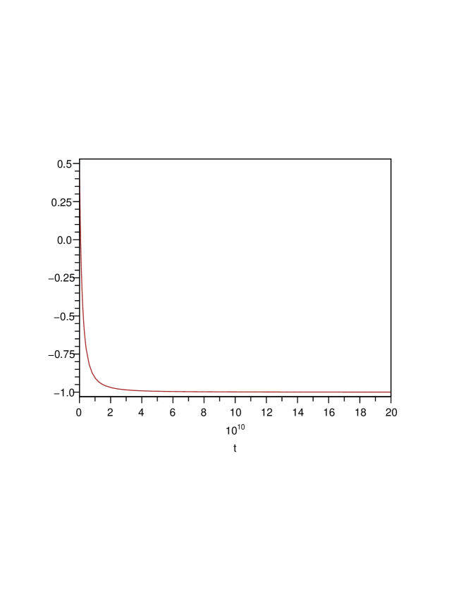
Figure 1: The figure shows the behavior of the deceleration parameter $q(t)$ with time $t$ during the present epoch, where we have taken $\psi_{0}=0.5\times 10^{10}\,yrs$, $p=2/3$ and t is given in years.

- (1) P. S. Wesson and J. Ponce de Leon, J. Math. Phys. (1992) 33 3883.
- (2) J. M. Overduin and P. S. Wesson, Phys. Rept. (1997) 283 303 [ArXiv: gr-qc/9805018].
- (3) P. S. Wesson, Space-Time-Matter (World Scientific, Singapore 1999).
- (4) R. Maartens, Living Reviews Relativity 7 (2004) [ArXiv: gr-qc/0312059].
- (5) Yoon-bai Kim, Chong Oh Lee, ll-bong Lee and Jung-Jai Lee, J. Kor. Astron. Soc. 37 (2004) 1-14.
- (6) N. Arkani-Hamed, S. Dimopoulos and G. Dvali, Phys. Lett. B429 (1998) 263.
- (7) I. Antoniadis, N. Arkani-Hammed, S. Dimopoulos and G. Dvali, Phys. Lett. B436 (1998) 257.
- (8) L. Randall and R. Sundrum, Phys. Rev. Lett. 83 (1999) 3370.
- (9) L. Randall and R. Sundrum, Phys. Rev. Lett. 83 (1999) 4690.
- (10) D. Langlois and Maria Rodriguez M., Phys. Rev. D64 (2001) 123507.
- (11) J. E. Madriz Aguilar, under review in Eur. Phys. J. C. [ArXiv: gr-qc/0704.2434].
- (12) S. Capozziello, Int. J. Geom. Meth. Mod. Phys. 4 (2007) 53-78, [ArXiv: astro-ph/0706.3587].
- (13) T. Padmanabhan, Phys. Rept. 380 (2003) 235.
- (14) J. Ponce de Leon, Mod. Phys. Lett. A21: 947-959, (2006), [ArXiv: gr-qc/0511067].
- (15) J. Ponce de Leon, Int. J. Mod. Phys. D15 (2006) 1237-1257.
- (16) A. H. Guth and D. I. Kaiser, Science 307, (2005) 884-890, [ArXiv: astro-ph/0502328].
- (17) Shinji Tsujikama, Lectures given at 2nd Tah Poe School on Cosmology: Modern Cosmology, Phitsanulok, Thailand, 17-25 Apr. (2003), ArXiv [hep-ph/0304257].
- (18) A. D. Linde, Phys. Lett. B129 (1983) 129-177.
- (19) A. D. Linde, JETP Lett. 38 (1983) 176-179.
- (20) A. D. Linde, Mod. Phys. Lett. A1 (1986) 81.
- (21) A. D. Linde, KOLB, E. W. (ED.), TURNER, M. S. (ED.): THE EARLY UNIVERSE (1988) 541-545.
- (22) A. Linde, Prog. Theor. Phys. Suppl. 163 (2006) 295-322.
- (23) T. Padmanabhan, AIP Conf. Proc. 861 (2006) 179-196.
- (24) S. Perlmutter et al., Astrophys. J. 517 (1999) 565.
- (25) R. A. Knop et al., Astrophys. J. 598 (2003) 102.
- (26) B. J. Barries et al., Astrophys. J. 602 (2004) 571.
- (27) A. G. Riess et al., Astrophys. J. 116 (1998) 1009.
- (28) J. L. Tonry et al., Astrophys. J. 594 (2003) 1.
- (29) S. Capozziello, Int. J. Geom. Meth. Mod. Phys. 4 (2007) 53-78.
- (30) D. N. Spergel et al., submitted to Astrophys. J. (2006) [ArXiv: astro-ph/0603449].
- (31) Review of Particle Physics, Phys. Rev. D66, (2002) 010001-170.
- (32) D. N. Spergel et al., Astrophys. J. Suppl. 148 (2003) 175.
- (33) Jeremiah P. Ostriker and T. Souradeep, Pramana 63 (2004) 817-828, [ArXiv: astro-ph/0409131].