First-order framework and domain-wall/brane-cosmology correspondence

Abstract

We address the possibility of finding domain wall solutions from cosmological solutions in brane cosmology. We find first-order equations for corresponding cosmology/domain wall solutions induced on 3-branes. The quadratic term of energy density in the induced Friedmann equation plays a non-standard role and we discuss the way the standard cosmological and domain wall models are recovered as the brane tension becomes large and show how they can be described by four-dimensional supergravity action in such a limit. Finally, we show that gravity on the 3-brane is locally localized as one moves away from the two-dimensional domain walls living on the brane.

I Introduction

The evolution of a 3-brane universe in the Randall-Sundrun scenario has been recently considered in the literature rs ; lcd ; defayet . The Einstein equations for braneworld cosmology admits a first integral that governs the cosmological evolution on the 3-brane, without any mention to the bulk evolution behavior. This first integral involves a modified Friedmann equation, in which the energy density contributes with both linear and quadratic terms. The trace of the five-dimensional spacetime is revealed at high energy by the quadratic term, whereas the four-dimensional standard cosmology is recovered in the low energy limit.

In this paper we consider the cosmological evolution on the 3-brane driven by a real scalar field. We are able to find first-order equations satisfying the equations of motion, by making a suitable choice of the scalar field potential written in terms of a ‘superpotential’ in a non-standard way, with the standard scalar potential of a four-dimensional supergravity theory being recovered at relatively low energy.

In order to make a correspondence between brane cosmology solutions and domain wall solutions living on the 3-brane, we consider the domain wall counterpart of the brane cosmology set up aforementioned, by carrying out analytic continuations which leads the time coordinate into a space coordinate on the 3-brane. At late times, the familiar scalar potential of a four-dimensional supergravity is recovered and then supergravity domain walls correspond to standard cosmology. In this regime the correspondence here falls into the framework already developed in Refs. mcvetic95 ; cvetic97 ; bglm ; abl ; st2006.1 ; st2006.2 .

Concerning the global behavior of the analytic continued 3-brane solution, our results show that gravity is localized on the 3-brane with the most concentration where there exists two-dimensional domain walls living in. As one goes far from such domain walls the gravity tends to be locally localized on the brane, i.e., after its falloff around the brane, the brane warp factor develops returning points and goes back to infinity just as in the Karch-Randall scenario kr . On the domain walls, the brane is flat assuming a four-dimensional Minkowski geometry rs , whereas far from the domain walls the brane is bent abl ; st2006.1 and assumes a four-dimensional Anti-de-Sitter ($AdS_{4}$) geometry – see, e.g., Refs. kalo ; st ; fwolf ; nunez ; alesio ; bbg2004 ; bbl2006 ; celi ; dalla ; cpv ; ber ; vau .

The paper is organized as follows. In Sec. II we present the first-order framework for non-standard brane cosmology and consider explicit examples. In Sec. III, we extend this framework for domain walls solutions by carrying out an analytic continuation and there we also consider some explicit examples. In Sec. IV, we show how the localization of gravity is affected by the localization of the two-dimensional domain walls on the brane. Finally in Sec. V we present our conclusions.

II First-order framework

In this paper we extend the first-order formalism recently considered in bglm to the case of the non-standard Friedmann equation which appears in brane cosmology lidsay ; ellis . The metric describing the cosmological evolution on a 3-brane is

$$ds_{5}^{2}=-n^{2}(t,r)dt^{2}+a^{2}(t,r)\gamma_{ij}dx^{i}dx^{j}+b^{2}(t,r)dr^{2},$$ (1)

where $\gamma^{ij}$ is a maximally symmetric 3-dimensional metric with spatial curvature $k=-1,0,1$. The five-dimensional Einstein equations are found for the action of a 3-brane embedded in a five-dimensional bulk, i.e.,

$$S_{5}\!=\!-\frac{1}{2\kappa_{5}^{2}}\!\!\int{\!d^{5}x\sqrt{-g}(R+\Lambda_{bulk})+\int{\!d^{5}x\sqrt{-g}\,\delta(r)}{\cal L}},$$ (2)

where ${\cal L}$ describe the dynamics on the brane. Below we shall assume $\kappa_{4}^{2}=8\pi G\simeq{\kappa_{5}^{4}\sigma}/{6}=2$. We are interested in the case where the five-dimensional bulk is an $AdS_{5}$ spacetime defayet , with the cosmological constant defined as $\rho_{bulk}\equiv\Lambda_{bulk}=-\sigma^{2}\kappa_{5}^{2}/6$ which satisfies the Randall-Sundrum fine tuning rs .

Let us start with the induced Friedmann equation on the brane given by

$$H^{2}=\frac{2}{3}\rho\left(1+\frac{\rho}{2\sigma}\right),$$ (3)

where $H={\dot{a}_{0}}/{a_{0}}$ and $a_{0}\!=\!a(t,r\!=\!0)$ is the scale factor on the brane worldvolume with the metric

$$ds_{4}^{2}=-dt^{2}+a_{0}^{2}(t)(dx^{2}+dy^{2}+dz^{2}).$$ (4)

Here $\rho$ is the energy density on the brane, $\sigma$ is the brane tension and $\rho_{bulk}\neq 0$ was recast in terms of $\sigma$. The quadratic nature of the density $\rho$ is due to junction condition across the 3-brane defayet embedded in the bulk with five dimensions. The equation involving the pressure $p$ is

$$\dot{H}=-(\rho+p)\left(1+\frac{\rho}{\sigma}\right).$$ (5)

The equations (3) and (5) can be found from the Einstein equations on the 3-brane maeda , ${}^{(4)}G_{\mu\nu}=-\Lambda_{4}q_{\mu\nu}+\kappa^{2}_{(4)}T_{\mu\nu}+\kappa^{4}_{(5)}\pi_{\mu\nu}-E_{\mu\nu}$, where $\Lambda_{4}$ and $q_{\mu\nu}$ are the cosmological constant and the metric on the brane, respectively. $\pi_{\mu\nu}$ is quadratic in the energy-momentum tensor $T_{\mu\nu}$ and $E_{\mu\nu}$ is part of the five-dimensional Weyl tensor. The standard cosmology is recovered as $\sigma$ becomes sufficiently large, i.e., $\kappa_{(5)}^{4}\sim 1/\sigma\sim 0$. Since, in our case, we are disregarding $\Lambda_{4}$ and $E_{\mu\nu}$, the brane dynamics in this regime is governed by the effective action

$$S^{\rm eff}_{4}=-\frac{1}{2\kappa^{2}_{(4)}}\int{d^{4}x\sqrt{-q}\,\left(\,{}^{(4)}R-2\kappa^{2}_{(4)}\cal{L}\,\right)}.$$ (6)

This equation will be useful for identifying a four-dimensional ‘supergravity’ action later. Let us now assume that the brane cosmology is driven by a scalar field whose Lagrangian density is

$${\cal L}=-\frac{1}{2}\partial_{\mu}\phi\partial^{\mu}\phi-V(\phi),$$ (7)

with $\mu=0,1,2,3.$ Thus, the familiar equations for the energy density $\rho$ and the pressure $p$ are

$$\rho=\frac{1}{2}\dot{\phi}^{2}+V(\phi),$$ (8)

$$p=\frac{1}{2}\dot{\phi}^{2}-V(\phi).$$ (9)

By applying the induced equation of conservation for the energy density on the brane, i.e., $\dot{\rho}+3H(\rho+p)=0$, we find

$$\dot{\rho}=-3H\dot{\phi}^{2}.$$ (10)

The scalar field dynamics is governed by the equation of motion

$$\ddot{\phi}+3H\dot{\phi}+\frac{\partial V}{\partial\phi}=0.$$ (11)

Since $\rho\equiv\rho(\phi)$, we use the fact that $\dot{\rho}=\rho^{\prime}(\phi)\dot{\phi}$, such that Eq. (10) becomes

$$\dot{\phi}=-\frac{\rho^{\prime}(\phi)}{3H}.$$ (12)

To get to the first-order equations, we follow the procedure of bglm , e.g. we introduce $W=W(\phi)$ and define $H={\dot{a}_{0}}/{a_{0}}=W(\phi)$, such that we have the following first-order equation

$$\frac{\dot{a}_{0}}{a_{0}}=W(\phi),$$ (13)

which allows us to rewrite the Eq. (3) in the form

$$\rho^{2}+2\sigma\rho-3\sigma W^{2}=0.$$ (14)

This algebraic equation has the following solutions

$$\rho_{\pm}={-\sigma\pm\sigma\sqrt{1+\frac{3W^{2}}{\sigma}}}.$$ (15)

We consider the solution with the upper sign, because of the positive energy condition. Thus, by differentiating the Eq. (15) it is not difficult to find that

$$\rho^{\prime}(\phi)=\frac{3WW_{\phi}}{\sqrt{1+\frac{3W^{2}}{\sigma}}}.$$ (16)

The above Eq. (12) can be now written as a first-order equation for the scalar field $\phi$ and the ‘superpotential’ $W$, i.e.,

$$\dot{\phi}=-\frac{W_{\phi}}{\sqrt{1+\frac{3W^{2}}{\sigma}}}.$$ (17)

One can easily check that the two first-order equations (13) and (17) satisfy the two second-order equations (5) and (11).

The scalar potential $V(\phi)$ can be found via Eqs. (8), (15) (upper sign), and (17). It has the explicit form

$$V(\phi)=-\sigma+\sigma\sqrt{1+\frac{3W^{2}}{\sigma}}-\frac{1}{2}\frac{W_{\phi}^{2}}{{1+\frac{3W^{2}}{\sigma}}}.$$ (18)

For a large brane tension $\sigma$, such that $W^{2}/\sigma\ll 1$, one can expand the potential in a power series as

$$V(\phi) = \frac{3}{2}W^{2}-\frac{1}{2}W_{\phi}^{2}+\frac{3}{2}W_{\phi}^{2}\frac{W^{2}}{\sigma}+\cdots$$ (19)

where the standard potential bglm is recovered by taking into account only the familiar quadratic terms

$$V(\phi) \simeq \frac{3}{2}W^{2}-\frac{1}{2}W_{\phi}^{2}.$$ (20)

Under similar approximations the standard first-order equation is recovered by turning on only linear terms in Eq. (17).

On the other hand, for small brane tension, such that $W^{2}/\sigma\gg 1$, the scalar potential approaches

$$V(\phi) \simeq \sigma\sqrt{\frac{3}{\sigma}}|W|,$$ (21)

and the first-order equation now reads

$$\dot{\phi}\simeq-\sqrt{\frac{\sigma}{3}}\frac{W_{\phi}}{|W|}.$$ (22)

Substituting (21) and (22) into the second-order equation (11), one finds that $\ddot{\phi}\simeq 0$, for $W>0$. This is precisely the slow-roll regime. Since $\ddot{\phi}\simeq 0$, thus for consistency $\dot{\phi}\simeq const.$ This implies that we can determine the ‘superpotential’, the inflaton solution for (22), and the scale factor solution for (13) given by

$$W(\phi)=V_{0}\,e^{\alpha\phi},\qquad\phi(t)=-\sqrt{\frac{\sigma}{3}}\,\alpha(t-t_{0}),\qquad a_{0}(t)=a_{0}\exp{\left[\frac{-V_{0}\sqrt{3}}{\alpha^{2}\sqrt{\sigma}}\exp{\left(\frac{-\alpha^{2}\sqrt{\sigma}}{\sqrt{3}}(t-t_{0})\right)}\right]},$$ (23)

where $\alpha$ and $V_{0}$ are constants, being $V_{0}^{2}/\sigma\gg 1$ consistent with the regime $W^{2}/\sigma\gg 1$. For $\alpha>0\,\,(\alpha<0)$, the Universe develops inflation at later (earlier) times $t<t_{0}$. The exponential potential is also consistent with string/M-theory.

Conversely, for $V_{0}^{2}/\sigma\ll 1$ one gets to the regime $W^{2}/\sigma\ll 1$, and the potential (21) and the first-order equation (22) do not make sense anymore. Instead, in this regime one recovers the previous analysis with the scalar potential (20). Thus $V_{0}^{2}/\sigma$ is assumed to be the coupling connecting asymptotic regimes of the exact potential (18) given in the form

$$V(\phi)=-\sigma+\sigma\sqrt{1+\frac{3V_{0}^{2}}{\sigma}\,e^{2\alpha\phi}}-\frac{1}{2}\frac{V_{0}^{2}\alpha^{2}e^{2\alpha\phi}}{{1+\frac{3V_{0}^{2}}{\sigma}\,e^{2\alpha\phi}}}.$$ (24)

As $\alpha>\sqrt{3}$, this potential develops a minimum at

$$\phi_{0}=\frac{1}{\alpha}\ln{\left[\frac{\sqrt{\alpha^{4/3}3^{1/3}\sigma-3\sigma}}{3V_{0}}\right]}.$$ (25)

To ease comparison, in Fig. 1 we depict the two regimes. Note that as $V_{0}^{2}/\sigma$ increases, the scalar potential approaches the form given in (21. On the other hand, as $V_{0}^{2}/\sigma$ decreases, the scalar potential (24) approaches the form (20). In this regime, the rolling inflaton field could eventually achieve the vacuum

$$\Lambda\equiv V(\phi_{0})=-\frac{1}{2}e^{2\alpha\phi_{0}}(-3+\alpha^{2})V_{0}^{2}.$$ (26)

It is clear from the equation above, that for $\alpha>\sqrt{3}$, one finds $\Lambda<0$, which corresponds to an $AdS_{4}$ vacuum. Moreover the negative vacuum at $\phi_{0}$ signalizes the possibility of the Universe undergoing an oscillatory expansion ts — see Fig. 1. Recall that, in our model, the Universe is infinite and flat $(k=0)$. For $\alpha<\sqrt{3}$, the potential has only the minimum $\phi_{0}=0$, and $\Lambda=-(1/2)(-3+\alpha^{2})V_{0}^{2}>0$ corresponds to a $dS_{4}$ vacuum. This produces inflation only at late times.

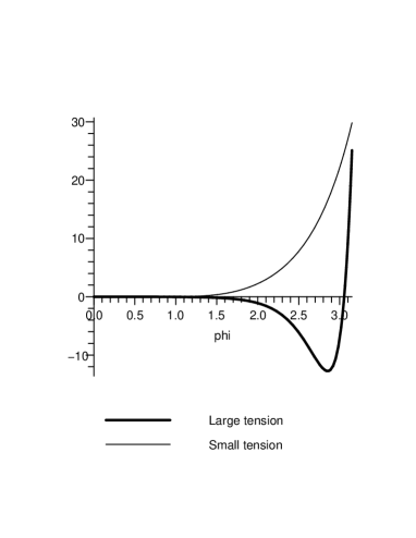
Figure 1: The scalar potential $V(\phi)$ for small ($\sigma=1$) and large ($\sigma=3\times 10^{3}$) tension, with $V_{0}=1/20$ and $\alpha=\sqrt{7/2}$. For large $\sigma$, the minimum occurs at $\phi_{0}=2.85$ such that our Universe (infinite and flat) can undergo an oscillatory expansion.

The cosmological scenario discussed above is particularly interesting, because the coupling $V_{0}^{2}/\sigma$ can vary as the brane inflates, such that the potentials pictured in Fig. 1 are asymptotic limits of a same scalar potential governing the brane evolution at high and low energy scales. However, other interesting cosmological scenarios are those where one fixes $V_{0}^{2}/\sigma=1$, which allows for a wider class of ‘superpotentials’. In the following we shall investigate such scenarios by using examples where $W\propto\sqrt{\sigma}$ all times.

II.1 Cosmological Examples

Given that many examples bglm ; abl ; st2006.1 ; st2006.2 have been previously considered in the literature for low energy limit of theory we describe above, let us now consider some examples for the exact theory. For $W(\phi)=\sqrt{\sigma/3}\sinh{\phi}$, the Eq. (17) is easily integrated whose solution is simply

$$\phi=-\sqrt{\frac{\sigma}{3}}(t-t_{0}).$$ (27)

The scale factor $a_{0}(t)$ on the brane can also be readily found by using the equation (13) and the solution (27). Its form is given by

$$a_{0}=\exp{\left[-\cosh{\sqrt{\frac{\sigma}{3}}}(t-t_{0})\right]}.$$ (28)

The larger is the brane tension (i.e., the standard cosmology regime), the later the inflation occurs. On the other hand, for small brane tension one deviates from the standard cosmology and inflation occurs only at earlier times — See Fig. 2. Note that the end of inflation occurs at a time $t_{0}$, with decelerating universe for $t>t_{0}$, in a way similar to the case of quadratic chaotic inflation models linde .

Figure 2: The scale factor $a_{0}(t)$ for $\sigma=1/2$ (thin line) and for $\sigma=1/5$ (thick line). The larger (smaller) $\sigma$ favors later (earlier) inflation. Note the end of inflation at $t_{0}=10$.

Let us now consider the example with $W(\phi)=\sqrt{\sigma/3}\tan{(\phi)}$. Here the solutions are given by

$$\phi=\mp\arcsin{\Big{(}\sqrt{\frac{\sigma}{3}}\mbox{$(t-t_{0})$}\Big{)}}$$ (29)

and

$${a_{0}}_{\pm}=\exp{\left[\pm\sqrt{-\frac{\sigma}{3}(t-t_{0})^{2}+1}\,\,\right]}.$$ (30)

The inflaton field (29) behaves in a singular way. The scale factor is depicted in Fig. 3. Note the two possibility of ‘limited’ expansion $a_{+}$ and $a_{-}$, with inflation beginning ($a_{0-}$) or ending ($a_{0+}$) at $t_{0}=10$.

Figure 3: The scale factor $a_{0\pm}(t)$ for $\sigma=1/20$ (thin line) and for $\sigma=1/30$ (thick line). Note the two possibility of limited expansion, with inflation beginning or ending at $t_{0}=10$.

III Domain-Wall/Brane-Cosmology Correspondence

It is now well-known that one can use cosmological solutions to find domain wall solutions, and vice-versa, by making use of analytic continuation cvetic93 ; cvetic97 ; ssakura2002 ; ssakura2002.1 ; st2006.1 ; st2006.2 .

All the developments above can be extended to give rise to domain wall solutions living on the four-dimensional brane world-volume. To carry out analytic continuation we make

$$W\to i\widetilde{W},$$ (31)

$$H\to i\widetilde{H},$$ (32)

$$t\to iy,$$ (33)

$$y\to it,$$ (34)

where $\widetilde{H}={a_{0}^{\prime}}/{a_{0}}=-\widetilde{W}.$ The original four-dimensional metric (4) describing cosmological solutions on the brane can now be written as

$$\!ds_{4}^{2}=dy^{2}+{a_{0}}^{2}(y)(-dt^{2}+dx^{2}+dz^{2}).$$ (35)

This metric represents solutions of two-dimensional flat domain walls within asymptotically four-dimensional Minkowski ($\mathbb{M}_{4}$) or anti-de Sitter (${AdS}_{4}$) spacetime cvetic93 ; cvetic97 . These domain walls are of current interest to cosmology spe ; co .

Since the domain wall solutions are analytic continued from the previous cosmological solution, we cannot find asymptotically four-dimensional de Sitter (${dS}_{4}$) spacetime here. Now, the first-order equations are given by

$$\phi^{\prime}=\frac{\widetilde{W}_{\phi}}{\sqrt{1-\frac{3\widetilde{W}^{2}}{\sigma}}},$$ (36)

$$\frac{a_{0}^{\prime}}{a_{0}}=-\widetilde{W}.$$ (37)

These first-order equations satisfy the second-order equations (5) and (11) by properly carrying out the analytic continuation. The scalar potential assumes the form

$$\widetilde{V}(\phi)=-\sigma+\sigma\sqrt{1-\frac{3\widetilde{W}^{2}}{\sigma}}+\frac{1}{2}\frac{\widetilde{W}_{\phi}^{2}}{{1-\frac{3\widetilde{W}^{2}}{\sigma}}}.$$ (38)

As in the previous case, in the limit $\widetilde{W}^{2}/\sigma\ll 1$ we get

$$\widetilde{V}(\phi)\simeq\frac{1}{2}\widetilde{W}_{\phi}^{2}-\frac{3}{2}\widetilde{W}^{2}.$$ (39)

The Eqs. (6)-(7) and (39) can be identified with the bosonic sector of a four-dimensional supergravity theory mcvetic95 ; cvetic97 ; st2006.1 ; st2006.2 . Some important comments are in order. The superpotentials are clearly connected as $W^{2}\longleftrightarrow-\widetilde{W}^{2}$ $W_{\phi}^{2}\longleftrightarrow-\widetilde{W}_{\phi}^{2}$. We note that in the limit of low energy ($\widetilde{W}^{2}/\sigma\ll 1$ or ${W}^{2}/\sigma\ll 1$) the potentials (20) and (39) are related as ${V}(\phi)\longleftrightarrow-\widetilde{V}(\phi)$ in the brane, although this is not the case for the exact potentials, as we can see from Eqs. (18) and (38). This identification would be possible if we also made $\sigma\to-\sigma$, which would require another brane, together with the analytic continuation. In doing so, the domain wall/brane cosmology correspondence would be possible only between branes with tension of reversed signals. Since the exact potentials hold at both high and low energy regimes, let us consider the following reasoning: at high energies, a large amount of branes $(\sigma)$ and anti-branes ($-\sigma$) is favored, such that the correspondence in a brane-anti-brane pair $(-\sigma,\sigma)$ takes place for exact potential ${V}(\phi)$ at one brane and $-\widetilde{V}(\phi)$ at the other. Because branes and anti-branes tend to annihilate, at low energy regime an asymmetry in the brane-anti-brane number ends up favoring the correspondence in a single brane $\sigma$ (or $-\sigma$). This is precisely what the non-exact potential identification above in the limit of low energy indicates.

For domain walls, the superpotential should be a limited function, i.e., $|\widetilde{W}|\leq\sqrt{\sigma/3}$. Thus, at the vacua $\widetilde{W}_{\phi}=0$, the potential can only reach the values $\widetilde{V}(\phi_{\rm vac})=-\sigma$ (${AdS}_{4}$ spacetime) or $\widetilde{V}(\phi_{\rm vac})=0$ ($\mathbb{M}_{4}$ spacetime), as we have already anticipated. Such a restriction on $\widetilde{W}$ helps us to choose an acceptable superpotential in a smaller set of functions. Many limited functions we can investigate though our preferred examples here will be those that can be integrated analytically. Functions such as $\cos(\phi)$, $\sin(\phi)$, $\tanh(\phi)$ and $\rm sech(\phi)$ are good examples. The domain-wall/brane-cosmology correspondence, with the restricted set of superpotentials for domain wall solutions, can guide ourselves to find corresponding cosmological solutions in a smaller set of ‘superpotentials’.

III.1 Domain Wall Examples

Let us consider some examples. One of them is the analytic continued example that we obtain from the cosmological one: $\widetilde{W}(\phi)=\sqrt{{\sigma}/{3}}\sin\phi$. The first-order equations (36) and (37) can be easily integrated to give the simple solution

$$\phi=\sqrt{\frac{\sigma}{3}}(y-y_{0}),$$ (40)

and

$$a_{0}=\exp{\left[\cos{\sqrt{\frac{\sigma}{3}}}(y-y_{0})\right]}.$$ (41)

This solutions is depicted in Fig. 4. Note that it represents an array of domain walls, centered around $y_{0}\!=\!10,20,30,\dots$

Figure 4: The “warp” factor $a_{0}(y)$ for $\sigma=1/2$ (thin line) and for $\sigma=1$ (thick line).

We now consider the example $\widetilde{W}(\phi)=\sqrt{{\sigma}/{3}}\tanh(\phi)$. The solutions are

$$\phi=\pm\rm arcsinh{\Big{(}\sqrt{\frac{\sigma}{3}}\mbox{$(y-y_{0})$}\Big{)}},$$ (42)

and

$${a_{0}}_{\mp}=\exp{\left[\mp\sqrt{\frac{\sigma}{3}(y-y_{0})^{2}+1}\,\,\right]}.$$ (43)

The kink–anti-kink profile which appears from (42) connect the same vacua. In spite of this, the geometry (43) has totally different asymptotic behavior, i.e., whereas the ‘warp’ factor $a_{0+}$ diverges the ‘warp’ factor $a_{0-}$ does not. The non-divergent ‘warp’ factor $a_{0-}$ is depicted in Fig. 5.

Figure 5: The ‘warp’ factor $a_{0-}(y)$ for $\sigma=1/2$ (thin line) and for $\sigma=1$ (thick line), centered around $y_{0}=10.$

Another interesting example is given by $\widetilde{W}(\phi)=\sqrt{{\sigma}/{3}}\,\rm sech(\phi)$. The solutions are

$$\phi=\mp\rm arcsinh{\Big{(}\sqrt{\frac{\sigma}{3}}\mbox{$(y-y_{0})$}\Big{)}},$$ (44)

and

$${a_{0}}_{\mp}=\left[\sqrt{\frac{\sigma}{3}}(y-y_{0})+\sqrt{\frac{\sigma}{3}(y-y_{0})^{2}+1}\,\,\right]^{\mp 1}.$$ (45)

Again the kink–anti-kink profile which appears from (44) connect the same vacua. However, the corresponding geometry (45) diverges asymptotically, i.e., for $y\to\infty$ ($y\to-\infty$), $a_{+}$ ($a_{-}$) diverges. The solutions $a_{0+}$ and $a_{0-}$ can be patched together at $y_{0}=10$ to form a well behaved “warped” geometry for the domain walls on the brane. The solutions are pictured in Fig. 6.

Figure 6: The “warp” factor $a_{0\mp}(y)$ for $\sigma=1/20$ (thin line) and for $\sigma=1/30$ (thick line), centered around $y_{0}=10.$ For $y\to\infty$ ($y\to-\infty$), $a_{0+}$ ($a_{0-}$) diverges.

IV The global behavior of the brane solution

Here we will examine how the analytic continued warp factor $a(t\to iy,r)$ feels the effect of the domain wall solutions on the brane. We specially investigate the behavior of the warp factor as we move far from the domain wall, such that the brane geometry changes from a Minkowski ($\mathbb{M}_{4}$) to an asymptotically $AdS_{4}$ geometry.

The original time-dependent warp factor solution for a 3-brane embedded in $AdS_{5}$ spacetime defayet is given by

$$a(t,r)\!=\!\left[\left(1+\frac{\kappa_{5}^{2}\rho_{b}^{2}}{6\rho_{bulk}}\right)\frac{a_{0}^{2}}{2}+\left(1-\frac{\kappa_{5}^{2}\rho_{b}^{2}}{6\rho_{bulk}}\right)\frac{a_{0}^{2}}{2}\cosh(\mu r)\right.\left.-\frac{\kappa_{5}\rho_{b}}{\sqrt{-6\rho_{bulk}}}a_{0}^{2}\sinh(\mu|r|)\right]^{1/2},\!\!$$ (46)

where $\mu=(1/3)(\kappa_{5}^{4}\sigma^{2})^{1/2}$. We have disregarded the radiation ‘${\cal C}-$term’ and the curvature ‘$k-$term’ and applied the Randall-Sundrum fine tuning. We thus recast $\rho_{bulk}=-\sigma^{2}\kappa_{5}^{2}/6$ and recognize the energy density on the brane as

$$\rho_{b}=\rho+\sigma=\sigma\sqrt{1-\frac{3\widetilde{W}^{2}}{\sigma}}.$$ (47)

By carrying out the analytic continuation previously discussed, the scale factor and brane energy density in (46) changes as $a_{0}(t)\to a_{0}(y)$ and $\rho_{b}(t)\to\rho_{b}(y)$. Recalling that $\widetilde{W}=-{a_{0}^{\prime}}/{a_{0}},$ we write the metric solution (46) in terms of the domain wall ‘warp’ factor $a_{0}(y)$ as

$$a(y,r)=\left[\frac{3}{2}\frac{{a_{0}^{\prime}}^{2}(y)}{a_{0}^{2}(y)\sigma}+\left(1-\frac{3}{2}\frac{{a_{0}^{\prime}}^{2}(y)}{a_{0}^{2}(y)\sigma}\right)\cosh(\mu r)\right.-\left.\sqrt{1-3\frac{{a_{0}^{\prime}}^{2}(y)}{a_{0}^{2}(y)\sigma}}\sinh(\mu|r|)\right]^{1/2}a_{0}(y).$$ (48)

The global behavior of the metric (46) depending on the domain walls living inside the brane is depicted in Fig. 7. The figure shows the localization of gravity on the brane changing as we move away from the domain wall — here we applied the solution (43). The brane warp factor is peaked around the brane centered at $r\!=\!0$ as we are settled on the domain walls centered at $y=y_{0}$. However, the brane warp factor presents returning points kr as we move far from the domain walls at the positions, say, $y=y_{0}+1$, $y=y_{0}+5$, and so on. This behavior shows that at $y=y_{0}$ the geometry on the brane approaches a Minkowski ($\mathbb{M}_{4}$) geometry which leads to a global localization of gravity on the brane kr ; bbg2004 .

Figure 7: The warp factor $a(y,r)$ at $y=y_{0}$ (thick line), $y=y_{0}+1$ (thin line), and $y=y_{0}+5$ (thinner line), being $y_{0}=10,$ $\sigma=1$, and $\kappa_{5}^{2}=2$.

On the other hand, the more we move to positions far from the domain walls the more we approach a vacuum with negative cosmological constant $\widetilde{V}(\phi_{\rm vac})=-\sigma$ inside the brane which implies an $AdS_{4}$ geometry on the brane. In such regime the brane warp factor after falling off tends to turn around and grow toward infinity. This reproduces the effect of ‘locally localized gravity’ encountered in the Karch-Randall scenario kr ; bbg2004 — see e.g. lykken for more recent investigations. The main point here is that now one can understand the changing of the ‘cosmological constant’ on the brane through the presence of domain walls.

V Conclusions

In this paper we have addressed the issue of otbaining first-order equations and making a correspondence between brane cosmology solutions to domain wall solutions, by carrying out analytical continuation of the brane cosmology solution defayet .

We have been able to find first-order equations that satisfy the second order equations governing the geometry and the scalar field on the brane. We have shown that at the low energy limit, the first-order equations can be related to the same first-order equations found in four-dimensional supergravity action mcvetic95 ; cvetic97 . In this limit one recovers a correspondence similar to the domain-wall/cosmology correspondence, well discussed recently in the literature st2006.1 ; st2006.2 , where the first-order equations for domain walls associated with Killing spinors equations are identified with the first-order equations for cosmology. An important point should be noted here. In the usual domain-wall/cosmology correspondence, a $(d-1)$-brane solution, regarded as a $(d-1)$-dimensional domain wall solution, is analytically continued to play the role of a cosmological solution in a $(d+1)$-dimensional FRW spacetime, and vice-versa. Differently, in the present work only the domain-wall and cosmological brane solutions inside the 3-brane are elements involved in the correspondence. However, it happens that the domain-wall/brane-cosmology correspondence on the 3-brane is similar to the usual domain-wall/cosmology in the low energy limit. At this regime a supergravity at four-dimensions that comes out on the brane, essentially carries most of the characteristics of the $(d-1)$-dimensional domain-wall/cosmology correspondence mcvetic95 ; cvetic97 ; st2006.1 ; st2006.2 . Several issues are still open to be addressed elsewhere, such as investigating the correspondence pointed out here in a higher dimensional domain-wall/brane-cosmology correspondence in low and high energy limits.

As a consequence of the correspondence, we have found another interesting result, which shows that the corresponding domain wall solutions play an interesting role on the brane. At asymptotic limits, they connect Minkowski ($\mathbb{M}_{4}$) geometry to $AdS_{4}$ geometry on the 3-brane. Thus, they are closely related with global and local localization of gravity on the brane kr ; bbg2004 . A point to be naturally addressed in this new framework would be to investigate the graviton spectrum by perturbing the analytically continued brane cosmology solution.

The authors would like to thank CAPES, CNPq, and MCT-CNPq-FAPESQ for partial financial support.

References

- (1) L. Randall and R. Sundrum, Phys. Rev. Lett. 83, 4690 (1999); [arXiv:hep-th/9906064].
- (2) P. Binetruy, C. Deffayet, and D. Langlois, Nucl. Phys. B 565, 269 (2000); [arXiv:hep-th/9905012].
- (3) P. Binetruy, C. Deffayet, U. Ellwanger, and D. Langlois, Phys. Lett. B 477, 285 (2000); [arXiv:hep-th/9910219].
- (4) M. Cvetic and H. H. Soleng, Phys. Rev. D 51, 5768 (1995); [arXiv:hep-th/9411170].
- (5) M. Cvetic and H. H. Soleng, Phys. Rep. 282, 159 (1997); [arXiv:hep-th/9604090].
- (6) D. Bazeia, C.B. Gomes, L. Losano, and R. Menezes, Phys. Lett. B 633, 415 (2006); [arXiv:astro-ph/0512197].
- (7) V.I. Afonso, D. Bazeia and L. Losano, Phys. Lett. B 634, 526 (2006); [ arXiv:hep-th/0601069].
- (8) K. Skenderis and P. K. Townsend, Phys. Rev. Lett. 96, 191301 (2006); [arXiv:hep-th/0602260].
- (9) K. Skenderis and P. K. Townsend, Pseudo-supersymmetry and the domain-wall/cosmology correspondence; [arXiv:hep-th/0610253].
- (10) A. Karch and L. Randall, JHEP 0105, 008 (2001); [arXiv:hep-th/0011156].
- (11) N. Kaloper, Phys. Rev. D 60, 123506 (1999); [arXiv:hep-th/9905210].
- (12) K. Skenderis and P.K. Townsend, Phys. Lett. B 468, 46 (1999); [arXiv:hep-th/9909070].
- (13) O. DeWolfe, D.Z. Freedman, S.S. Gubser and A. Karch, Phys. Rev. D 62, 046008 (2000); [arXiv:hep-th/9909134].
- (14) D. Z. Freedman, C. Nunez, M. Schnabl and K. Skenderis, Phys. Rev. D 69, 104027 (2004); [arXiv:hep-th/0312055].
- (15) A. Celi, A. Ceresole, G. Dall’Agata, A. Van Proeyen and M. Zagermann, Phys. Rev. D 71, 045009 (2005); [arXiv:hep-th/0410126]
- (16) D. Bazeia, F.A. Brito and A.R. Gomes, JHEP 0411, 070 (2004); [arXiv:hep-th/0411088].
- (17) D. Bazeia, F.A. Brito and L. Losano, JHEP 0611, 064 (2006); [arXiv:hep-th/0610233].
- (18) A. Celi, JHEP 0702, 078 (2007); [arXiv:hep-th/0610300].
- (19) A. Ceresole and G. Dall’Agata, JHEP 0703, 110 (2007); [arXiv:hep-th/0702088].
- (20) W. Chemissany, A. Ploegh, and T. Van Riet, Class. Quantum Grav. 24, 4679 (2007); [arXiv:0704.1653].
- (21) E.A. Bergshoeff, J. Hartong, A. Ploegh, J. Rosseel and D. Van den Bleeken, Pseudo-supersymmetry and a tale of alternate realities; [arXiv:0704.3559].
- (22) S. Vaulà, Domain wall/cosmology correspondence in geometries; [arXiv:0706.1361].
- (23) R.M. Hawkins and J.E. Lidsey, Phys. Rev. D 63, 041301 (2001); [arXiv:gr-qc/0011060].
- (24) D.M. Solomons, P. Dunsby, and G. Ellis, Exact inflation braneworlds; [arXiv:gr-qc/0102016].
- (25) T. Shiromizu, K. Maeda and M. Sasaki, Phys. Rev. D62, 024012 (2000); [arXiv:gr-qc/9910076].
- (26) P.J. Steinhardt and N. Turok, Science 296, 1436 (2002); [arXiv:hep-th/0111030].
- (27) A. Linde, Phys. Lett. B 129, 177 (1983).
- (28) M. Cvetic, S. Griffies and H.H. Soleng, Phys. Rev. D 48, 2613 (1993); [arXiv:gr-qc/9306005].
- (29) N. Sasakura, Phys. Rev. D 66, 065006 (2002); [arXiv:hep-th/0203032].
- (30) N. Sasakura, JHEP 0202, 026 (2002); [arXiv:hep-th/0201130].
- (31) M. Bucher and D.N. Spergel, Phys. Rev. D 60, 043505 (1998); arXiv:astro-ph/9812022.
- (32) L. Conversi, A. Melchiorri, L. Mersini-Houghton, and J. Silk, Astropart. Phys. 21, 443 (2004); [arXiv:astro-ph/0402529].
- (33) R. Bao, M. Carena, J. Lykken, M. Park and J. Santiago, Phys. Rev. D 73, 064026 (2006); [arXiv:hep-th/0511266].