On the correct formula for the lifetime broadened superconducting density of states

Abstract

We argue that the well known Dynes formula [Dynes R C et al. 1978 Phys. Rev. Lett. 41 1509] for the superconducting quasiparticle density of states, which tries to incorporate the lifetime broadening in an approximate way, cannot be justified microscopically for conventional superconductors. Instead, we propose a new simple formula in which the energy gap has a finite imaginary part $-\Delta_{2}$ and the quasiparticle energy is real. We prove that in the quasiparticle approximation 2$\Delta_{2}$ gives the quasiparticle decay rate at the gap edge for conventional superconductors. This conclusion does not depend on the nature of interactions that cause the quasiparticle decay. The new formula is tested on the case of a strong coupling superconductor Pb_0.9Bi_0.1 and an excellent agreement with theoretical predictions is obtained. While both the Dynes formula and the one proposed in this work give good fits and fit parameters for Pb_0.9Bi_0.1, only the latter formula can be justified microscopically.

Almost thirty years ago Dynes, Narayanamurti and Garno [1] proposed that the quasiparticle recombination time in a strong-coupled superconductor can be directly measured from the width of the peak in the tunneling conductance $dI(V)/dV$ of a superconductor-insulator-superconductor tunnel junction at the sum of the gaps. They found that the data on Pb_0.9Bi_0.1-insulator-Pb_0.9Bi_0.1 planar tunnel junction could be fitted quite well for voltages near twice the gap if the quasiparticle density of states

$$\rho(E)=\,\mathrm{Re}\,\frac{E}{\sqrt{E^{2}-\Delta^{2}(E)}}\>,$$ (1)

in the expression for the tunneling current

$$I(V)\propto\int_{-\infty}^{+\infty}dE\rho(E)\rho(E+eV)[f(E)-f(E+eV)]$$ (2)

is replaced by

$$\rho_{D}(E,\Gamma_{D})=\,\mathrm{Re}\,\frac{E-i\Gamma_{D}}{\sqrt{(E-i\Gamma_{D})^{2}-\Delta_{0}^{2}}}\>,$$ (3)

with real and E-independent $\Gamma_{D}$ and the measured gap edge $\Delta_{0}$. In (1) $\Delta(E)$ is the complex gap function and $f$ and $e$ in (2) are the Fermi function at temperature $T$ and the magnitude of electron charge, respectively. It was proposed [1] that the temperature dependent parameter $\Gamma_{D}$ in (3) incorporates the quasiparticle lifetime effects. A good agreement between the measured $\Gamma_{D}(T)$ and a microscopic calculation [1] based on the work by Kaplan et al. [2] for a number of temperatures below the transition temperature $T_{c}$ of Pb_0.9Bi_0.1 was taken as a justification for the replacement of $\rho(E)$ with $\rho_{D}(E,\Gamma_{D})$ and for the interpretation of parameter 2$\Gamma_{D}$ as the inverse of the quasiparticle recombination lifetime. Formula (3) is now widely known as the Dynes formula and it has been applied to a variety of low temperature ($T\ll T_{c}$) tunneling experiments ranging from tunneling into the bulk [3] and thin film [4] inhomogeneous/granular superconductors to the tunneling into a two-band superconductor MgB₂ [5] and tunneling into a novel superconductor CaC₆ [6, 7]. The Dynes formula was also recently used to describe the density of states obtained in photoemission studies of superconducting h-ZrRuP [8] and of filled skutterudite superconductor LaRu₄P₁₂ [9].

However, the ansatz (3) cannot be justified for a conventional strong coupling superconductor, such as Pb_0.9Bi_0.1 [1], from first principles. Indeed, $\rho(E)$ is given in terms of the diagonal electron Green’s function in the superconducting state

$$G_{11}({\bf k},E)=\frac{EZ({\bf k},E)+\varepsilon_{{\bf k}}}{E^{2}Z^{2}({\bf k},E)-\phi^{2}({\bf k},E)-\varepsilon_{{\bf k}}^{2}}\>,$$ (4)

where $Z$ is the complex renormalization function and $\phi$ is the complex pairing self-energy [10, 11], as

$$\rho(E)=-\frac{1}{\pi N(0)}\,\mathrm{Im}\,\sum_{{\bf k}}G_{11}({\bf k},E)\>,$$ (5)

where $N(0)$ is the normal state density of states at the Fermi level. All interactions enter via the self-energy terms $Z$ and $\phi$ and assuming that they do not depend on momentum ${\bf k}$ one finds

$$\rho(E) = \,\mathrm{Re}\,\frac{EZ(E)}{\sqrt{E^{2}Z^{2}(E)-\phi^{2}(E)}}$$ (6)

$$= \,\mathrm{Re}\,\frac{E}{\sqrt{E^{2}-\Delta^{2}(E)}}\>,$$ (7)

where in the last step $Z(E)$ and $\phi(E)$ have been eliminated in favor of the gap function $\Delta(E)=\phi(E)/Z(E)$. Clearly, all the lifetime effects which enter via $\phi(E)$ and $Z(E)$ are ultimately incorporated in the complex gap function $\Delta(E)$ and the tunneling current $I(V)$ depends on the full complex gap function as is clear from equations (1) and (2). Note that (6) cannot be cast into the form (3) by a suitable choice of $Z(E)$ (e.g. taking $Z(E)=1-i\Gamma_{D}/E$ would give $\,\mathrm{Re}\,[(E-i\Gamma_{D})/\sqrt{(E-i\Gamma_{D})^{2}-\phi(E)}]$, where the pairing self-energy $\phi$ appears instead of the gap $\Delta$, and the measured $dI/dV$ gives $\Delta$ and not $\phi$).

Instead of replacing $\rho(E)$ with $\rho_{D}(E,\Gamma_{D})$ it is more reasonable to keep $\Delta(E)$ in (1) constant but complex for $E$ not too far from the gap edge $\Delta_{0}$, i.e. replace (1) with

$$\rho_{\Delta}(E,\Delta_{2})=\,\mathrm{Re}\,\frac{E}{\sqrt{E^{2}-(\Delta_{0}-i\Delta_{2})^{2}}}\>,$$ (8)

where $-\Delta_{2}$ is the imaginary part of the gap at $E=\Delta_{0}$. It is well known that at a finite temperature the imaginary part of the gap at the gap edge is finite as a result of quasiparticle damping (see figure 45 in [11]). In fact, it is easy to prove that in the quasiparticle approximation [2] the quasiparticle decay rate at the gap edge is equal to -2$\,\mathrm{Im}\,\Delta(E=\Delta_{0})$. Assuming that at $E=\Delta_{0}$ the imaginary parts $Z_{2}$ and and $\phi_{2}$ of $Z$ and $\phi$, respectively, are much smaller than the corresponding real parts one finds that

$$-\,\mathrm{Im}\,\Delta(E=\Delta_{0})\approx\frac{\Delta_{0}Z_{2}(E=\Delta_{0})-\phi_{2}(E=\Delta_{0})}{Z_{1}(0)}\>,$$ (9)

where $Z_{1}(0)$ is the real part of $Z(E=0)$. Expression (9) is identical to the equation of Kaplan et al. for the quasiparticle decay rate parameter $\Gamma(E=\Delta_{0})$ [2] (see equation (5) in [2]). This result is quite general and does not depend on the specific interactions leading to quasiparticle damping, i.e. whether it is the electron-phonon interaction which was considered in [1, 2], or the dynamically screened Coulomb interaction in the presence of disorder which was assumed to be the cause of lifetime broadening in low temperature tunneling experiments into three-dimensional granular aluminum [3] and quench-condensed two-dimensional films of Pb and Sn [4]. All that is required for

$$2\Gamma({\bf k},E=\Delta_{0})=-2\,\mathrm{Im}\,\Delta({\bf k},E=\Delta_{0})\>,$$ (10)

to be valid, where 2$\Gamma({\bf k},E=\Delta_{0})$ is the inverse quasiparticle lifetime with ${\bf k}$ on the Fermi surface, is that the imaginary parts of $\phi({\bf k},E)$ and $Z({\bf k},E)$ are much smaller than their respective real parts near the gap-edge. Needless to say, (10) does not apply to unconventional superconductors characterized by $\sum_{{\bf k}\in FS}\Delta({\bf k})=$0, where FS is the Fermi surface, for ${\bf k}$ near the gap nodes [12].

In the case of Pb_0.9Bi_0.1 we find that equation (8) produces fits to $dI(V)/dV$ which are at least as good as those obtained with the Dynes formula (3). Instead of trying to fit the original data from [1], which in addition to the temperature dependent lifetime broadening were assumed to contain an intrinsic (background) width of 0.01meV, we fitted $dI(V)/dV$ calculated from the solutions $\Delta(E)$ and $Z(E)$ of the finite temperature Eliashberg equations [10, 11] on the real axis using the Eliashberg function $\alpha^{2}(\Omega)F(\Omega)$ for Pb_0.9Bi_0.1 [13]. Thus, the width of the peak in our calculated $dI(V)/dV$ arises solely from the temperature dependent lifetime broadening and we could compare directly the value of the fit parameter $\Delta_{2}$ in equation (8) with our solution $-\,\mathrm{Im}\,\Delta(E)$ for $E$ at the gap edge. Moreover, we could calculate the decay rate parameter $\Gamma(E)$ directly from our solutions of Eliashberg equations [2] (see equation (4) in [2])

$$\Gamma(E)=EZ_{2}(E)/Z_{1}(E)-\phi_{1}(E)\phi_{2}(E)/[Z_{1}^{2}(E)E]$$ (11)

and compare its value at $E=\Delta_{0}$ with $\Delta_{2}$ obtained from the fits with equation (8). We note, however, that there is a good agreement between the shapes of the calculated $dI(V)/dV$ and the measured ones [1] down to $T=$2.75 K as illustrated in figure 1 for T=3.5 K. In figure 1 the results are plotted as functions of $eV-2\Delta_{0}$ since with our choice of the Coulomb pseudopotential $\mu^{*}(\omega_{c})$=0.1034, which was fitted to the experimental zero temperature gap edge $\Delta_{0}$=1.54 meV [13] for the cutoff $\omega_{c}$=100 meV in the Eliashberg equations, we obtain somewhat higher values of $\Delta_{0}$ than those found in [1]. As the Coulomb pseudopotential term in the Eliashberg equations is purely real it does not affect the imaginary parts of the solutions [10, 11].

In figure 2 we show the fits to the calculated $dI/dV$ using the Dynes formula (3) and the formula with the complex gap (8). On the scale of figure 2, which was chosen to match the scale of figure 2 in [1], both equations (3) and (8) give equally good fits. Moreover, the values of the fit parameter $\Delta_{2}$ turn out to be nearly the same as the values of the fit parameter $\Gamma_{D}$ at all temperatures considered. One can understand why two different functional forms (3) and (8) give nearly identical fits to $dI/dV$ with nearly identical fit parameters $\Gamma_{D}\approx\Delta_{2}$ from the fact that in the limit $\Gamma_{D},\Delta_{2}\ll\Delta_{0}$ the approximations (3) and (8) to $\rho(\Delta_{0})$ give $\sqrt{\Delta_{0}/\Gamma_{D}}/$2 and $\sqrt{\Delta_{0}/\Delta_{2}}/$2, respectively and the height of the peak in $dI/dV$ is most sensitive to the maximum in the quasiparticle density of states. However, it is clear that as the lifetime broadening grows compared to the gap edge the difference between the fit parameters obtained with (3) and with (8) increases and the quality of fits with the Dynes formula deteriorates compared to the fits with (8) as illustrated in figure 3, in particular at lower voltages. The reason is that for $\Gamma_{D},\Delta_{2}\ll\Delta_{0}$ in the limit of small energy $\rho_{D}(E,\Gamma_{D})=\Gamma_{D}/\Delta_{0}$, while $\rho_{\Delta}(E,\Delta_{2})=(\Delta_{2}/\Delta_{0}^{2})E$ to the first order in $E$, i.e. $\rho_{D}(E,\Gamma_{D})$ does not vanish at $E$=0. We note that the experimental low-temperature densities of states obtained for three-dimensional granular aluminum [3] do vanish at $E$=0 (see figure 3 in [3]) , while those obtained for two-dimensional quench-condensed tin films [4] do not (see figure 2 in [4]). The precise reason for such a difference between three-dimensional and two-dimensional disordered conventional superconductors is not known at the present time.

As one could have expected, the fitted values of $\Delta_{2}$ turned out to be equal to the imaginary parts of our solutions $\Delta(E)$ of the Eliashberg equations at $E=\Delta_{0}$ to within a few percent at all temperatures considered. The values of $\Delta_{2}$ extracted from the fits to the calculated $dI/dV$ agree with the values of the fit parameter $\Gamma(\equiv\Gamma_{D})$ reported in [1] before correction for the background to within a percent or two down to $T$=4.2 K. At $T$=3.5 K the difference is about 30% and yet the shapes of the calculated and measured $dI/dV$ in figure 1 seem to agree quite well. A further reduction of the measured $\Gamma$ by the background value of 0.01meV would increase the difference between the lifetime broadening parameters to about 150%. At $T$=2.75 K our fitted value (the fit is not shown here) is $\Delta_{2}$=0.00226 meV which is 80% lower than the measured $\Gamma$ [1] or more than twice the measured value after the correction for the background. It is quite plausible that at low temperatures, when both the experimental and the theoretical data in the peak change very rapidly, it is difficult to determine the actual maximum in $dI/dV$ to which the fit parameters are most sensitive. It is likely that the maximum in $dI/dV$ gets underestimated at low $T$ having as a consequence too high values of the lifetime broadening parameter. We believe that is the reason for the discrepancies between our fitted values of $\Delta_{2}$ and those found in [1] at low temperatures and that there is no need to invoke the intrinsic temperature-independent broadening parameter.

Finally, in figure 4 we show the temperature dependence of the quasiparticle lifetime $\tau$ at the gap edge obtained from $\hbar/\tau=2\Delta_{2}$ (open squares) and $\hbar/\tau$=2($\Gamma$-0.01meV) (filled circles) with the values of $\Gamma$ taken from figure 2 in [1]. In the same figure we show theoretical predictions for the recombination time $\tau_{r}$ (solid line) and the total lifetime $\tau$ (dashed line) at the gap edge based on approximate equations of Kaplan et al. [2]

$$\frac{\hbar}{\tau_{r}}=C\int_{2\Delta_{0}}^{\infty}d\Omega\alpha^{2}(\Omega)F(\Omega)\frac{\Omega-\Delta_{0}}{\sqrt{(\Omega-\Delta_{0})^{2}-\Delta_{0}^{2}}}$$

$$\times\frac{\Omega}{\Omega-\Delta_{0}}[n(\Omega)+1]f(\Omega-\Delta_{0})\>,$$ (12)

$$\frac{\hbar}{\tau_{s}}=C\int_{0}^{\infty}d\Omega\alpha^{2}(\Omega)F(\Omega)\frac{\Omega+\Delta_{0}}{\sqrt{(\Omega+\Delta_{0})^{2}-\Delta_{0}^{2}}}$$

$$\times\frac{\Omega}{\Omega+\Delta_{0}}n(\Omega)[1-f(\Omega+\Delta_{0})]\>,$$ (13)

where $n(\Omega)$ is the Bose function, $C=2\pi/\{Z_{1}(0)[1-f(\Delta_{0})]\}$ and $\hbar/\tau=\hbar/\tau_{r}+\hbar/\tau_{s}$. A good agreement between the measured $\hbar$/2($\Gamma$-0.01meV) and $\tau_{r}$ calculated according to (On the correct formula for the lifetime broadened superconducting density of states) was taken as a justification of the Dynes formula (3) in [1]. We note that the integrand in (On the correct formula for the lifetime broadened superconducting density of states) has a square root singularity at the lower limit of integration which has to be handled analytically if $\tau_{r}$ is not to be overestimated. Comparing figure 3 in [1] and figure 4 in this work it is clear that our calculated $\tau_{r}$ is considerably lower at the low temperatures than the one calculated in [1] as the filled circles in both figures represent $\hbar$/2($\Gamma$-0.01meV). In addition, we show in figure 4 the lifetime calculated directly from our solutions of the Eliashberg equations in the quasiparticle approximation $\hbar/\tau=2\Gamma(\Delta_{0})$ (plus signs), where $\Gamma(\Delta_{0})$ is computed using equation (11). The agreement between the values for the total quasiparticle lifetime $\tau$ at the gap edge obtained from the fits with formula (8) and both theoretical predictions is excellent.

In conclusion, we have shown that one can, indeed, obtain the total quasiparticle lifetime at the gap edge from the fits of the derivatives of the $I-V$ characteristic of a superconductor-insulator-superconductor tunnel junctions using equation (8). The interpretation of the parameter 2$\Delta_{2}$ as the quasiparticle decay rate at the gap edge is microscopically justified. While the Dynes formula (3) gives correct values for the total quasiparticle lifetime, it cannot be justified for conventional superconductors. Hence the fact that it works, at least for the cases when the quasiparticle decay rate is less than about 20% of the gap edge, is a pure accident. It is likely that for larger values of $2\Gamma/\Delta_{0}$, which seems to be the case in LaRu₄P₁₂ ($2\Gamma/\Delta_{0}\approx$50%) [9], equations (3) and (8) would give qualitatively and quantitatively different results.

References

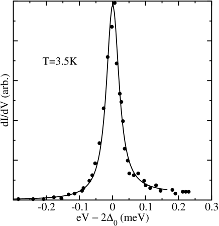
Figure 1: The calculated $dI/dV$ (solid line) and the experimental data points (filled circles) from [1] at $T$=3.5 K. The data are plotted as a function of $eV$-2$\Delta_{0}$.

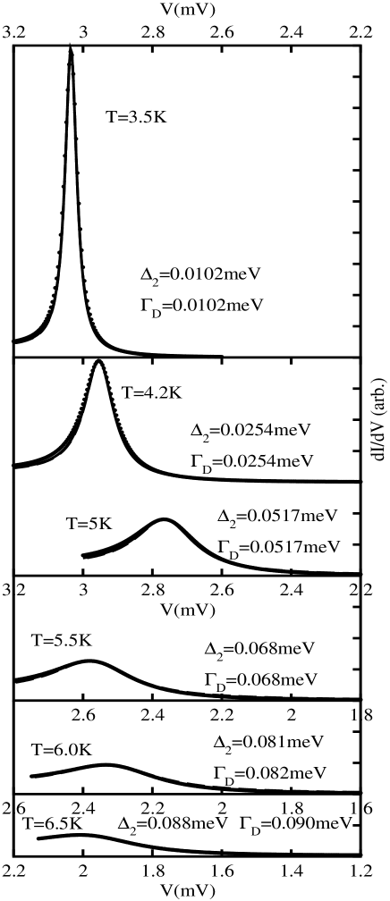
Figure 2: The calculated (filled circles) $dI/dV$ at six different temperatures as a function of voltage and their fits with (8) (solid line) and with the Dynes formula (3) (dashed line) with $\Delta_{2}$ and $\Gamma_{D}$ as the only fit parameters, respectively.

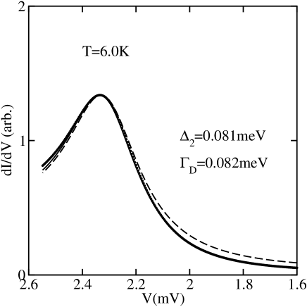
Figure 3: The calculated $dI/dV$ (dots) at T=6 K versus voltage and the fits with (8) (solid line) and (3) (dashed line), with $\Delta_{2}$ and $\Gamma_{D}$ as the only fit parameters, respectively.

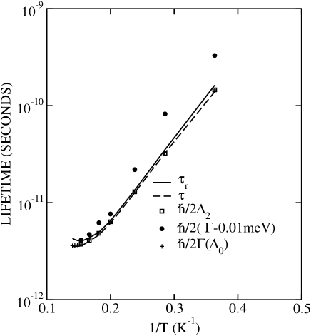
Figure 4: Quasiparticle lifetime at the gap edge determined in various ways (see the text) as a function of inverse temperature.

References

- [1] Dynes R C, Narayanamurti V, and Garno J P 1978 Phys. Rev. Lett. 41 1509
- [2] Kaplan S B, Chi C C, Langenberg D N, Chang J J, Jafarey S, and Scalapino D J 1976 Phys. Rev. B 14 4854
- [3] Dynes R C, Garno J P, Hertel G B, Orlando T P 1984 Phys. Rev. Lett. 53 2437
- [4] White A E, Dynes R C, and Garno J P 1986 Phys. Rev. B 33 3549
- [5] Review issue on MgB2, edited by Crabtree G, Kwok W, Canfield P C 2003 Physica C 385 1
- [6] Bergeal N, Dubost V, Noat Y, Sacks W, Roditchev D, Emery N, Hérold C, Marêché J-F, Lagrange P, and Loupias G 2006 Phys. Rev. Lett. 97 077003
- [7] Kurter C, Ozyuzer L, Mazur D, Zasadzinski J F, Rosenmann D, Claus H, Hinks D G, and Gray K E 2006 Preprint cond-mat/0612581
- [8] Matsui H, Hashimoto D, Souma S, Sato T, Takahashi T, and Shirotani I 2005 J. Phys. Soc. Jpn. 74 1401
- [9] Tsuda S, Yokoya T, Kiss T, Shimojima T, Shin S, Togasi T, Watanabe S, Zhang C Q, Chen C T, Sugawara H, Sato H, and Harima H 2006 J. Phys. Soc. Jpn. 75 064711
- [10] Schrieffer J R 1964 Theory of Superconductivity (New York: W A Benjamin)
- [11] Scalapino D J 1969 in Superconductivity ed R D Parks (New York: Marcel Dekker) pp 466-501
- [12] Dahm T, Hirschfeld P J, Scalapino D J, and Zhu L 2005 Phys. Rev. B 72 214512
- [13] Dynes R C and Rowell J M 1975 Phys. Rev. B 1884