The MSST Campaign: II.Effective temperature and gravity variations in the multi-periodic pulsating subdwarf B star PG1605+072^,,

Abstract

Context. Stellar oscillations are an important tool to probe the interior of a star. Subdwarf B stars are core helium burning objects, but their formation is poorly understood as neither single star nor binary evolution can fully explain their observed properties. Since 1997 an increasing number of sdB stars has been found to pulsate forming two classes of stars (the V361 Hya and V1093 Her stars).

Aims. We focus on the bright V 361 Hya star PG1605$+$072 to characterize its frequency spectrum. While most previous studies relied on light variations, we have measured radial velocity variations for as much as 20 modes. In this paper we aim at characterizing the modes from atmospheric parameter and radial velocity variations.

Methods. Time resolved spectroscopy ($\approx$9000 spectra) has been carried out to detect line profile variations from which variations of the effective temperature and gravity are extracted by means of a quantitative spectral analysis.

Results. We measured variations of effective temperatures and gravities for eight modes with semi-amplitudes ranging from $\Delta T_{\rm{eff}}=880$ K to as small as 88 K and $\Delta\log{g}$ of 0.08 dex to as low as 0.008 dex. Gravity and temperature vary almost in phase, whereas phase lags are found between temperature and radial velocity.

Conclusions. This profound analysis of a unique data set serves as sound basis for the next step towards an identification of pulsation modes. As rotation may play an important role the modelling of pulsation modes is challenging but feasible.

1 Introduction

The subluminous B stars (commonly referred to as sdBs) are generally believed to be core helium burning stars with very thin ($<$0.02 $M_{\odot}$) hydrogen envelopes which have masses around $\sim$0.5 $M_{\odot}$. Considerable evidence has accumulated that these stars are sufficiently common to be the most likely source for the “UV upturn phenomenon” observed in elliptical galaxies and spiral galaxy bulges (Yi et al. 1997). However, important questions still remain about their formation and the appropriate timescales. Following ideas outlined by Heber (1986), the sdBs can be identified with models for Extreme Horizontal Branch (EHB) stars. An EHB star bears great resemblance to a helium main-sequence star of half a solar mass and it should evolve similarly, i.e. directly to the white dwarf cooling sequence, bypassing a second giant phase.

While the next stages of sdB evolution seem to be well known, the question of the stars’ formation is widely unanswered. Nowadays evidence is growing that close binary evolution plays an important role for the formation of sdB stars (Maxted et al. 2001; Morales-Rueda et al. 2003; Napiwotzki et al. 2004).

The work of Han et al. (2003) brought remarkable progress. Three possible binary formation channels were studied: common envelope ejection, stable Roche lobe overflow and the merger of two helium white dwarfs. One of the key results of the Han et al. studies was the suggestion that the mass range of sdBs may be larger than previously thought. They found that sdB stars in binary systems may have masses as low as 0.36 $M_{\odot}$ and still pass through a helium core burning phase. Until now the mass of any sdB has always been assumed to be $\sim$0.5 $M_{\odot}$ for the determination of luminosity or binary companion mass, however now it appears this may not be entirely appropriate. What is needed is a set of precise masses that can be compared with sdB formation models such as those of Han et al.

Asteroseismology provides a promising avenue to determine masses of stars. Two classes of non-radially pulsating sdB stars have been discovered recently, the V361 Hya and V1093 Her stars (Kilkenny et al. 1997; Green et al. 2003). The V 361 Hya ones are of short period (2–8 min) and have photometric amplitudes of typically less than 10 mmag, while the V1093 Her stars have longer periods (45 to 120 min) and even smaller amplitudes of less than 2 mmag. Several of the pulsating sdB stars reside in close binary systems.

The V361 Hya stars have already been proven to be extremely useful objects for asteroseismology, because many of them show a sufficient number of modes with only small amplitude variations rendering them ideal targets for long-term photometric campaigns to resolve the frequencies of the modes in their light curves. Single site monitoring was carried out for several V 361 Hya stars. However, the complexity of the oscillations requires high frequency resolution which can only be achieved in extensive multi-site campaigns. Therefore observers have teamed up to continously collect photometry over weeks for a few V 361 Hya stars (e.g. Kilkenny et al. 1999; Silvotti et al. 2002, 2006; Randall et al. 2006).

Theoretical studies by Charpinet et al. (1997) showed that the oscillations of V361 Hya stars can be explained as acoustic modes $(p-modes)$ of low degree $l$ and low radial order $n$ excited by an opacity bump due to a local enhancement of iron-group elements. Theoretical modelling has now matured to derive stellar parameters (stellar mass and hydrogen envelope mass) by matching model predictions to the observed frequency spectra (see Charpinet et al. 2006, and reference therein).

Light variations provide important information on the oscillation properties. In order to identify the pulsation modes reliably, however, it is desirable to supplement them with measurements of stellar surface motions leading to radial velocity and line profile variations. This has been achieved for the first time for PG 1605$+$072 (O’Toole et al. 2000, see below) and attempted with diverse success for half a dozen V 361 Hya stars (Jeffery & Pollacco 2000; Woolf et al. 2002a, 2003; Telting & Østensen 2004, 2006).

PG1605$+$072 (also known as V338 Ser) was discovered by Koen et al. (1998) to be a V361 Hya and was found to have the longest periods (up to 9 min) of this class of stars and a very large photometric amplitude (up to $\sim$60 mmag). They detected a very strong main mode together with about 20 other modes. In the following years a first multi-site campaign confirmed these results and increased the number of observed frequencies up to 50 (Kilkenny et al. 1999). Using high resolution Keck spectra, the stellar parameters and metal abundances were derived by Heber et al. (1999) . They found $T_{\rm{eff}}=32,300$ K, $\log{g}=5.25$ dex and $\log{(He/H)}=-2.53$, whereas the small $\log{g}$ implies that the star is quite evolved and has already moved away from the EHB.

Radial velocity variations due to pulsation were detected for the first time by O’Toole et al. (2000) and confirmed by O’Toole et al. (2002); Woolf et al. (2002b); Falter et al. (2003). Variations of equivalent widths (line indices) were detected by O’Toole et al. (2003) and analysed for $T_{\mathrm{\rm{eff}}}$ ($\Delta T_{\mathrm{eff}}\approx 560$ K) and $\log{g}$ ($\Delta\log{g}\approx 0.062$ dex) variations. Nevertheless these studies suffered from poor frequency resolution or from the lack of simultaneous photometry. Therefore we organised a multi-site coordinated spectroscopic campaign to observe PG1605$+$072 with medium resolution spectrographs on 2 m and 4 m telescopes (MSST, Heber et al. 2003). Surface motions for more than 20 pulsation modes were detected in this data set from radial velocity variations (O’Toole et al. 2005, henceforth Paper I). In this paper we proceed to analyse the same data set for line profile variation in order to search for, analyse, and interpret variations in surface gravity and effective temperature.

The paper is organised as follows. In Sect. 2 we outline the available data and in Sect. 3 the derivation of atmospheric parameter variations by fitting model atmospheres to observed spectral lines. The phase lags between radial velocity, temperature and gravity variations are measured in Sect. 4, leading to a discussion in the last section including an outlook to the theoretical modelling of line profile variations.

2 The MSST 2m spectroscopy

During the Multi-Site Spectroscopic Telescope (MSST) campaign we obtained 151 hours of time-resolved spectroscopy on PG 1605+072 at four observatories in May/June 2002 along with extensive time-resolved photometry on 2 m class telescopes (see Heber et al. 2003). The MSST spectroscopic campaign was divided into two parts, the first of which (19–27/05/2002) was carried out at the Steward Observatory 2.3 m on Kitt Peak, the Danish 1.54 m at La Silla, and the 2.3 m Advanced Technology Telescope at Siding Spring Observatory. The second part (13–25/06/2002) took place about three weeks later, again at the Danish 1.54m at La Silla and at the 2.56 m Nordic Optical Telescope at La Palma. Details are given in Table 1 of Paper I. Spectra taken at ESO between June 13, 2002 and June 18, 2002 suffer from poor weather conditions resulting in so low S/N that they cannot be used for the spectral analysis.

Due to the different instrumentation of the observatories, the spectral resolution and coverage are quite dissimilar (see Table 1). Therefore the data sets of each telescope were analysed separately. During the first part of the campaign only three nights of observation were secured at Siding Spring Observatory and only two nights at ESO. The spectra obtained at Steward Observatory outnumber that of the former and are of much better S/N. Hence the analysis of the first part of the campaign is mainly based on the Steward data. The second part is dominated by observations from the NOT as they outnumber the ESO spectra and are of better S/N than the latter. Therefore the SSO and ESO spectra serve to check for consistency only (see Fig. 6).

Table 1: Instrumentation of the used observatories

Observatory	Resolution	$\lambda$  range	# $\mathrm{spectra}$
	(Å)	(Å)	used
MSST: first half (19/05/2002–27/05/2002):
Steward 2.3 m	1.8	3686-4534	2595
Siding Spring 2.3 m	2.2	3647-5047	852
Danish/ESO 1.54 m	5.9	3648-5147	663
second half (18/06/2002–25/06/2002):
Danish/ESO 1.54 m	5.9	3648-5147	1562
NOT 2.56 m	9.3	3039-6669	3320

The entire data set has already been analysed for radial velocity variations (Paper I) and 20 modes have been detected with radial velocity amplitudes between 0.8 and 15.4 kms ^-1. In Paper I, we calculated the spectral windows for the entire campaign as well as for the two halves. These served as a guide to the aliasing that had to be expected in the amplitude spectrum. In order to get similar primers for the Steward and NOT data sets exactly as they were used in the anaysis below, this excersise has now been repeated for the two subsets separately. Both window functions are very similar to each other, with a resolution of about 2-3 $\mu$Hz, and show the typical daily alias patters (side lobes separated by 11 $\mu$Hz) inherent to single-site observations spread over several nights. In the next step the radial velocity data set was pre-whitened in order to get rid of the main peak and aliases induced by the dominant mode.

The individual Discrete Fourier Transforms of the radial velocities with and without pre-whitening for the Steward and the NOT campaigns in the vicinity of the peak of the dominant mode are shown in Fig. 1. The amplitudes of the most important modes are given in Table 3.

Figure 1:      Fourier Transform around the mode f1 (dashed line) of the radial velocities for the Steward data (upper part) and the NOT data (lower part, mirrored). The full drawn line showes the results from pre-whitening for the strongest mode f1.

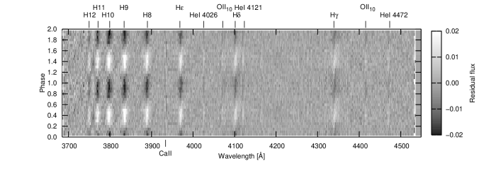
Figure 2:      Line profile variations of the phase binned Steward data for the strongest mode f1 (period P=481.74 s). The CaII line is of interstellar nature. Its variation is due to the stellar radial velocity correction. Besides the strong Balmer, He i and O ii lines are found to vary.

The one and two day alias peaks on each side of the main mode are obvious. As can be seen from Fig. 1 the amplitude of the dominant mode f1 is almost the same for both halves of the campaign.

Pre-whitening the radial velocities for the strongest mode f1 (see Fig. 1) demonstrates that the unresolved modes f2 and f3 (with a separation of 0.66 $\mu$Hz, at 2102 $\mu$Hz) are unaffected by aliases of f1. But as we are using a phase binning technique it is not obvious if this statement is also valid for the changes in the line profile.

It is evident from Fig. 1 that the radial velocity amplitude of f2,3 is much stronger in the NOT data than in the Steward data, an observation that we will come back to when discussing the results of the quantitative spectral analysis presented in the following. The same is true for the mode f4, which is situated in an area of the frequency spectrum where no aliasing effects of the dominant mode are expected (see Table 3).

As individual spectra are too noisy for a quantitative spectral analysis in terms of detecting very small variations, they were combined in an appropriate way. For each spectrum the Doppler shift produced by the star itself and the heliocentric correction was removed. The required values for each single spectrum have already been determined and used in Paper I. After that a continuum was fitted to the spectrum and a dispersion correction was applied. To be able to detect tiny variations for any pre-chosen pulsation mode, we determined the phase of each individual spectrum (with respect to the same ephemeris zero point $t_{0}(HJD)=2452413.27166681$) according to the selected pulsation period and co-added them accordingly. To this end a complete pulsation cycle was divided into twenty phase bins. In order to achieve the best possible result, we include a weighting procedure, in which every single spectrum is co-added according to its signal-to-noise-ratio. The quality of the co-added spectra improved significantly. In Fig. 2 the phase dependent changes in the line profiles of the Steward data with respect to the mean spectrum are shown. It is evident that all the observed H, He i and O ii lines vary in the same way with phase. Unfortunately there are no He ii lines present in the spectral range of the data from the Steward observatory. The Nordic Optical Telescope does give a broader wavelength coverage at much lower spectral resolution. Fig. 3 displays a section of the NOT spectra covering He ii 4686 Å along with He i 4471 Å and three Balmer lines. Unfortunately the spectral resolution is not high enough to clearly detect the He i 4471 Å , but the Balmer lines show the same behaviour (see Fig. 2). As expected the variations of the He ii line are anti-correlated with those for the Balmer lines.

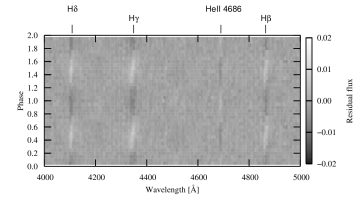
Figure 3:      Line profile variations of the phase binned NOT spectra for the strongest mode f1 (period P=481.74 s). Note the presence of He ii 4686 Åvarying in antiphase with the Balmer lines.

3 Quantitative spectral analysis and atmospheric parameter variations

Effective temperatures ($T_{\rm eff}$), surface gravities ($\log{g}$), and helium abundances ($y=N_{\mathrm{He}}/N_{\mathrm{H}}$) were determined by fitting synthetic model spectra to all hydrogen and helium lines simultaneously, using a procedure developed by Napiwotzki et al. (1999). A grid of metal line-blanketed LTE model atmospheres with solar metal abundance (Heber et al. 2000a) as well as a grid of partially line-blanketed NLTE model atmospheres (Napiwotzki 1997) was used. LTE and NLTE atmospheric parameters differ slightly due to systematic differences between these model grids.

We derived the mean effective temperatures, gravities and helium abundances for each of the four data set (see Table 2) as will be described in section 3.1 . When comparing the results one must take into account that not only the spectra are of different resolution but that also different sets of spectral lines had to be used due to limitations by different wavelengths coverages. As can seen from Table 2 the formal statistical fitting errors are less than 70 K, 0.015 dex and 0.020 dex, respectively. As the differences between the results from different data sets and different model grids are much larger, we conclude that the formal errors are unrealistically small and the error budget is dominated by systematic errors both from observations as well as from model atmospheres. More realistic error estimates are 500 K for $T_{\rm eff}$, 0.05 dex for $log\,g$, and 0.1 dex for $log\,N(He)/N(H)$ (for a more detailed discussion see Heber et al. 2000b; O’Toole & Heber 2006; Geier et al. 2007). Within these limits the results from the Steward, the NOT and the SSO data sets agree very well with each other as well as with the result of Heber et al. (1999). The ESO spectra, however, give significantly lower temperatures. However, the variation of the atmospheric parameters can be determined with much higher precision than their absolute values as the systematic errors cancel to a very large extend in a strictly differential analysis.
In Fig. 4 a fit of the Steward spectrum for one phase bin (weighted sum of more than 100 individual spectra) is displayed.

We are now prepared to search for and analyse variations of the atmospheric parameters, effective temperatures, surface gravities, and helium abundances ($y=N_{\mathrm{He}}/N_{\mathrm{H}}$). As the dominant mode in radial velocity is expected to also show the largest variation in temperature and gravity, we start with this mode and repeat the procedure for weaker modes.

Note that the apparent variations of the atmospheric parameters are disk intergrated. The actual amplitudes at different positions on the stellar surface can be considerably larger depending on the type of mode. For a radial one disk-intergrated values should differ only slightly from the actual values on the surface. But for non-radial modes the importance of cancellation effects grows with rising degree l.

Figure 4:      Fit of the observed H/He lines from a Steward spectrum. The $\mathrm{H}_{\epsilon}$ core is affected by the interstellar Ca ii, H line.

3.1 The strongest mode

In the first step we considered the mode with the largest radial velocity amplitude and stacked the individual spectra accordingly into 20 phase bins. We determined the variations of the three atmospheric parameters ($T_{\rm{eff}}$, $\log{g}$ and $\log{He/H}$-ratio) for every bin. Fig. 5 shows the variations of the atmospheric parameters for the Steward Observatory data. As can be seen the variations of $T_{\rm{eff}}$ and $\log{g}$ are sinusoidal. Therefore the pulsation semi-amplitude is determined by using a $\chi^{2}$ sine fitting procedure.

Figure 5:      The variations of the atmospheric parameters determined from the Steward data with statistical error bars and sine fit are shown.
Upper panels: temperature and surface gravity with sine fits are shown.
Lower panels: He/H abundance and the temperature residuals (with a sine fit for the first harmonic) are shown.

The temperature semi-amplitude is $874\,\mathrm{K}$, while the surface gravity variation is $\pm 0.078\,\mathrm{dex}$. We also plotted the He/H abundance to make sure that it does not show periodical variations over a cycle. The remaining temperature residuals still show a periodicity (of $\pm 72\,\mathrm{K}$) with frequency f10 which was also already identified as the first harmonic in Paper I. As expected the amplitude ratio between the RVs (15.43 $\mathrm{kms^{-1}}$: 1.36 $\mathrm{kms^{-1}}$= 11.3) is similar to the ratio of the temperature amplitudes (873.7 K : 72.0 K = 12.1). Analogue we succeded to detect the first harmonic also in the $\log{g}$ residuals with an amplitude of $\pm 0.013\,\mathrm{dex}$, whereas the amplitude ratio is significant lower (0.078 dex : 0.013 dex = 6.0).

Fig. 6 compares the temperature and gravity variations of the strongest mode f1 derived from all four data sets. The semi-amplitudes, derived from a sine fit as well, are consistent within error limits (see Table 2), except for the gravity amplitudes in the ESO spectra. This is hard to explain as the ESO observations overlap in time with those at the NOT. We conjecture that this is due to the limited number and lower quality of the ESO spectra.

Observatory	$\overline{T_{\rm eff}}$ [K]	$\overline{\log{g}}$ [dex]	$\overline{\log{n_{\rm{He}}/n_{\rm{H}}}}$ [dex]	$\Delta T_{\rm eff}$ [K]	$\Delta\log{g}$ [dex]
Steward	31999.9$\pm$17.3	5.262$\pm$0.004	-2.59$\pm$0.005	873.7$\pm$16.5	0.078$\pm$0.003
NOT	31927.9$\pm$27.1	5.299$\pm$0.004	-2.58$\pm$0.007	840.9$\pm$26.0	0.079$\pm$0.004
SSO	32426.8$\pm$67.7	5.260$\pm$0.011	-2.46$\pm$0.015	808.9$\pm$64.9	0.082$\pm$0.010
ESO	31437.7$\pm$31.5	5.224$\pm$0.008	-2.58$\pm$0.011	793.7$\pm$30.2	0.054$\pm$0.008

Table 2: The dominant mode f1: comparison of temperature and surface gravity mean values and semi-amplitudes from different data sets.

As the variations with phase of the atmospheric parameters for the dominant mode f1 have been measured in all data sets beyond doubt, we proceeded to search for and analyse weaker modes. We re-binned all spectra according to their phases with respect to the frequency of a weaker mode and proceeded with all modes with decreasing radial velocity amplitude (f2, f3 and so on). For these three modes with lower amplitudes (f2-f4) periodic variations of the atmospheric parameters were found in both the Steward and the NOT data set. As a test we applied the procedure to a random frequency not detected in velocity or light. Periodic variation of the atmospheric parameters were found neither in the Steward nor in the NOT data indicating that the dominant mode produces sufficient self-cancellation for its influence to be annihilated.

Figure 6:      Temperature and log g variations of the dominant mode f1 from all available data sets; from top to bottom: NOT($\square$), Steward(x), SSO(+) and the ESO($\divideontimes)$. For clarity, the curves have been offset by 750 K in $T_{\rm eff}$ and 0.1 dex in gravity. The best fit sine curves are the dotted (NOT), full drawn (Steward), short dashed (SSO) and dashed (ESO) lines.

3.2 Cleaning the spectra

As is clearly seen from Fig. 1, the main mode produces alias peaks close to the location of f2 and f3. For f4 onwards the influence is much smaller, but due to the high amplitude of the main mode the influence can still be significant. Unlike the case for the photometry and radial velocity data, which can be cleaned using a standard pre-whitening procedure, a more sophisticated approach is required to remove the influence of the main mode from the spectroscopic data. Hence we have implemented a cleaning procedure based on our synthetic model spectra.

First we calculated synthetic spectra for every phase bin of the dominant pulsation mode f1. Then they were summed up to create the mean synthetic spectrum for f1, which was subtracted from each phase bin spectrum to form the cleaning function. This correction was applied to all of the $\sim 9000$ individual spectra by subtracting the cleaning function for the corresponding phase of the dominant mode. The cleaned spectra were then summed into 20 phase bins for the corresponding frequencies of lower amplitude modes (from f2 onwards) and were analysed for the atmospheric parameter variations as described above. As a test we applied the procedure to the dominant mode f1 as well. The residual amplitudes are listed in Table 3 and shown in Fig. 7. As can be seen, no significant residuals remain for the NOT data, while small residuals remain in particular in the Steward spectra, which may be basically due to the 1st harmonic mode f10 (see section 3.1) and the limitations of the model spectra as we assume e.g. a homogenous temperature distribution on the surface.

Name	Period	f	v	$\Delta T_{\rm eff}$	$\Delta T_{\rm eff}$	$\Delta\log{g}$	$\Delta\log{g}$
	(s)	($\mu$Hz)	$kms^{-1}$	(K)	(K)	(dex)	(dex)
				no cleaning	cleaning	no cleaning	cleaning
Steward Observatory
f1	481.74	2075.80	15.429	873.7$\pm$16.5	70.5$\pm$4.7	0.078$\pm$0.003	0.008$\pm$0.001
f2	475.61	2102.55	5.372	218.5$\pm$15.3	132.6$\pm$12.6	0.019$\pm$0.002	0.011$\pm$0.002
f3	475.76	2101.91	2.971	209.1$\pm$18.3	84.5$\pm$17.5	0.019$\pm$0.002	0.008$\pm$0.002
f4	364.56	2743.01	2.497	141.8$\pm$11.2	140.9$\pm$14.6	0.011$\pm$0.002	0.011$\pm$0.002
f5	503.55	1985.89	2.474	-	117.9$\pm$10.3	-	0.014$\pm$0.002
f6	528.71	1891.41	2.322	-	87.7$\pm$15.0	-	0.009$\pm$0.002
f7	361.86	2763.50	2.121	-	136.8$\pm$10.5	-	0.013$\pm$0.003
f8	246.20	4061.70	1.777	-	88.1$\pm$18.3	-	0.021$\pm$0.002
NOT Observatory
f1	481.74	2075.80	15.429	840.9$\pm$26.0	18.9$\pm$21.3	0.079$\pm$0.004	0.000$\pm$0.003
f2	475.61	2102.55	5.372	212.6$\pm$31.9	218.4$\pm$28.3	0.024$\pm$0.003	0.018$\pm$0.003
f3	475.76	2101.91	2.971	300.3$\pm$24.4	219.5$\pm$18.3	0.031$\pm$0.003	0.018$\pm$0.002
f4	364.56	2743.01	2.497	194.5$\pm$19.8	215.8$\pm$27.1	0.024$\pm$0.003	0.031$\pm$0.004

Table 3: Semi-amplitudes of the temperature and gravity variations before and after cleaning for the four strongest modes derived from Steward and NOT data. Also the statistical error from the $\chi^{2}$ sine fitting is listed. Periods, frequencies and radial velocity amplitudes are taken from Paper I and therefore calculated for the whole MSST data run.

Figure 7:      left hand side: Steward spectra: variations of the temperature (top) and the log g (bottom) for the four strongest modes before (+) and after (x) the cleaning procedure with the statistical error bars. The best fit sine curves are the full drawn (without the cleaning) and dashed (after the cleaning) lines.
     right hand side: same for the NOT spectra.

An important improvement achieved by the cleaning is that the statistical errors of the individual atmospheric parameters derived for each phase bin decrease by a factor of 2, allowing the detection of even weaker variations in temperature ($\sim 80\rm{K}$) and gravity ($\sim 0.01\rm{dex}$), as demonstrated below.

The amplitudes of the atmospheric parameter variation for f4 are unaffected by the cleaning procedure. However the amplitudes derived from the Steward data are significantly lower than those from the NOT data. This is consistent with the lower RV amplitude in the Steward data (see Sect. 2).

Unlike f4, the amplitudes for f2 and f3 of the Steward data decreased after cleaning. The same holds for f3 in the NOT data, while f2 is almost unaffected by cleaning. Note that f2 and f3 are so close in frequency that they are not resolved in either data set.

At this point we would like to refer again to Fig.1; the amplitude in radial velocity for f2,3 is much higher in the NOT data than in the Steward data set and the same holds for f4. The differences in the detected temperature and gravity variations between the Steward and the NOT data sets are consistent with the radial velocity amplitudes and therefore plausible.

3.3 The weak pulsations f5–f11

Without the cleaning we were able to detect temperature and gravity variations only for those four frequencies with the largest radial velocity amplitudes. Since the statistical errors of atmospheric parameters are significantly reduced by the cleaning procedure, it is worthwhile to search for additional frequencies. The Steward spectra are suited best because they have the highest spectral resolution, S/N, and the second largest number of spectra. Indeed, we detected weaker modes (see Fig.8). The semi-amplitudes determined again by $\chi^{2}$ fitting of a sine function are listed in Table 3. For the mode f9 the errors of our data points ($\delta T_{\rm eff}=40\,\rm{K},\delta\log{g}=0.008\,\rm{dex}$) are of the same order of magnitude as the amplitude ($\Delta T_{\rm eff}=35\,\rm{K},\Delta\log{g}=0.003\,\rm{dex}$) and the detection of variations must be regarded as marginal.
Nevertheless, this demonstrates that it is possible to reveal variations of atmospheric parameters of modes with radial velocity variations down to 2 $\mathrm{kms^{-1}}$.

Frequencies f5 and f6 are isolated and therefore well resolved. Temperature variations are found at amplitudes of 110 K and 90 K, respectively while gravity variations of 0.014 dex and 0.008 dex are detected.

Frequencies f7, f9, and f11 are close together and therefore unresolved. While amplitude variations of atmospheric parameters are found for f7, the variations for f9 and f11 are below the detection limit.

f8 and f10 are combination frequencies involving f1 (f1+f5 and 2$\times$f1, respectively). For f8 the variation of $T_{\mathrm{eff}}$ is detected marginally only, whereas the gravity variation is pronounced (see Fig.8 and Table 3). f10 was already detected in the residuals of the sine fit to f1 as discussed in Section 3.1 (see also Fig. 5).

Figure 8:      Variations of the temperature(left) and the log g(right) for the modes f5, f6, f7 and f8 after the cleaning procedure with sine fits and statistical error bars derived for the Steward data.

4 Phase lags

In order to characterise pulsation modes it is important to investigate phase lags between temperature, gravity and radial velocity variations as well. These phase lags can be used to determine the deviations from a linear adiabatic system.

4.1 Temperature versus radial velocity

The radial velocities of individual spectra were taken from Paper I. The amplitudes of their variations were determined in the same way as the temperature and gravity variations using the phase binning technique and cleaning described in Sect 2. Phase lags between the variation of radial velocity and temperature can be derived directly by comparing the phases of the maxima of the $T_{\rm eff}$ and RV curves.

	Steward				NOT
	$\Delta\varphi(T_{\rm{eff}}-RV)$	$\Delta\varphi(T_{\rm{eff}}-\log{g})$		$\Delta\varphi(\log{g}-RV)$	$\Delta\varphi(T_{\rm{eff}}-RV)$	$\Delta\varphi(T_{\rm{eff}}-\log{g})$		$\Delta\varphi(\log{g}-RV)$
Name	cleaning	no cleaning	cleaning	cleaning	cleaning	no cleaning	cleaning	cleaning
f1	+0.293	+0.040	-	+0.253	+0.311	+0.039	-	+0.272
f2	+0.289	+0.054	+0.054	+0.235	+0.351	+0.054	+0.053	+0.300
f3	-0.131	+0.063	+0.193	-0.275	+0.184	+0.019	+0.031	+0.153
f4	+0.260	-0.016	-0.011	+0.271	+0.280	-0.007	+0.007	+0.298
f5	+0.268	-	+0.034	+0.234	-	-	-	-
f6	+0.219	-	-0.013	+0.231	-	-	-	-
f7	+0.364	-	-0.006	+0.370	-	-	-	-
f8	+0.238	-	+0.048	+0.182	-	-	-	-

Table 4: Phase lags $\Delta\varphi$ (in units of $2\pi$) between $T_{\rm eff}$, radial velocity and $\log{g}$ derived from the Steward and NOT data before and after the cleaning. Positive values mean that the maximum of the radial velocity or gravity curve occurs before that of $T_{\rm eff}$ or $\log{g}$. The values for the radial velocities are taken from Paper I.

The phase lag between the temperature and the radial velocity variation for the dominant mode is displayed in Fig. 9.

Figure 9:      Radial velocity (x) and the temperature variation (+) of the dominant mode f1 derived from the Steward data. The dashed line is the best fit sine curve for the $T_{\rm eff}$ variations; the dotted line is the best sine curve for the radial velocity variation.

In order to determine the phase lags of the weaker modes we used the temperature curves after cleaning. We just measure the phase lags for two sine functions. The formal fitting errors are unrealistically small. Systematic errors are probably more important but hard to quantify. As we have two independant measurements at hand (Steward, NOT) we can use them to estimate the error. As f2/f3 are not suitable due to blending, we obtain an error estimate of $\pm 0.025$ from f1 and f4.

The results for all the recovered modes are shown in Table 4.

It is worth noting that for all recovered modes exept f3 the radial velocity variation reaches its maximum before the temperature variation which means throughout positive values for the phase lags. Furthermore, all the values of the phase lags lie around $0.25$($\triangleq\frac{\pi}{2}$) with small but significant deviations. This is the value we would expect for a completely adiabatic p-mode pulsation. But as a real star is a non-adiabatic system due to its radiation of light, such deviations are to be expected (see Table 4).

For the dominant mode f1 the phase lag between $T_{\rm{eff}}$ and $log{g}$ is 0.3 (see Table 4) indicating that the temperature is highest shortly after the radius is smallest.

At this point we would like to emphasise our results for f3. Comparing the temperature variation plots for f3 in Figure 7 it is obvious that the phase of the two sine functions without cleaning differs by a value of $0.5$ ($\triangleq\pi$) in phase between the Steward and the NOT results. At the same time, the phases of the radial velocity curves between the two main data sets differ by about $0.25$ ($\triangleq\frac{\pi}{2}$). After the cleaning the situation does not improve much, as we still meausure a phase lag of $+0.315$ for temperature and $+0.428$ for gravity between the Steward and the NOT data.

If real, this would indicate that a phase jump occurred between the two observing runs. However since f3 is unresolved from f2 (see Fig. 1) this phenomenon could well be an artifact. It is quite unfortunate that we could not combine Steward and NOT data in the quantitative analysis, because the 38 days coverage should have given us the required time resolution.

4.2 Temperature versus gravity

As before the phase lags between the variation of temperature and gravity can be derived directly by comparing the phases of the maxima of the $T_{\rm eff}$ and $\log{g}$ curves. In Table 4 we give the phase lags with and without cleaning. The result is that the phase lags between $T_{\rm eff}$ and $\log{g}$ are rather small.

The phase lags between $T_{\rm eff}$ and $\log{g}$ are insensitive to the cleaning procedure for f2. Within the maximum error limits of half the bin size (i.e. 0.025) the phase lags found in the Steward spectra are consistent with those from NOT spectra.

For f3 the situation is very different as the phase lags show a rather large discrepancy between the two data sets. Referring again to Fig.1 and Fig.7 it is obvious that the mode f3 seems to change in both, phase and amplitude between the two parts of the campaign. Another point is that the peak of the unresolved modes f2/f3 is much higher in the NOT data than in the Steward data. If we take also into account the detection of a much higher amplitude in $T_{\rm eff}$ and $\log{g}$ for f3 after the cleaning (see Table 3 and Fig.7), it is more likely that the phase lag for f3 from the NOT data constitute a more reliable measurement in this case.

4.3 Radial velocity versus gravity

Finally, we consider the phase lags between the radial velocity and the gravity. As they are both produced by the movement of the stellar surface, they are supposed to have a strict relationship. I.e. the g variation should be inline with the derivative of the radial velocity curve. Hence we expect a phase lag of $\frac{\pi}{2}$ between the RV curve and the $\log{g}$ curve.

We apply the same fitting procedure as before. The results are shown in Table 4.

Alternatively we can calculate $\Delta\varphi(\log{g}-RV)$ from $\Delta\varphi(T_{\rm{eff}}-RV)-\Delta\varphi(T_{\rm{eff}}-\log{g})$. The small difference between the two methods indicates the consistancy of our measurements.

For the Steward data most values seem to be in agreement with the theory within 0.02 consistent with our error estimate in Sect. 4.1, except for frequencies f3, f7 and f8. The difficulty with f3 have already been discussed (see above) and the same may hold for f7 as it also unresolved from f9, wereas frequency f8 is close to the detection limit (see Sect.3). While the phase lags $\Delta\varphi(\log{g}-RV)$ are consistent with expectation (0.25) the phase lags from NOT data show a systematic offset of $\sim 0.04$. Overall the phase lags from Steward data appear to be more reliable.

5 Discussion

The quantitative spectral analysis of about 9000 spectra of the pulsating subdwarf B star PG 1605+072 obtained in the context of the MSST campaign allowed us to detect line profile variations of those four modes that show the strongest radial velocity variations, as well as for the first harmonic of the dominant mode. The data set was obtained at four observatories in two observing periods in May 2002 and June 2002 separated by about three weeks. Spectra of the first half were predominantly taken at the Steward 2.3m telescope at KPNO, while those of the second half were mostly from the Nordic Optical Telescope. Spectra taken at the Siding spring observatory and at ESO were used for a consistency check only.

Using a new cleaning technique we obtained more precise results, which allowed us to detect tiny line profile variations for four additional modes, including a combination frquency, with radial velocity variation as small as 1.8 $\mathrm{kms^{-1}}$. Variations of the effective temperature and gravity are sinusoidal and with semi-amplitudes ranging from 90 K to 870 K in effective temperature and from 0.009 dex to 0.078 dex in gravity. We find evidence for amplitude variations between the first and the second half of the MSST campaign for f2/f3 and the f4 mode but not for f1. As f2/f3 are unresolved this could be due to beating. The analysis of the contemporary MSST photometry indicates that f4 could actually be split in two modes (Schuh et al., 2007 in prep.) and the amplitude changes found could be as well caused by beating (Paper III).

We also measured the phase shift between the temperature, the gravity and the radial velocity curves. Effective temperature and gravity show only a small phase lag. This is not the case for the phase shifts between radial velocity and temperature. All phase shifts except for f3 in the Steward data lie around $\frac{\pi}{2}$ (between 0.20 and 0.30 in units of $2\pi$), which is expected for adiabatic pulsations, while f7 shows a somewhat larger phase of 0.37. Most notably, however, for the dominant mode the maximum of the star’s temperature occurs shortly after the minimal radius.

Kuassivi et al. (2005) measured radial velocity and flux variations from far-UV time-resolved spectroscopy and determined a phase shift of $\pi$ between the maxima of radius and flux of the strongest mode. As the flux variation is mainly caused by temperature variations and maximum radius occurs at zero velocity, this translates into a phase shift of $\pi/2$ between the temperature and radial velocity variations, in agreement with our results.

The behaviour of the mode f3 poses problems. The amplitudes as well as the phasing of the temperature, gravity and radial velocity variations are sensitive to the cleaning procedure. Moreover, there seems to be a phase jump between the two halves of the observing campaigns unlike for any other mode. Phase variations have been observed in the V361 Hya star HS 1824+5745 (Reed et al. 2006) but remained unexplained. However, as the frequency of f3 is very close to that of f2 they are unresolved at least in terms of radial velocity. f3 may be strongly influenced by f2, which renders our results for f3 dubious.

Variations of the atmospheric parameters have already been derived by O’Toole et al. (2003) from variations of Balmer line indices. The measurements were based on time resolved spectroscopy carried out in 1999 and 2000. The same grid of model atmospheres as used here was employed to derive effective temperatures and gravities from Balmer line indices. Unlike in this paper, effective temperature and gravities were determined independantly. After measuring T_eff with a fixed gravity, the adopted gravities were determined keeping T_eff fixed.

The radial velocity amplitudes of individual modes change dramatically from year to year. The radial velocity variations of the dominant mode f1 at 2075 $\mu$Hz during the MSST campaign for instance increase from 2.4 $\mathrm{kms^{-1}}$ in 1999 to 4.27 $\mathrm{kms^{-1}}$ in 2000 to 15.4 $\mathrm{kms^{-1}}$ in 2002. Therefore it might be misleading to compare the amplitudes of temperature and gravity variations at different epochs. We would expect the temperature and gravity variations to scale with the amplitude of the radial velocity curve, which is indeed evident. The T_eff/$\log{g}$ variations for 1999 and 2000 are much smaller than in 2002 as were the RV amplitudes (O’Toole et al. 2000).

Telting & Østensen (2004) were the first to derive temperature and gravity variation for a pulsating sdB star from fitting synthetic line profiles to time-series spectroscopy. They detected line profile variations in PG 1325$+$101 and derived temperature and gravity variation for the dominant mode using the same grid of model atmospheres as used here. The amplitudes of the radial velocity, T_eff and $\log{g}$ for PG 1325$+$101 (12.3 $\mathrm{kms^{-1}}$, 610 K, 0.051 dex, respectively) are somewhat smaller than for PG 1605$+$072 (15.4 $\mathrm{kms^{-1}}$, 857 K, 0.079 dex). Moreover, Telting & Østensen (2004) measured phase lags between temperature, gravity and radial velocity for PG 1325$+$101 and found exactly the same values as we do for PG 1605$+$072 ($\Delta\phi$(T${}_{\rm eff}-RV$)=+0.29 and $\Delta\phi$(T${}_{\rm eff}-\log{g}$)=+0.04).

Telting & Østensen (2004) assumed that the dominant mode in PG 1325$+$101 is a radial one and calculated the amplitude of the radius variation and the amplitude of the pulsational acceleration. We apply the same procedure to PG 1605$+$072 and find that the variation of the radius is 0.9% and the pulsational acceleration is 0.292 kms^-2 corresponding to variations of surface gravity by $\Delta\log{g}$ = 0.008 dex and 0.072 dex, respectively. As in the case of PG 1325$+$101 the pulsational acceleration is far more important than the change in radius. The predicted change in gravity is remarkably close to the measured value (0.078 dex). However, we are reluctant to conclude that f1 is a radial mode, because the temperature variations have to be matched as well, which needs further detailed modelling.

The MSST campaign has also obtained an unprecedented set of time resolved photometry, which will be presented and analysed in a forthcoming Paper III. A small part of the MSST photometry has been used by Pereira & Lopes (2005) to demonstrate that there is no stochastic mechanism exciting the oscillations in the subdwarf B star PG 1605+072. The full set of observations (radial velocity curve from Paper I, temperature and gravity variations from this paper and the light curve analyses) will then form a sound basis for astroseismology.

For this purpose the modes have to be classified first, i.e. the pulsational ”quantum” numbers have to be determined. This needs appropriate modelling. Sophisticated linear, adiabatic and non-adiabatic models for non-radial pulsations are available and have been successfully applied to match model prediction to the the observed periods from light curve analysis (see e.g. Charpinet et al. 2006). The case of PG 1605$+$072 is more complicated because rotation may play an important role. Kawaler (1999) suggested a model that fitted the five strongest modes if the star rotates rapidly at 130 $\mathrm{kms^{-1}}$. Heber et al. (1999) backed this up by measuring line broadening of 39 $\mathrm{kms^{-1}}$and interpreted this as the projected rotational velocity assuming that broadening due to pulsational motions are negligible. Since it is now clear that pulsational motions add significantly to the line broadening, the projected rotational velocity is smaller than anticipated.

Nevertheless, pulsational models have to account for rotation as well. A numerical code to model line profile variations due to adiabatic non-radial pulsations for rapidly rotating early type stars has been developed by Townsend (1997) and successfully applied to explain the pulsations of Be stars (Rivinius et al. 2003; Maintz et al. 2003). This code, named BRUCE, is well suited to model the pulsations of PG 1605$+$072 as well. It has already been used to calculate synthetic photometry for non-radial pulsations in subdwarf B stars by Ramachandran et al. (2004). We shall apply this approach to model the light curve, the radial velocity curve as well as the temperature/gravity variations of PG1605+072 in a forthcoming paper (Paper IV).