Explicit Formula for Constructing Binomial Confidence Interval with Guaranteed Coverage Probability

Abstract.

In this paper, we derive an explicit formula for constructing the confidence interval of binomial parameter with guaranteed coverage probability. The formula overcomes the limitation of normal approximation which is asymptotic in nature and thus inevitably introduce unknown errors in applications. Moreover, the formula is very tight in comparison with classic Clopper-Pearson’s approach from the perspective of interval width. Based on the rigorous formula, we also obtain approximate formulas with excellent performance of coverage probability.

1. Classic Confidence Intervals

The construction of confidence interval of binomial parameter is frequently encountered in communications and many other areas of science and engineering. Clopper and Pearson [3] has provided a rigorous approach for constructing confidence interval. However, the computational complexity involved with this approach is very high. The standard technique is to use normal approximation which is not accurate for rare events, especially in the context of studying the bit error rate of communication systems, blocking probability of communication networks and probability of instability of uncertain dynamic systems. Moreover, it has been recently proven by Brown, Cai and DasGupta [1, 2] that the standard normal approximation approach is persistently poor. The coverage probability of the confidence interval can be significantly below the specified confidence level even for very large sample sizes. Since in many situations, it is desirable to quickly construct a confidence interval with guaranteed coverage probability, our goal is to derive a simple and rigorous formula for confidence interval construction.

Let the probability space be denoted as $(\Omega,F,P)$ where $\Omega,F,P$ are the sample space, the algebra of events and the probability measure respectively. Let $X$ be a Bernoulli random variable with distribution ${\rm Pr}\{X=1\}=\mathbb{P}_{X},\;\;{\rm Pr}\{X=0\}=1-\mathbb{P}_{X}$ where $\mathbb{P}_{X}\in(0,1)$. Let the sample size $N$ and confidence parameter $\delta\in(0,1)$ be fixed. We refer an observation with value 1 as a successful trial. Let $K$ denote the number of successful trials during the $N$ i.i.d. sampling experiments. Let $k=K(\omega)$ where $\omega$ is a sample point in the sample space $\Omega$.

1.1. Clopper-Pearson Confidence Limits

The classic Clopper-Pearson lower confidence limit $L_{N,k,\delta}$ and upper confidence limit $U_{N,k,\delta}$ are given respectively by

$$L_{N,k,\delta}\stackrel{{\scriptstyle\mathrm{def}}}{{=}}\left\{\begin{array}[]{ll}0&{\rm if}\;k=0\\ \underline{p}&{\rm if}\;k>0\end{array}\right.\;\;\;{\rm and}\;\;\;U_{N,k,\delta}\stackrel{{\scriptstyle\mathrm{def}}}{{=}}\left\{\begin{array}[]{ll}1&{\rm if}\;k=N\\ \overline{p}&{\rm if}\;k<N\end{array}\right.$$

where $\underline{p}\in(0,1)$ is the solution of the following equation

(1.1) $$\sum_{j=0}^{k-1}{N\choose j}\underline{p}^{j}(1-\underline{p})^{N-j}=1-\frac{\delta}{2}$$

and $\overline{p}\in(0,1)$ is the solution of the following equation

(1.2) $$\sum_{j=0}^{k}{N\choose j}\overline{p}^{j}(1-\overline{p})^{N-j}=\frac{\delta}{2}.$$

The probabilistic implication of the confidence limits can be illustrated as follows: Define random variable $L:\Omega\rightarrow[0,1]$ by $L(\omega)=L_{N,K(\omega),\delta}\;\;\forall\omega\in\Omega$ and random variable $U:\Omega\rightarrow[0,1]$ by $U(\omega)=U_{N,K(\omega),\delta}\;\;\forall\omega\in\Omega$. Then

$${\rm Pr}\{L\leq\mathbb{P}_{X}\leq U\}>1-\delta.$$

The exact value of ${\rm Pr}\{L\leq\mathbb{P}_{X}\leq U\}$ is referred as the coverage probability. Accordingly, we refer ${\rm Pr}\{\mathbb{P}_{X}<L\;{\rm or}\;\mathbb{P}_{X}>U\}$ as the error probability.

1.2. Normal Approximation

It is easy to see that the equations (1.1) and (1.2) are very hard to solve and thus the confidence limits are very difficult to determine using Clopper-Pearson’s approach. For large sample size, it is computationally prohibitive. To get around the difficulty, normal approximation has been widely used to develop simple approximate formulas (see, for example, [1, 2, 5, 6] and the references therein ). The basis of the normal approximation is the Central Limit Theorem, i.e.,

$$\lim_{N\rightarrow\infty}\Pr\left\{\frac{\left|\frac{K}{N}-\mathbb{P}_{X}\right|}{\sqrt{\frac{\mathbb{P}_{X}(1-\mathbb{P}_{X})}{N}}}<z\right\}=2\Phi(z)-1$$

where $z>0$ and $\Phi(.)$ is the normal distribution function. Let $Z_{\frac{\delta}{2}}$ be the critical value such that $\Phi(Z_{\frac{\delta}{2}})=1-\frac{\delta}{2}$. It follows that

$$\lim_{N\rightarrow\infty}\Pr\left\{\frac{K}{N}-Z_{\frac{\delta}{2}}\sqrt{\frac{\mathbb{P}_{X}(1-\mathbb{P}_{X})}{N}}<\mathbb{P}_{X}<\frac{K}{N}+Z_{\frac{\delta}{2}}\sqrt{\frac{\mathbb{P}_{X}(1-\mathbb{P}_{X})}{N}}\right\}=1-\delta,$$

i.e.,

$\lim_{N\rightarrow\infty}\;\Pr\left\{\frac{\frac{K}{N}+\frac{Z_{\frac{\delta}{2}}^{2}}{2N}-Z_{\frac{\delta}{2}}\sqrt{\frac{\frac{K}{N}(1-\frac{K}{N})}{N}+\frac{Z_{\frac{\delta}{2}}^{2}}{4N^{2}}}}{1+\frac{Z_{\frac{\delta}{2}}^{2}}{N}}<\mathbb{P}_{X}<\frac{\frac{K}{N}+\frac{Z_{\frac{\delta}{2}}^{2}}{2N}+Z_{\frac{\delta}{2}}\sqrt{\frac{\frac{K}{N}(1-\frac{K}{N})}{N}+\frac{Z_{\frac{\delta}{2}}^{2}}{4N^{2}}}}{1+\frac{Z_{\frac{\delta}{2}}^{2}}{N}}\right\}=1-\delta$.

Since $\frac{Z_{\frac{\delta}{2}}^{2}}{N}\approx 0$ for sufficiently large sample size $N$, the lower and upper confidence limits can be estimated respectively as

$$\widetilde{L}\approx\frac{k}{N}-Z_{\frac{\delta}{2}}\sqrt{\frac{\frac{k}{N}(1-\frac{k}{N})}{N}}$$

and

$$\widetilde{U}\approx\frac{k}{N}+Z_{\frac{\delta}{2}}\sqrt{\frac{\frac{k}{N}(1-\frac{k}{N})}{N}}.$$

The critical problem with the normal approximation is that it is of asymptotic nature. It is not clear how large the sample size is sufficient for the approximation error to be negligible. Such an asymptotic approach is not good enough for many practical applications involving rare events.

2. Rigorous Formula

It is desirable to have a simple formula which is rigorous and very tight for the confidence interval construction. We now propose the following simple formula for constructing the confidence limits.

Theorem 1.

Define

(2.1) $$\mathcal{L}(k)\stackrel{{\scriptstyle\mathrm{def}}}{{=}}\frac{k}{N}+\frac{3}{4}\;\frac{1-\frac{2k}{N}-\sqrt{1+4\theta\;k(1-\frac{k}{N})}}{1+\theta N},\quad k=0,1,\cdots,N$$

and

(2.2) $$\mathcal{U}(k)\stackrel{{\scriptstyle\mathrm{def}}}{{=}}\frac{k}{N}+\frac{3}{4}\;\frac{1-\frac{2k}{N}+\sqrt{1+4\theta\;k(1-\frac{k}{N})}}{1+\theta N},\quad k=0,1,\cdots,N$$

with $\theta=\frac{9}{8\ln\frac{2}{\delta}}$. Then $\Pr\left\{\mathcal{L}(K)<\mathbb{P}_{X}<\mathcal{U}(K)\right\}>1-\delta$. Moreover,

$$\mathcal{L}(k)<L_{N,k,\delta}<U_{N,k,\delta}<\mathcal{U}(k).$$

Remark 1.

$\mathcal{L}(k)$ and $\mathcal{U}(k)$ are tight bounds for the classic Clopper-Pearson confidence limits $L_{N,k,\delta}$ and $U_{N,k,\delta}$ (See Figures 1-12). A bisection search can be performed based on such bounds for computing the classic Clopper-Pearson confidence limits.

To show Theorem 1, we need some preliminary results. The following Lemma 1 is due to Massart [7].

Lemma 1.

${\Pr}\left\{\frac{K}{N}\geq\mathbb{P}_{X}+\epsilon\right\}\leq\exp\left(-\frac{N\epsilon^{2}}{2(\mathbb{P}_{X}+\frac{\epsilon}{3})\;(1-\mathbb{P}_{X}-\frac{\epsilon}{3})}\right)$ for all $\epsilon\in(0,1-\mathbb{P}_{X})$.

Of course, the above upper bound holds trivially for $\epsilon\geq 1-\mathbb{P}_{X}$. Thus, Lemma 1 is actually true for any $\epsilon>0$.

Lemma 2.

${\Pr}\left\{\frac{K}{N}\leq\mathbb{P}_{X}-\epsilon\right\}\leq\exp\left(-\frac{N\epsilon^{2}}{2(\mathbb{P}_{X}-\frac{\epsilon}{3})\;(1-\mathbb{P}_{X}+\frac{\epsilon}{3})}\right)$ for all $\epsilon>0$.

Proof.

Define $Y=1-X$. Then $\mathbb{P}_{Y}=1-\mathbb{P}_{X}$. At the same time when we are conducting $N$ i.i.d. experiments for $X$, we are also conducting $N$ i.i.d. experiments for $Y$. Let the number of successful trials of the experiments for $Y$ be denoted as $K_{Y}$. Obviously, $K_{Y}=N-K$. Applying Lemma 1 to $Y$, we have

$${\Pr}\left\{\frac{K_{Y}}{N}\geq\mathbb{P}_{Y}+\epsilon\right\}\leq\exp\left(-\frac{N\epsilon^{2}}{2(\mathbb{P}_{Y}+\frac{\epsilon}{3})\;(1-\mathbb{P}_{Y}-\frac{\epsilon}{3})}\right).$$

It follows that

$${\Pr}\left\{\frac{N-K}{N}\geq 1-\mathbb{P}_{X}+\epsilon\right\}\leq\exp\left(-\frac{N\epsilon^{2}}{2(1-\mathbb{P}_{X}+\frac{\epsilon}{3})\;[1-(1-\mathbb{P}_{X})-\frac{\epsilon}{3}]}\right).$$

The proof is thus completed by observing that ${\Pr}\left\{\frac{N-K}{N}\geq 1-\mathbb{P}_{X}+\epsilon\right\}={\Pr}\left\{\frac{K}{N}\leq\mathbb{P}_{X}-\epsilon\right\}$. $\Box$

The following lemma can be found in [4].

Lemma 3.

$\sum_{j=0}^{k}{N\choose j}x^{j}(1-x)^{N-j}$ decreases monotonically with respect to $x\in(0,1)$ for $k=0,1,\cdots,N$.

Lemma 4.

$\sum_{j=0}^{k}{N\choose j}x^{j}(1-x)^{N-j}\leq\exp\left(-\frac{N(x-\frac{k}{N})^{2}}{2\;(\frac{2}{3}x+\frac{k}{3N})\;(1-\frac{2}{3}x-\frac{k}{3N})}\right)\;\;\forall x\in(\frac{k}{N},1)$ for $k=0,1,\cdots,N$.

Proof. Consider binomial random variable $X$ with parameter $\mathbb{P}_{X}>\frac{k}{N}$. Let $K$ be the number of successful trials during $N$ i.i.d. sampling experiments. Then

$$\sum_{j=0}^{k}{N\choose j}\mathbb{P}_{X}^{j}(1-\mathbb{P}_{X})^{N-j}={\rm Pr}\{K\leq k\}.$$

Note that ${\rm Pr}\{K\leq k\}={\rm Pr}\left\{\frac{K}{N}\leq\mathbb{P}_{X}-\left(\mathbb{P}_{X}-\frac{k}{N}\right)\right\}$. Applying Lemma 2 with $\epsilon=\mathbb{P}_{X}-\frac{k}{N}>0$, we have

$$\sum_{j=0}^{k}{N\choose j}\mathbb{P}_{X}^{j}(1-\mathbb{P}_{X})^{N-j} \leq \exp\left(-\frac{N(\mathbb{P}_{X}-\frac{k}{N})^{2}}{2(\mathbb{P}_{X}-\frac{\mathbb{P}_{X}-\frac{k}{N}}{3})\;(1-\mathbb{P}_{X}+\frac{\mathbb{P}_{X}-\frac{k}{N}}{3})}\right)$$

$$= \exp\left(-\frac{N(\mathbb{P}_{X}-\frac{k}{N})^{2}}{2\;(\frac{2}{3}\mathbb{P}_{X}+\frac{k}{3N})\;(1-\frac{2}{3}\mathbb{P}_{X}-\frac{k}{3N})}\right).$$

Since the argument holds for arbitrary binomial random variable $X$ with $\mathbb{P}_{X}>\frac{k}{N}$, the proof of the lemma is thus completed. $\;\;\;\;\square$

Lemma 5.

$\sum_{j=0}^{k-1}{N\choose j}x^{j}(1-x)^{N-j}\geq 1-\exp\left(-\frac{N(x-\frac{k}{N})^{2}}{2\;(\frac{2}{3}x+\frac{k}{3N})\;(1-\frac{2}{3}x-\frac{k}{3N})}\right)\;\;\forall x\in(0,\frac{k}{N})$ for $k=1,\cdots,N$.

Proof. Consider binomial random variable $X$ with parameter $\mathbb{P}_{X}<\frac{k}{N}$. Let $K$ be the number of successful trials during $N$ i.i.d. sampling experiments. Then

$$\sum_{j=0}^{k-1}{N\choose j}\mathbb{P}_{X}^{j}(1-\mathbb{P}_{X})^{N-j}={\rm Pr}\{K<k\}={\rm Pr}\left\{\frac{K}{N}<\mathbb{P}_{X}+(\frac{k}{N}-\mathbb{P}_{X})\right\}.$$

Applying Lemma 1 with $\epsilon=\frac{k}{N}-\mathbb{P}_{X}>0$, we have that

$$\sum_{j=0}^{k-1}{N\choose j}\mathbb{P}_{X}^{j}(1-\mathbb{P}_{X})^{N-j} \geq 1-\exp\left(-\frac{N(\frac{k}{N}-\mathbb{P}_{X})^{2}}{2(\mathbb{P}_{X}+\frac{\frac{k}{N}-\mathbb{P}_{X}}{3})\;(1-\mathbb{P}_{X}-\frac{\frac{k}{N}-\mathbb{P}_{X}}{3})}\right)$$

$$= 1-\exp\left(-\frac{N(\mathbb{P}_{X}-\frac{k}{N})^{2}}{2\;(\frac{2}{3}\mathbb{P}_{X}+\frac{k}{3N})\;(1-\frac{2}{3}\mathbb{P}_{X}-\frac{k}{3N})}\right).$$

Since the argument holds for arbitrary binomial random variable $X$ with $\mathbb{P}_{X}<\frac{k}{N}$, the proof of the lemma is thus completed. $\;\;\;\;\square$

Lemma 6.

Let $0\leq k\leq N$. Then $L_{N,k,\delta}<U_{N,k,\delta}$.

Proof. Obviously, the lemma is true for k$=0,N$. We consider the case that $1\leq k\leq N-1$. Let $\mathcal{S}(N,k,x)=\sum_{j=0}^{k}{N\choose j}x^{j}(1-x)^{N-j}$ for $x\in(0,1)$. Notice that

$$\mathcal{S}(N,k,\overline{p})=\mathcal{S}(N,k-1,\overline{p})+{N\choose k}\overline{p}^{k}(1-\overline{p})^{N-k}=\frac{\delta}{2}.$$

Thus

$$\mathcal{S}(N,k-1,\underline{p})-\mathcal{S}(N,k-1,\overline{p})=1-\frac{\delta}{2}-\left[\frac{\delta}{2}-{N\choose k}\overline{p}^{k}(1-\overline{p})^{N-k}\right].$$

Notice that $\delta\in(0,1)$ and that $\overline{p}\in(0,1)$, we have that

$$\mathcal{S}(N,k-1,\underline{p})-\mathcal{S}(N,k-1,\overline{p})=1-\delta+{N\choose k}\overline{p}^{k}(1-\overline{p})^{N-k}>0.$$

By Lemma 3, $\mathcal{S}(N,k-1,x)$ decreases monotonically with respect to $x$, we have $\underline{p}<\overline{p}$ and complete the proof of the lemma. $\;\;\;\;\square$

We are now in the position to prove Theorem 1. It can be easily verified that $U_{N,k,\delta}\leq\mathcal{U}(k)$ for $k=0,\;N$. We need to show that $U_{N,k,\delta}\leq\mathcal{U}(k)$ for $0<k<N$. Straightforward computation shows that $\mathcal{U}(k)$ is the only root of equation

$$\exp\left(-\frac{N(x-\frac{k}{N})^{2}}{2\;(\frac{2}{3}x+\frac{k}{3N})\;(1-\frac{2}{3}x-\frac{k}{3N})}\right)=\frac{\delta}{2}$$

with respect to $x\in(\frac{k}{N},\infty)$. There are two cases: $\mathcal{U}(k)\geq 1$ and $\mathcal{U}(k)<1$. If $\mathcal{U}(k)\geq 1$ then $U_{N,k,\delta}\leq\mathcal{U}(k)$ is trivially true. We only need to consider the case that $\frac{k}{N}<\mathcal{U}(k)<1$. In this case, it follows from Lemma 4 that

$$\sum_{j=0}^{k}{N\choose j}{[\mathcal{U}(k)]}^{j}(1-\mathcal{U}(k))^{N-j}\leq\exp\left(-\frac{N(\mathcal{U}(k)-\frac{k}{N})^{2}}{2\;(\frac{2}{3}\mathcal{U}(k)+\frac{k}{3N})\;(1-\frac{2}{3}\mathcal{U}(k)-\frac{k}{3N})}\right)=\frac{\delta}{2}.$$

Recall that

$$\sum_{j=0}^{k}{N\choose j}U_{N,k,\delta}^{j}(1-U_{N,k,\delta})^{N-j}=\frac{\delta}{2},$$

we have

$$\sum_{j=0}^{k}{N\choose j}U_{N,k,\delta}^{j}(1-U_{N,k,\delta})^{N-j}\geq\sum_{j=0}^{k}{N\choose j}{[\mathcal{U}(k)]}^{j}(1-\mathcal{U}(k))^{N-j}.$$

Therefore, by Lemma 3, we have that $U_{N,k,\delta}\leq\mathcal{U}(k)$ for $0<k<N$. Thus, we have shown that $U_{N,k,\delta}\leq q$ for all $k$.

Similarly, by Lemma 5 and Lemma 3, we can show that $L_{N,k,\delta}\geq\mathcal{L}(k)$. By Lemma 6, we have $\mathcal{L}(k)<L_{N,k,\delta}<U_{N,k,\delta}<\mathcal{U}(k)$. Finally, the proof of Theorem 1 is completed by invoking the probabilistic implication of the Clopper-Pearson confidence interval.

3. Numerical Experiments and Empirical Formulas

In comparison with the Clopper-Pearson’s approach, our approach is very tight from the perspective of interval width (see, for example, Figures 1-12). Moreover, there is no comparison on the computational complexity. Our formula is simple enough for hand calculation.

Our numerical results are in agreement with the discovery made by Brown, Cai and DasGupta [1, 2]. It can be seen from Figures 21-27 that the coverage probability of confidence intervals obtained by the standard normal approximation can be substantially lower than the specified confidence level $1-\delta$ (This is true even when the condition for applying the rule of thumb, i.e., $N\mathbb{P}_{X}(1-\mathbb{P}_{X})>5$, is satisfied). Moreover, the situation is worse for smaller confidence parameter $\delta$. See, for example, Figures 25-27, if one wishes to make an inference with an error frequency less than one out of $1000$, using the normal approximation can lead to a frequency of error higher than $100$ out of $1000$. In light of the excessively high error rate of inference caused by the normal approximation, the rigorous formula may be a better choice. The rigorous formula guarantees the error probability below the specify level $\delta$. It should be noted that the rigorous formula is conservative (with actual error probability around $10\%$ to $20\%$ of the requirement).

It should be noted that by tuning the parameter $\theta$ in the rigorous formula, one can obtained simple formulas which meet the specified confidence levels. For example, to construct confidence interval with confidence parameter $\delta=0.05,\;0.01,\;0.001$, we can simply compute $\mathcal{L}(k)$ and $\mathcal{U}(k)$ defined in Theorem 1 with $\theta=\frac{1}{2},\;\frac{1}{3},\;\frac{1}{5}$ respectively (The values of $\theta$ presented here are not optimal. Better coverage performance can be achieved by a fine tuning of $\theta$). More specifically,

$\Pr\left\{\frac{K}{N}+\frac{3}{4}\;\frac{1-\frac{2K}{N}-\sqrt{1+2\;K(1-\frac{K}{N})}}{1+\frac{N}{2}}<\mathbb{P}_{X}<\frac{K}{N}+\frac{3}{4}\;\frac{1-\frac{2K}{N}+\sqrt{1+2\;K(1-\frac{K}{N})}}{1+\frac{N}{2}}\right\}\approx 0.95;$

$\Pr\left\{\frac{K}{N}+\frac{3}{4}\;\frac{1-\frac{2K}{N}-\sqrt{1+\frac{4\;K}{3}(1-\frac{K}{N})}}{1+\frac{N}{3}}<\mathbb{P}_{X}<\frac{K}{N}+\frac{3}{4}\;\frac{1-\frac{2K}{N}+\sqrt{1+\frac{4\;K}{3}(1-\frac{K}{N})}}{1+\frac{N}{3}}\right\}\approx 0.99;$

$\Pr\left\{\frac{K}{N}+\frac{3}{4}\;\frac{1-\frac{2K}{N}-\sqrt{1+\frac{4\;K}{5}(1-\frac{K}{N})}}{1+\frac{N}{5}}<\mathbb{P}_{X}<\frac{K}{N}+\frac{3}{4}\;\frac{1-\frac{2K}{N}+\sqrt{1+\frac{4\;K}{5}(1-\frac{K}{N})}}{1+\frac{N}{5}}\right\}\approx 0.999.$

Confidence limits computed by these formulas for different $N$ and $\delta$ are depicted by Figures 13-20. It is interesting to note that, in most situations, the confidence limits computed by our empirical formulas almost coincide with the corresponding limits derived by Clopper-Pearson method. The numerical investigation of the coverage probability of different confidence intervals is shown in Figures 21-27. It can be seen that the empirical formulas have excellent coverage performance.

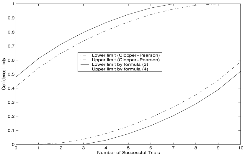
Figure 1. Confidence Interval ($N=10,\;\delta=0.05$.)

Figure 2. Confidence Interval ($N=10,\;\delta=0.01$.)

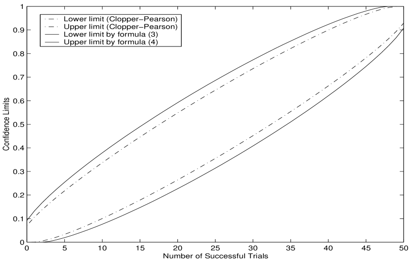
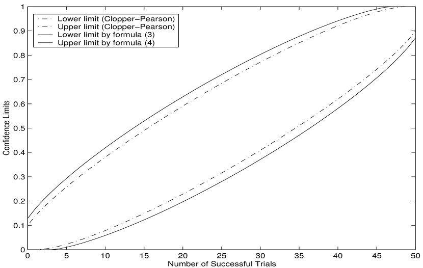
Figure 3. Confidence Interval ($N=50,\;\delta=0.05$.)

Figure 4. Confidence Interval ($N=50,\;\delta=0.01$.)

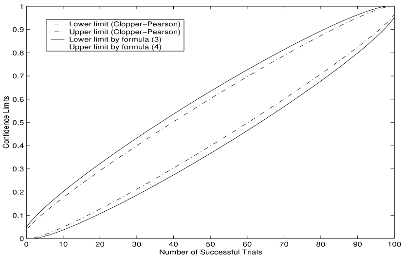
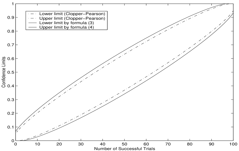
Figure 5. Confidence Interval ($N=100,\;\delta=0.05$.)

Figure 6. Confidence Interval ($N=100,\;\delta=0.01$.)

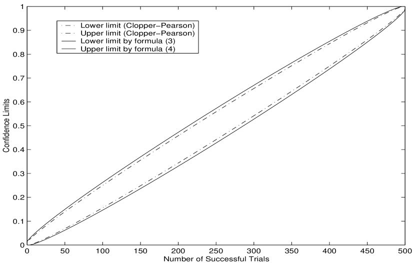
Figure 7. Confidence Interval ($N=500,\;\delta=0.05$.)

Figure 8. Confidence Interval ($N=500,\;\delta=0.01$.)

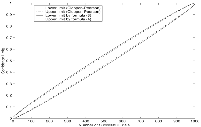
Figure 9. Confidence Interval ($N=1000,\;\delta=0.05$.)

Figure 10. Confidence Interval ($N=1000,\;\delta=0.01$.)

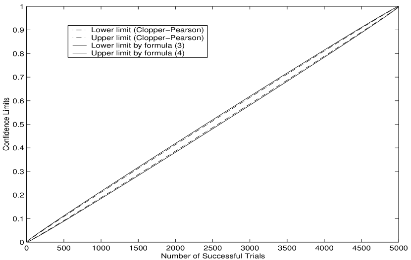
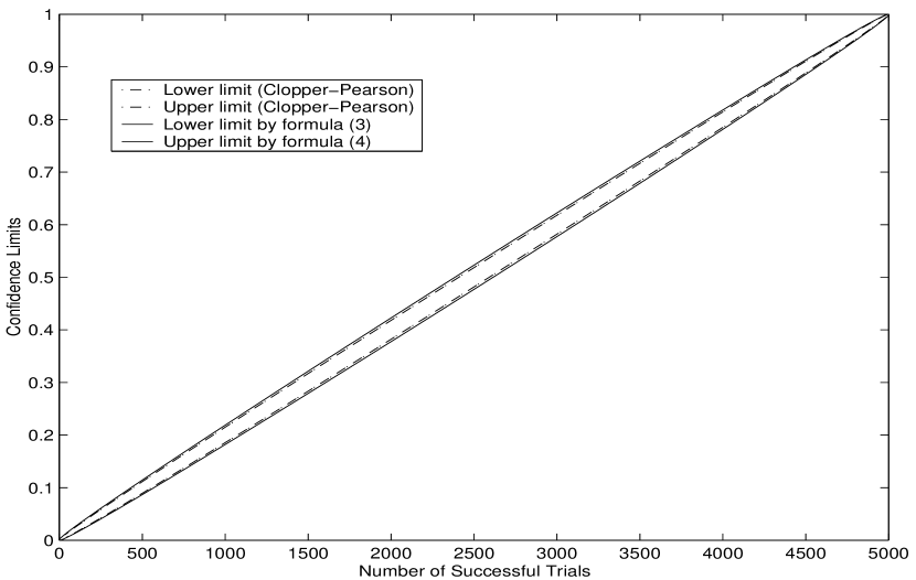
Figure 11. Confidence Interval ($N=5000,\;\delta=0.05$.)

Figure 12. Confidence Interval ($N=5000,\;\delta=0.01$.)

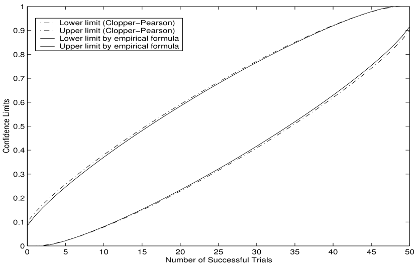
Figure 13. Confidence Interval ($N=50,\;\delta=0.05$.)

Figure 14. Confidence Interval ($N=50,\;\delta=0.01$.)

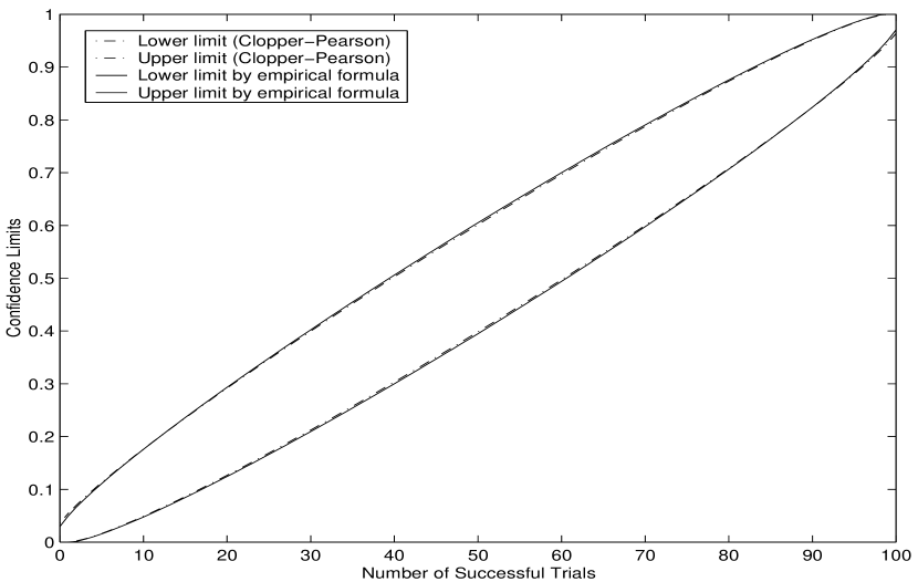
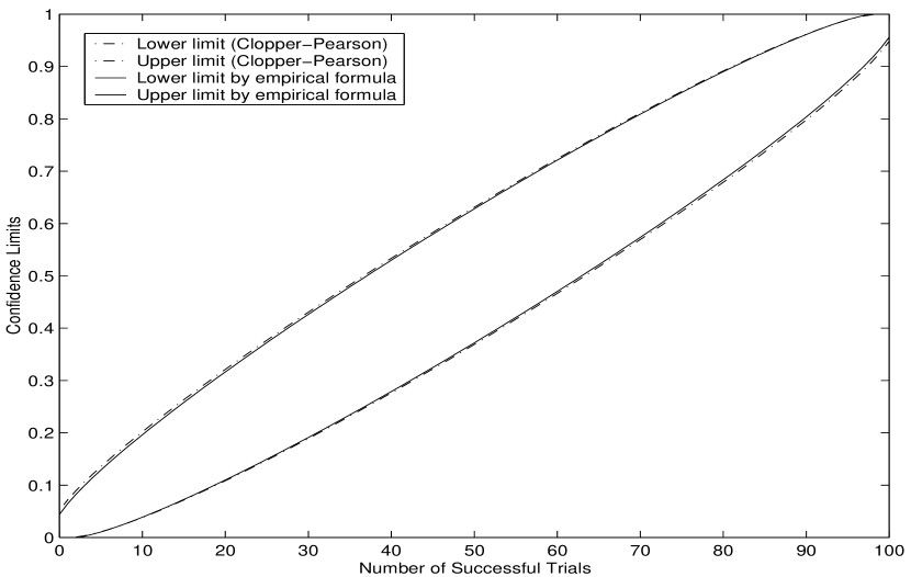
Figure 15. Confidence Interval ($N=100,\;\delta=0.05$.)

Figure 16. Confidence Interval ($N=100,\;\delta=0.01$.)

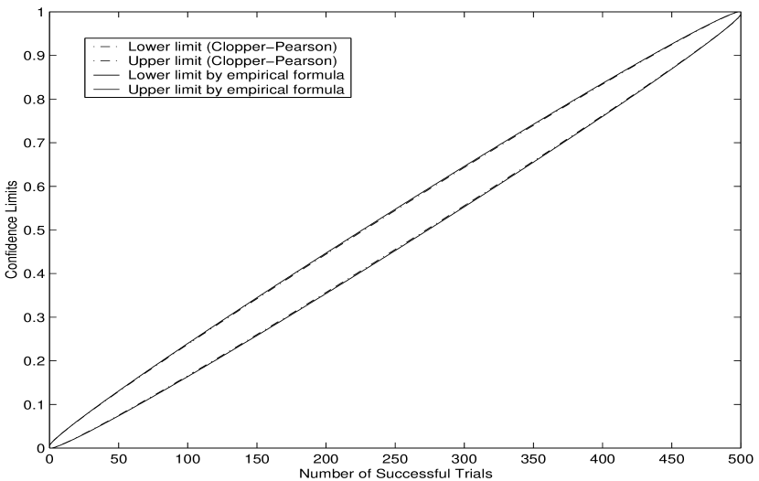
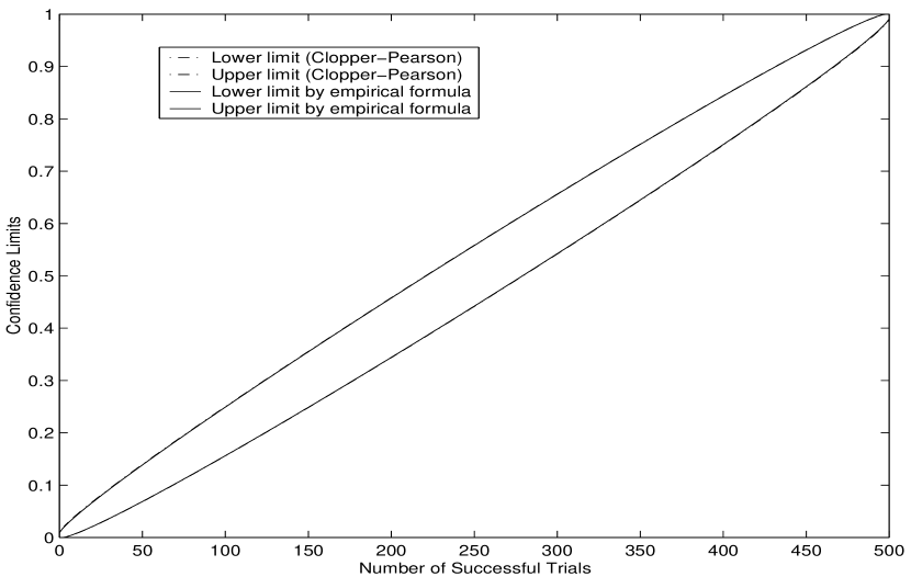
Figure 17. Confidence Interval ($N=500,\;\delta=0.05$.)

Figure 18. Confidence Interval ($N=500,\;\delta=0.01$.)

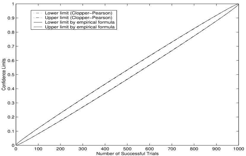
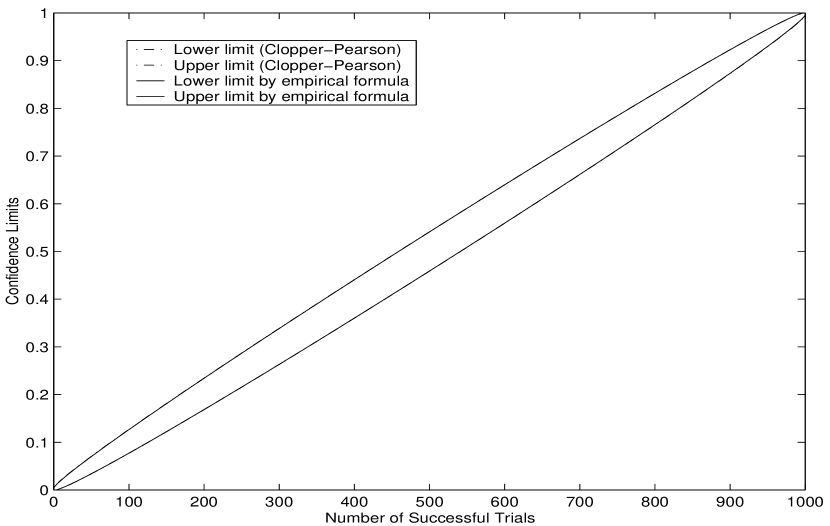
Figure 19. Confidence Interval ($N=1000,\;\delta=0.05$.)

Figure 20. Confidence Interval ($N=1000,\;\delta=0.01$.)

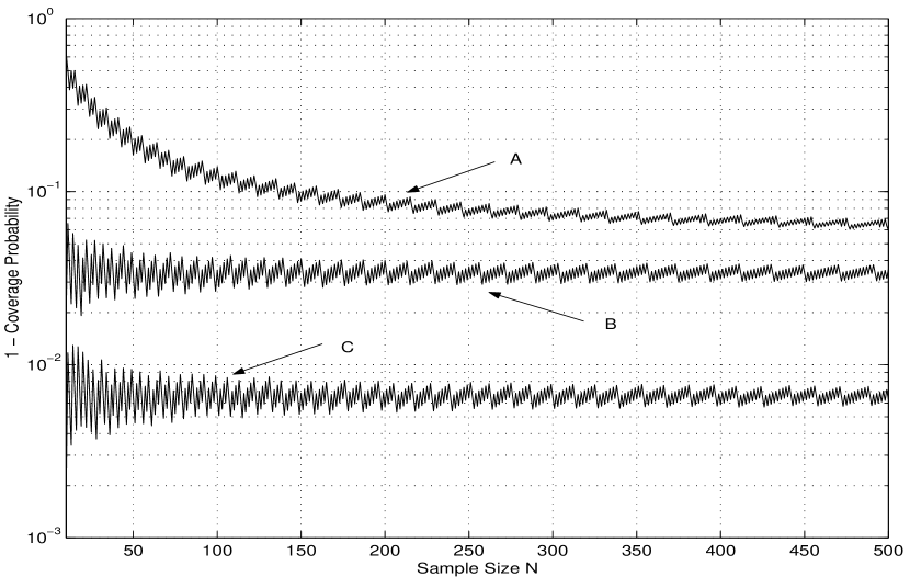
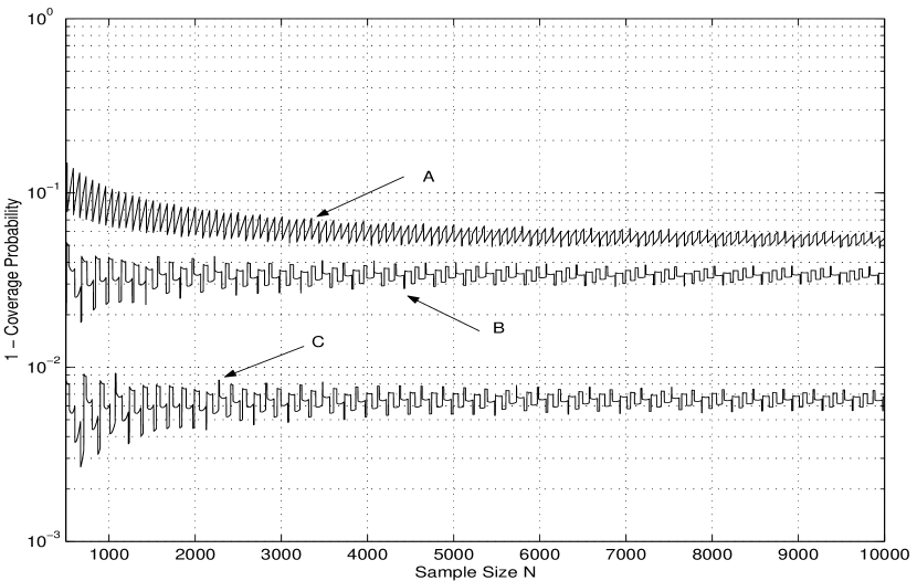
Figure 21. Error Probability ($\mathbb{P}_{X}=0.5,\;\delta=0.05$. A – Normal, B – Empirical, C – Rigorous )

Figure 22. Error Probability ($\mathbb{P}_{X}=0.01,\;\delta=0.05$. A – Normal, B – Empirical, C – Rigorous)

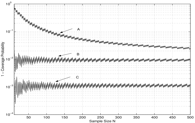
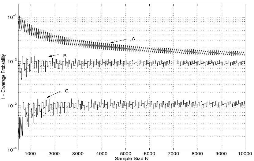
Figure 23. Error Probability ($\mathbb{P}_{X}=0.5,\;\delta=10^{-2}$. A – Normal, B – Empirical, C – Rigorous)

Figure 24. Error Probability ($\mathbb{P}_{X}=0.01,\;\delta=10^{-2}$. A – Normal, B – Empirical, C – Rigorous)

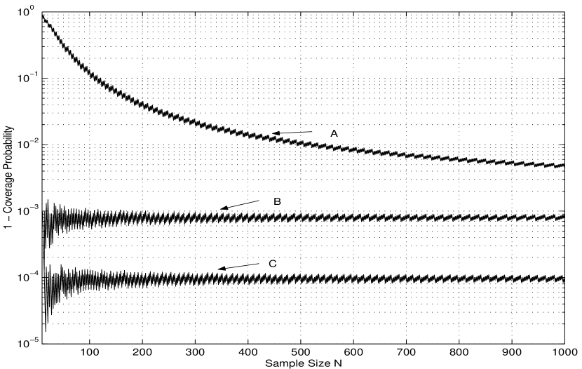
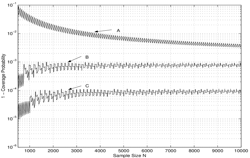
Figure 25. Error Probability ($\mathbb{P}_{X}=0.5,\;\delta=10^{-3}$. A – Normal, B – Empirical, C – Rigorous)

Figure 26. Error Probability ($\mathbb{P}_{X}=10^{-2},\;\delta=10^{-3}$. A – Normal, B – Empirical, C – Rigorous)

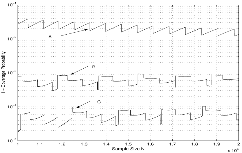
Figure 27. Error Probability ($\mathbb{P}_{X}=10^{-5},\;\delta=10^{-3}$. A – Normal, B – Empirical, C – Rigorous)

References

- [1] Brown, L. D. Cai, T. DasGupta, A. (2001). Interval estimation for a binomial proportion. Statistical Science 16:101-133.
- [2] Brown, L. D. Cai, T. DasGupta, A. (2002). Interval estimation for a binomial proportion and asymptotic expansions. The Annals of Statistics 30:160-201.
- [3] Clopper C. J. Pearson E. S. (1934). The use of confidence or fiducial limits illustrated in the case of the binomial. Biometrika 26:404-413.
- [4] Clunies-Ross, C. W. (1958). Interval estimation for the parameter of a binomial distribution. Biometrika 45:275-279.
- [5] Hald, A. (1952). Statistical Theory with Engineering Applications, pp. 697-700, John Wiley and Sons.
- [6] John, N. Kotz, L. S. Kemp, A. W. (1992) Univariate Discrete Distributions, 2rd ed., pp. 124-130, Wiley.
- [7] Massart, P. (1990). The tight constant in the Dvoretzky-Kiefer-Wolfowitz inequality. The Annals of Probability 18:1269-1283.