Signatures of Extra Gauge Bosons in the Littlest Higgs Model with T-parity at Future Colliders

Abstract

We study the collider signatures of a T-odd gauge boson $W_{H}$ pair production in the Littlest Higgs Model with T-parity (LHT) at Large Hadron Collider (LHC) and Linear Collider (LC). At the LHC, we search for the $W_{H}$ boson using its leptonic decay, i.e. $pp\to W_{H}^{+}W_{H}^{-}\to A_{H}A_{H}\ell^{+}\nu_{\ell}\ell^{\prime-}\bar{\nu}_{\ell^{\prime}}$, which gives rise to a collider signature of $\ell^{+}\ell^{\prime-}+\not\!\!E_{T}$. We demonstrate that the LHC not only has a great potential of discovering the $W_{H}$ boson in this channel, but also can probe enormous parameter space of the LHT. Due to four missing particles in the final state, one cannot reconstruct the mass of $W_{H}$ at the LHC. But such a mass measurement can be easily achieved at the LC in the process of $e^{+}e^{-}\to W_{H}^{+}W_{H}^{-}\to A_{H}A_{H}W^{+}W^{-}\to A_{H}A_{H}jjjj$. We present an algorithm of measuring the mass and spin of the $W_{H}$ boson at the LC. Furthermore, we illustrate that the spin correlation between the $W$ boson and its mother particle ($W_{H}$) can be used to distinguish the LHT from other new physics models.

I introduction

It has been shown that the collective symmetry breaking mechanism implemented in Little Higgs models Arkani-Hamed et al. (2001) provides an interesting solution to the “little hierarchy problem” (also see Schmaltz and Tucker-Smith (2005); Perelstein (2007) for recent review). The Littlest Higgs model, a $SU(5)/SO(5)$ nonlinear sigma model proposed in Ref. Arkani-Hamed et al. (2002), is one of the most economical and interesting models discussed in the literature. In the Littlest Higgs Model, the global symmetry $SU(5)$ is broken down to $SO(5)$ by a $5\times 5$ symmetric tensor at the scale $f$. Simultaneously, the gauged $[SU(2)\times U(1)]_{1}\times[SU(2)\times U(1)]_{2}$, a subgroup of $SU(5)$, is broken to the diagonal $SU(2)_{W}\times U(1)_{Y}$, a subgroup of $SO(5)$. A vector-like quark, $T_{+}$, is introduced in the top sector to cancel the quadratic divergence contribution to Higgs boson mass from the Standard Model (SM) top quark loop. The low energy electroweak precision tests (EWPT), however, enforce the symmetry breaking scale $f$ to be larger than about $4\,{\rm TeV}$. As a result, the cut-off scale $\Lambda\sim 4\pi f$ becomes so large that the fine tuning between the cut-off scale and the electroweak scale is needed again Csaki et al. (2003a, b); Hewett et al. (2003); Chen and Dawson (2004); Kilian and Reuter (2004); Han and Skiba (2005). The Littlest Higgs model with T-parity (LHT) Cheng and Low (2003, 2004); Low (2004) was proposed by imposing a discrete $Z_{2}$ symmetry, called T-parity, into the Littlest Higgs model. T-parity Cheng and Low (2003, 2004); Low (2004) is a symmetry which exchanges the gauge boson fields of the two gauged $SU(2)\times U(1)$ groups, i.e. $[SU(2)\times U(1)]_{1}\leftrightarrow[SU(2)\times U(1)]_{2}$. One direct consequence of the T-parity is the absence of the mixing between the extra heavy gauge bosons and the SM gauge bosons, because they have different T-parity quantum numbers. The constraints from EWPT are alleviated so that the scale $f$ could be as low as $500\,{\rm GeV}$ Hubisz et al. (2006).

In order to incorporate the T-parity systematically, extra fermion fields have to be introduced. One needs two sets of gauge boson fields and fermion fields transforming independently under $[SU(2)\times U(1)]_{1,\,2}$. One of the two possible linear combinations of the fields from two different sets is assigned to be the SM field and another combination is the extra heavy field. The heavy particles (except the vector-like $T_{+}$) are odd under the T-parity while the SM particles are even. With the exact T-parity embedded, the effective operators which mix T-odd and T-even fields are absent. Details of the LHT considered in this paper have been shown in Refs. Hubisz and Meade (2005); Belyaev et al. (2006). Here, we only layout the mass spectrum of the particles relevant to our study, which are $A_{H}$ (T-parity partner of photon), $W_{H}$ (T-parity partner of $W$ boson), $\ell_{-}$ (T-odd lepton) and $q_{-}$ (T-odd quark) ,

$$m_{A_{H}} \simeq \frac{g^{\prime}f}{\sqrt{5}},\,\,m_{W_{H}}\simeq gf,\,\,m_{\ell_{-}}\simeq\sqrt{2}\kappa_{\ell}f\,,\,\,m_{q_{-}}\simeq\sqrt{2}\kappa_{q}f,$$

where $g^{\prime}$ and $g$ are the hypercharge and weak gauge coupling, respectively, and $\kappa_{\ell}$ ($\kappa_{q}$) is the Yukawa type coupling introduced in the interaction which generates the T-odd lepton (quark) mass. $A_{H}$ is usually the lightest T-odd particle (LTP) which cannot further decay into the SM particles and thus plays as the dark matter candidate. With the allowed low mass scale, these extra T-odd particles have significant impacts on the phenomenology Chen et al. (2006); Choudhury et al. (2006a); Blanke et al. (2006a); Hundi et al. (2006); Cao et al. (2006); Blanke et al. (2006b, 2007a, 2007b, 2007c, 2007d); Choudhury et al. (2006b); Yue and Zhang (2007); Chen et al. (2007); Hong-Sheng (2007); Kai et al. (2007); Wang et al. (2007); Yue et al. (2007). Large Hadron Collider (LHC) at CERN has a great potential to copiously produce these new particles. Some studies about collider phenomenology of the LHT have been presented recently Hubisz and Meade (2005); Freitas and Wyler (2006); Belyaev et al. (2006); Matsumoto et al. (2006); Choudhury and Ghosh (2006); Carena et al. (2007); Cao et al. (2006).

Current EWPT only impose constraints on the parameter space of the LHT. Due to the T-parity, the new T-odd particles have to be produced in pairs at the colliders. The fact that at least two missing particles remain in the final state makes it difficult to measure the model parameters of the LHT, see details in the discussions of the LHC phenomenology. In order to test the LHT at the LHC, one has to observe the new physics signatures in various independent channels. By comparing the model parameters extracted out from those channels one might be able to check the consistency of the LHT. For that, the $W_{H}^{+}W_{H}^{-}$ production is of importance because the mass of the heavy gauge boson $W_{H}$ ($m_{W_{H}}$) depends on $f$ only. One thus can directly determine the symmetry breaking scale $f$ from the $W_{H}$ mass measurement . In this paper, we examine the discovery potential of the $W_{H}^{+}W_{H}^{-}$ pair production at the LHC and present a strategy of measuring the mass and spin of $W_{H}$ at the LC. The matrix elements of both signal and background processes are calculated using MadGraph Stelzer and Long (1994); Maltoni and Stelzer (2003) while the widths of the new T-odd particles are calculated in CalcHEP Pukhov (2004) with the model file given by Ref. Belyaev et al. (2006). Agreement of both programs at the level of new gauge boson production has been checked. The rest of this paper is organized as follows. In Sec. II, we present the cross sections of the $W_{H}^{+}W_{H}^{-}$ pair production at the LHC and at the LC. We also discuss the decay pattern of $W_{H}$ and present the unitarity constraints on the parameter space of the LHT from effective four fermion interaction operators. The collider phenomenology of the LHC and the LC is shown in Sec. III and Sec. IV, respectively. Finally, we conclude in Sec. V.

II production and decay of $W_{H}$ boson 

The tree-level diagrams for a $W_{H}$ pair production are shown in Fig. 1, where $F$ and $F^{\prime}$ denote the quarks at the LHC while the electron and electron-neutrino at the LC. The $W_{H}$ boson pair can be produced either via the $s$-channel process with the photon and $Z$ boson exchanged or via the $t$-channel process with a T-odd fermion exchanged. Since the $t$-channel diagram involves the heavy T-odd fermion, its contribution depends on both $m_{W_{H}}$ and $m_{F_{-}}$. In this work we choose the model parameters ($f$, $\kappa_{q/\ell}$) instead of the physical masses of the new particles as the theoretical inputs.

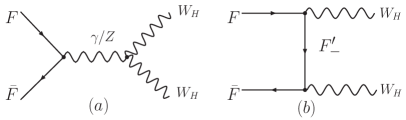
Figure 1: Feynman diagrams for a $W_{H}$ pair production.

II.1 $W_{H}$ production at the LHC

In Fig. 2(a) and 2(b) we show the total cross section of the $W_{H}$ pair production as a function of $\kappa_{q}$ and $f$, respectively. The T-odd quark in the $t$-channel diagram affects the total cross section significantly: (i) for $500\,{\rm GeV}<f<1000\,{\rm GeV}$, there exists a $\kappa_{q}^{min}$($\sim 0.6$) which minimizes the total cross section; (ii) for a fixed $\kappa_{q}$, the cross section decreases rapidly with increasing $f$. In order to understand why the minimum of the total cross section occurs, we separate the total cross section into three pieces,

$$\sigma_{tot}=\sigma_{s}+\sigma_{t}+\sigma_{{\rm int}},$$ (1)

where $\sigma_{s}$, $\sigma_{t}$ and $\sigma_{{\rm int}}$ denote the contributions of the $s$-channel diagram, $t$-channel diagram and the interference between the $s$- and $t$-channel diagrams, respectively. For illustration, we choose $f=500\,{\rm GeV}$ and plot each individual contribution in Fig. 2(c). The $s$-channel diagram involves the gauge bosons only, therefore, its contribution depends on $f$ but not on $\kappa_{q}$, cf. the flat blue curve. On the contrary, the $t$-channel contribution decreases with increasing $\kappa_{q}$, because the mass of the T-odd quark in the $t$-channel propagator grows with increasing $\kappa_{q}$, cf. the red curve. Although the $s$-channel and $t$-channel contributions are both constructive, their interference is destructive. The total cross section reaches the minimum when $\kappa_{q}\sim\kappa_{q}^{min}$, where the $s$- and $t$-channel contributions are comparable. When $\kappa_{q}>\kappa_{q}^{min}$, the total cross section is dominated by the $s$-channel contribution, therefore it drops rapidly with increasing $f$ since the $s$-channel contribution suffers from the $1/\hat{s}$ suppression ( $\hat{s}$ is the invariant mass of the $W_{H}$ boson pair). When $\kappa_{q}\gg\kappa_{q}^{min}$, the total cross section approaches to the $s$-channel contribution and both the $t$-channel contribution and the interference effect are negligible.

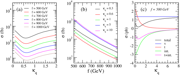
Figure 2: The total cross section of a $W_{H}^{+}W_{H}^{-}$ pair production at the LHC for various parameters $f$ and $\kappa_{q}$. 

II.2 $W_{H}$ production at the LC

We present the total cross section of the $W_{H}$ pair production at the LC as a function of $\kappa_{\ell}$ and $f$ in Fig. 3(a) and (b), respectively. In analogue to the $W_{H}$ pair production at the LHC, there also exists a $\kappa_{\ell}^{min}$ due to the destructive interference effect, but $\kappa_{\ell}^{min}$ is very sensitive to $f$ at the LC. As shown in Fig. 3(a), $\kappa_{\ell}^{min}$ shifts from about 0.5 to 1.0 when $f$ increases from 500 GeV to 750 GeV. We also note that the total cross section of a small $\kappa_{\ell}$, e.g. $\kappa_{\ell}=0.3$, drops much slower than the total cross section of a large $\kappa_{\ell}$, see Fig. 3(b).

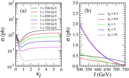
Figure 3: Total cross section of a $W_{H}^{+}W_{H}^{-}$ pair production at the LC for various $f$ and $\kappa_{\ell}$. 

Following the LHC study, we split the total cross section into the $s$-channel, $t$-channel and the interference contributions. In Fig. 4 we explicitly plot the total cross section (black curve), the $s$-channel contribution (blue curve), the $t$-channel contribution (red curve) and the interference contribution (INT) (green curve). Fig. 4(a) and (b) show the total cross section as a function of $\kappa_{\ell}$ for $f=500\,{\rm GeV}$ and $750\,{\rm GeV}$, respectively. We have learned from the LHC study that the minimal cross section for a fixed $f$ occurs when $\sigma(s)\simeq\sigma(t)$. When $f$ increases from 500 GeV to 750 GeV, the $s$-channel contribution drops rapidly since it suffers from the $1/\hat{s}$ suppression, but on the other hand, the $t$-channel contribution does not. Of course, increasing $f$ value will increase the mass of $W_{H}$ boson and reduce the $t$-channel contribution, but the suppression in the $t$-channel contribution is much less than that in the $s$-channel contribution. Therefore, the position for $\sigma(s)\simeq\sigma(t)$ is shifted to larger $\kappa_{\ell}$ region. The reason why the cross section of $\kappa_{\ell}=0.3$ drops slowly in the large $f$ region can also be understood from the competition between the $s$- and $t$-channel contributions. In Fig. 4(c) we show the total cross section as a function of $f$ for $\kappa_{\ell}=0.3.$ For such a small $\kappa_{\ell}$, the T-odd neutrino’s mass is small ($m_{\nu-}\simeq 0.42f$). Then the $t$-channel contribution dominates over the $s$-channel contribution. In the large $f$ region, i.e. $600\,{\rm GeV}<f<750\,{\rm GeV}$, the $s$-channel contribution as well as the interference effect both decrease to zero, and the total cross section approaches to the $t$-channel contribution which does not drop rapidly with increasing $f$.

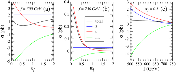
Figure 4: The distributions of $s-$, $t-$channel diagrams and interference term in the $W_{H}^{+}W_{H}^{-}$ production at the LC. 

II.3 Decay of the $W_{H}$ boson

The $W_{H}$ boson will decay into a T-odd particle and a T-even SM particle. Its decay pattern is mainly determined by the masses of new T-odd particles. In the LHT,

$$m_{A_{H}}\simeq\frac{g^{\prime}f}{\sqrt{5}}\simeq 0.156f, m_{W_{H}}\simeq gf\simeq 0.653f,$$

$$m_{\ell-}\simeq\sqrt{2}\kappa_{\ell}f\simeq 1.414\kappa_{\ell}f, m_{q-}\simeq\sqrt{2}\kappa_{q}f\simeq 1.414\kappa_{q}\,f.$$ (2)

It is clear that the $A_{H}$ boson is always lighter than the $W_{H}$ boson. But the T-odd quark (lepton) can be heavier or lighter than the $W_{H}$ boson, depending on the parameter $\kappa_{q}$($\kappa_{\ell}$). Let us denote $F_{-}$ as the T-odd fermion whose mass $m_{F_{-}}$ is $\sqrt{2}\kappa f$. When $\kappa<0.11$, $m_{F_{-}}<m_{A_{H}}<m_{W_{H}}$, therefore the T-odd lepton or T-odd quark will play the role as the dark matter candidate. As pointed out in Ref. Primack et al. (1988), the dark matter candidates should be charge neutral and colorless objects. Hence, we focus our attention to the case of $\kappa_{\ell}\,(\kappa_{q})>0.11$ throughout this study, i.e. demanding $A_{H}$ to be the lightest T-odd particle. When both $\kappa_{q}$ and $\kappa_{\ell}$ are larger than 0.462, i.e. $m_{A_{H}}<m_{W_{H}}<m_{F_{-}}$, the $W_{H}$ boson only decays via the $W_{H}\to W+A_{H}$ channel. When $0.11<\kappa<0.462$, i.e. $m_{A_{H}}<m_{F_{-}}<m_{W_{H}}$, then $W_{H}$ boson can decay into either $WA_{H}$ or $F_{-}F^{\prime}$ ($F^{\prime}$ being the usual SM fermion).

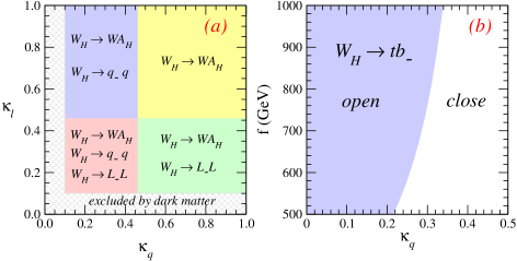
Figure 5: (a) Pictorial illustration of the decay pattern of the $W_{H}$ boson in the plane of $\kappa_{\ell}$ and $\kappa_{q}$ ; (b) allowed region (blue) of $\kappa_{q}$ for the $W_{H}\to tb_{-}$ mode being opened.

In Fig. 5(a) we summarize the decay pattern of $W_{H}$ in the plane of $\kappa_{q}$ and $\kappa_{\ell}$, where the following decay modes are considered:

$$W_{H} \to WA_{H}\to\ell\bar{\ell}^{\prime}\left(q\bar{q}^{\prime}\right)A_{H},$$ (3)

$$W_{H} \to \ell_{-}\nu_{\ell}\to\ell A_{H}\nu_{\ell},$$ (4)

$$W_{H} \to \nu_{\ell-}\ell\to\nu_{\ell}A_{H}\ell,$$ (5)

$$W_{H} \to q_{-}q^{\prime}\to qA_{H}q^{\prime}.$$ (6)

Here, $\ell$($\nu$,$q$) denotes the charged leptons (neutrinos, quarks). We also include the subsequent decay of the second T-odd fermions whose decay branching ratio is 100% for $0.11<\kappa<0.462$. In the above decay modes, the $W_{H}\to tb_{-}\to tbA_{H}$ mode is special because of large top quark mass ($m_{t}$). In order to open the decay mode $W_{H}\to tb_{-}$, the mass constraint $m_{W_{H}}>m_{t}+m_{b_{-}}$ has to be satisfied and the allowed region of $\kappa_{q}$ and $f$ is shown in Fig. 5(b). As shown in Eq. (2), the mass relation between the $W_{H}$, $A_{H}$ and $F_{-}$ is fixed by $\kappa$ and does not depend on $f$. Thus, the decay branching ratios of the $W_{H}\to WA_{H}$ and $W_{H}\to F_{-}F^{\prime}$ modes do not depend on $f$ if the $tb_{-}$ mode is not opened. Once the $tb_{-}$ mode is opened, the decay branching ratios of other modes will be slightly reduced. In Fig. 6 we show the decay branching ratios of the $W_{H}$ boson as a function of $\kappa_{\ell}$ and $\kappa_{q}$, respectively. Explicit numbers of the decay branching ratios for the selected benchmark points are listed in table 1.

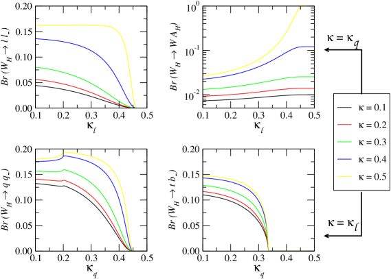
Figure 6: Decay branching ratios of the $W_{H}$ boson for $f=500\,{\rm GeV}$.

Table 1: Decay branching ratios ($\%$) of the $W_{H}$ boson for a few benchmark points, where $\ell=e,\mu,\tau$, $\nu=\nu_{e},\nu_{\mu},\nu_{\tau}$, $U=u,c$ and $D=d,s$. Note that all the SM fermions (except the top quark) are treated as massless.  

	$\kappa_{\ell}=0.3$  $\kappa_{q}=0.3$			$\kappa_{\ell}=0.5$   $\kappa_{q}=0.3$			$\kappa_{\ell}=0.3$  $\kappa_{q}=0.5$			$\kappa_{\ell}=0.5$  $\kappa_{q}=0.5$
$f$(GeV)	500	700	1000	500	700	1000	500	700	1000	$>500$
$\ell_{-}\nu$	4.45	4.61	4.33	0	0	0	15.0	15.9	16.3	0
$\nu_{-}\ell$	4.84	4.81	4.41	0	0	0	16.3	16.5	16.6	0
$U_{-}D$	14.5	14.4	13.2	20.1	20.1	17.9	0	0	0	0
$D_{-}U$	13.4	13.8	13.0	18.5	19.3	17.6	0	0	0	0
$t_{-}b$	14.5	14.4	13.2	20.1	20.1	17.9	0	0	0	0
$tb_{-}$	0	0	7.79	0	0	10.6	0	0	0	0
$WA_{H}$	1.84	0.8	0.33	2.55	1.12	0.45	6.19	2.76	1.25	100

II.4 Unitarity constraints on $\kappa_{q}$ and $\kappa_{\ell}$

Let us examine the low energy constraints on $\kappa_{\ell}$ and $\kappa_{q}$ in this section before studying the phenomenology of the $W_{H}$ boson. The mass constraints on T-odd fermion, i.e. the lepton ($\ell_{-}$) and quark ($q_{-}$), could be derived from four-fermion interaction operators $O(ffff)$.

The most general chirally invariant form of the four fermion interaction reads

$$\frac{g^{2}}{2\Lambda^{2}}\bar{\psi}_{L}\gamma^{\mu}\psi_{L}\bar{\psi}_{L}\gamma_{\mu}\psi_{L},$$

where $\Lambda$ is the new physics scale. One then can determine the scale $\Lambda$ unambiguously from the unitarity condition by setting $g^{2}(\Lambda)/4\pi=1$ for the new strong interaction coupling. For example, $\Lambda(eeee)\,>10.3\,{\rm TeV}$, $\Lambda(eedd)\,>26.4\,{\rm TeV},$ and $\Lambda(uudd)\,>2.4\,{\rm TeV}$ at $95\%$ confidence level Yao et al. (2006). Using these limits, we can calculate the upper bound on T-odd fermion masses. If we assume the universal mass for T-odd lepton ($\ell_{-}$) and quark ($q_{-}$), i.e. $\kappa_{\ell}=\kappa_{q}=\kappa$, the strongest constraint is from $O(eedd)$ Hubisz et al. (2006), which leads to

$$\kappa_{\ell}=\kappa_{q}\leq 3.4\frac{f}{{\rm TeV}}\,.$$ (7)

However, there is no physics reason to believe that the lepton and quark sectors will share the same $\kappa$. In this work we will treat $\kappa_{\ell}$ and $\kappa_{q}$ separately. As a result, the masses of the T-odd leptons differ from the masses of the T-odd quarks. In order to avoid the problem of flavor changing neutral current (FCNC), we further assume $\kappa_{\ell}$ and $\kappa_{q}$ are universal individually and also diagonal in the flavor space. Under this assumption, we obtain the constraints on $\kappa_{\ell}$ and $\kappa_{q}$ separately from $O(eeee)$ and $O(uudd)$ as follows:

$$\kappa_{\ell} \leq 8.6\frac{f}{{\rm TeV}},$$ (8)

$$\kappa_{q} \leq 37.1\frac{f}{{\rm TeV}}.$$ (9)

However, $\kappa_{q}$ and $\kappa_{\ell}$ are correlated by the $O(eedd)$ which leads to

$$\frac{\kappa_{\ell}^{2}\kappa_{q}^{2}}{\kappa_{\ell}^{2}-\kappa_{q}^{2}}{\rm ln}(\frac{\kappa_{\ell}}{\kappa_{q}})\,\leq\frac{128\pi^{3}f^{2}}{(26.4\,{\rm TeV})^{2}}\,.$$ (10)

Fig. 7 shows the correlation of Eq. (10) for various values of $f$. The region below each curve is the allowed parameter space of $\kappa_{\ell}$ and $\kappa_{q}$ for the corresponding $f$. The constraint is tight for small $f$: when $f=500\,{\rm GeV}$, large $\kappa_{q}$ prefers smaller $\kappa_{\ell}$ and vice versa, for example, $\kappa_{q}>4$ requires $\kappa_{\ell}<1$. This constraint becomes quite loose when $f$ becomes large.

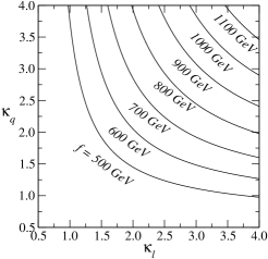
Figure 7: Allowed region of $\kappa_{\ell}$ and $\kappa_{q}$ for various values of $f$. The region below each curve is allowed.

III Phenomenology of the $W_{H}$ pair production at the LHC

The production rate of $W_{H}^{+}W_{H}^{-}$ pair at the LHC is sizable, but the detection for its signatures at the hadron collider was expected to be challenging Hubisz and Meade (2005); Belyaev et al. (2006). However, in this work we will demonstrate that the LHC not only has a great potential to discover the collider signature of the $W_{H}^{+}W_{H}^{-}$ pair production, but also has the capability to explore enormous parameter space of $f$ and $\kappa$. Below we present a detailed study of the LHC phenomenology.

At the LHC, we demand the two $W_{H}$ bosons both decay leptonically in order to avoid the huge QCD backgrounds. We further require the two charged leptons in the final state having different lepton flavors. Hence, the collider signature of the signal events is $e^{+}\mu^{-}\not\!\!E_{T}$ (or $e^{-}\mu^{+}\not\!\!E_{T}$), where the missing energy ($\not\!\!E_{T}$) is originated from two $A_{H}$’s and two neutrinos. For simplicity, we will present the study of $e^{+}\mu^{-}\not\!\!E_{T}$ signature throughout this paper, but it is very straightforward to include the contribution of $e^{-}\mu^{+}\not\!\!E_{T}$ mode as those two decay modes are identical .

When $W_{H}$ is the second lightest T-odd particle, i.e. $\kappa_{q}$ and $\kappa_{\ell}$ are both larger than 0.462, the signal events only come from the following process

$$pp\to W_{H}^{+}W_{H}^{-}\to A_{H}W^{+}(\to e^{+}\nu_{e})A_{H}W^{-}(\to\mu^{-}\bar{\nu}_{\mu}).$$ (11)

However, when the T-odd leptons are lighter than $W_{H}$, i.e. $\kappa_{\ell}<0.462$, the signal will mainly come from the process

$$pp\to W_{H}^{+}W_{H}^{-}\to\ell_{1-}\ell_{2}\ell_{3-}\ell_{4}\to e^{+}\mu^{-}\nu_{e}\bar{\nu}_{\mu}A_{H}A_{H},$$ (12)

where $\ell_{i}=e,\,\mu,\,\nu_{e}$ or $\nu_{\mu}$. The total cross sections of these two processes are shown in Fig. 8 where the left plot is for the process in Eq. (11) with $\kappa_{\ell}=0.5$ while the right plot is for the process in Eq. (12) with $\kappa_{\ell}=0.3$. If $W_{H}$ is the second lightest T-odd particle, the signal will only come from Eq. (11) since the $W_{H}$ can only decay to $WA_{H}$; otherwise, the process in Eq. (12) dominates. The total rate of the signal events depends on the masses of $\ell_{-}$, $q_{-}$ and $W_{H}$, and as shown in Fig. 8, the total cross section is sizable when $f$ is small and $\kappa_{q}$ is large. This is because that the mass of T-odd gauge boson is light and the destructive effect from t-channel and s-channel interference term is small.

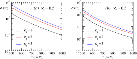
Figure 8: The total cross section of $pp\to W_{H}^{+}W_{H}^{-}\to e^{+}\mu^{-}\not\!\!E_{T}$ at the LHC. 

The main intrinsic backgrounds come from the $W^{+}W^{-}$ and the $ZW^{+}W^{-}$ continuum productions with the subsequent decays $W^{+}\to\ell^{+}\nu_{\ell}$, $W^{-}\to\ell^{-}\bar{\nu}_{\ell}$ and $Z\to\nu\nu$ . There also exist other reducible backgrounds from the top quark pair production and the $Wt$ associated production which can be highly suppressed by vetoing the additional $b$-jet from the top quark decay with large transverse momentum or in the central rapidity region. The vetoing efficiency is so large, about $99.9\%$ for the $t\bar{t}$ background and $99.6\%$ for the $Wt$ background, that we only need to consider the intrinsic backgrounds in this study. The total cross section of the $W^{+}W^{-}$ pair production background is about $0.865\,{\rm pb}$ while the other intrinsic background from $W^{+}W^{-}Z$ is negligible ($\sim 0.08\,{\rm fb}$). These cross sections already include the decay branching ratios of $W\to\ell\nu$ and $Z\to\nu\nu$. Below, we just consider the $W^{+}W^{-}$ pair production as the background at the LHC.

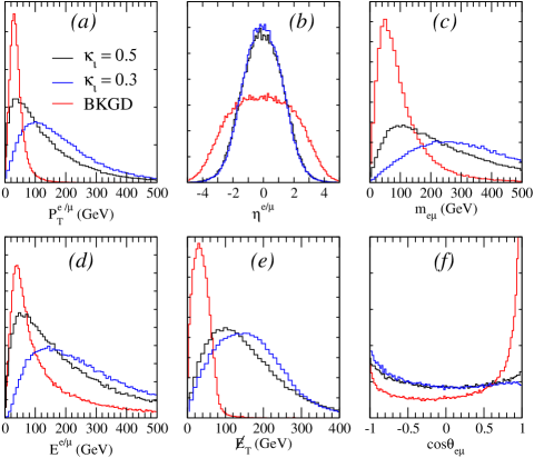
Figure 9: Transverse momentum of $e^{+}/\mu^{-}$ ($p_{T}^{e/\mu}$), rapidity of $e^{+}/\mu^{-}$ ($\eta^{e/\mu}$), invariant mass of $e^{+}$ and $\mu^{-}$ ($m_{e\mu}$), energy of $e^{+}/\mu^{-}$ ($E^{e/\mu})$, missing transverse momentum ($\not\!\!E_{T}$), cosine of the opening angle between $e^{+}$ and $\mu^{-}$($\cos\theta_{e\mu}$) distributions for $\kappa_{q}=1$ and $f=700\,{\rm GeV}$. All curves are normalized by their total cross sections. 

Kinematics of the signal events is distinctively different from that of background events. As to be shown later, these differences can be used to significantly suppress the background and enhance the ratio of signal to background ($S/B$). For illustration, we show normalized distributions of various kinematics observables of the signal and background events in Fig. 9: transverse momentum $(p_{T}^{e/\mu})$, rapidity $(\eta^{e/\mu})$, energy $(E^{e/\mu})$ of charged leptons, invariant mass of two charged leptons ($m_{e\mu}$), missing transverse momentum ($\not\!\!E_{T}$) and cosine of the opening angle between two charged leptons ($\cos\theta_{e\mu}$). The curves labelled by $\kappa_{\ell}=0.5$ and $\kappa_{\ell}=0.3$ correspond to the signals described in Eq. (11) and Eq. (12), respectively. A few interesting points are summarized below:

• Compared to the background, the typical feature of the signal events is that the final state particles are more energetic, cf. Fig. 9(a), (c), (d), (e).

• As the decay products of heavy $W_{H}$ bosons, the two charged leptons mainly appear in the central region, cf. Fig. 9(b), because $W_{H}$ is hardly boosted.

• We also note that, unlike the background, two charged leptons of the signal do not exhibit strong correlations, see the nearly flat behavior in the $\cos\theta_{e\mu}$ distribution. It can be understand as follows. Since $m_{W_{H}}$ is much larger than $m_{W}$ and $m_{A_{H}}$, $W$ and $A_{H}$ will be predominately in the longitudinal polarization state, i.e. behaving as scalars. Thus, the spin correlation between $e^{+}$ and $\mu^{-}$ is lost, which results in a flat distribution. On the contrary, the two charged leptons in the SM background are highly correlated.

• The signal distributions change a lot when varying the value of $\kappa_{\ell}$. In particular, for a Small $\kappa_{\ell}$, i.e. $\kappa_{\ell}=0.3$, the peak positions of the $p_{T}^{e/\mu}$, $m_{e\mu}$, $E_{e}^{e/\mu}$ and $\not\!\!E_{T}$ distributions are shifted to the large value region when compared to those of large $\kappa_{\ell}$, i.e. $\kappa_{\ell}=0.5$. This is due to the fact that for a small $\kappa_{\ell}$, the charged leptons ($e^{+}$ and $\mu^{-}$) or the neutrinos ($\nu_{e}$ and $\bar{\nu}_{\mu}$) are directly generated from the $W_{H}$ boson decay, e.g. $W_{H}^{+}\to e^{+}\nu_{e_{-}}$ or $W_{H}^{+}\to\nu_{e}e_{-}^{+}$, and therefore are more energetic.

In order to mimic the detector, we require $p_{T}^{e/\mu}$ and $\eta^{e/\mu}$ to satisfy the following basic cuts:

$$p_{T}^{e}>20.0\,{\rm GeV}\,,\,p_{T}^{\mu}>20.0\,{\rm GeV}\,,$$

$$\,|\eta^{e}|<2.0\,\,\,\,\,\,\,\,\,\,\,\,\,,\,|\eta^{\mu}|<2.0\,.$$ (13)

Furthermore, taking advantage of the differences between the kinematics of the signal and background events, we impose the following optimal cuts to extract the signal out of the SM background,

$$\not\!\!E_{T}>175\,{\rm GeV}\,,\,\cos\theta_{e\mu}<0.6\,.$$ (14)

After imposing the optimal cuts, the main background from the $W^{+}W^{-}$ pair production can be suppressed by more than $99\%$ and gives rise to 18 background events for $\mathcal{L}=10\,{\rm fb}^{-1}$ while 192 events for $\mathcal{L}=100\,{\rm fb}^{-1}$, where $\mathcal{L}$ denotes the integrated luminosity. These background rates include both $e^{+}\mu^{-}$ and $e^{-}\mu^{+}$ modes. In Fig. 10 we present the $5\sigma$, $3\sigma$ statistical significance and $95\%$ confidence level (C.L.) for $\kappa_{\ell}=0.5$ (top raw) and $\kappa_{\ell}=0.3$ (bottom raw). For $\kappa_{\ell}=0.5$, the $W_{H}$ boson is the second lightest T-odd particle and the signal events come from Eq. (11) only. When $f$ is $500\,{\rm GeV}$, the signal can reach more than $3\sigma$ statistical significance for $\kappa_{q}\gtrsim 1.5$ with $\mathcal{L}=10\,{\rm fb}^{-1}$ and $\kappa_{q}\gtrsim 1$ with $\mathcal{L}=100\,{\rm fb}^{-1}$, respectively. Furthermore, the $f$ can be probed up to about $770\,{\rm GeV}$ with $\mathcal{L}=10\,{\rm fb}^{-1}$ and $950\,{\rm GeV}$ with $\mathcal{L}=100\,{\rm fb}^{-1}$, respectively, at the $95\%$ C.L.. On the other hand, for $\kappa_{\ell}=0.3$, the T-odd leptons are lighter than $W_{H}$ and the signal events predominantly come from Eq. (12) due to the large decay branching ratios. In this case, one can probe more parameter space of the LHT, cf. Fig. 10(c) and (d). For example, assuming $\kappa_{q}=1$, one can probe $f$ up to $900\,{\rm GeV}$ with $\mathcal{L}=10\,{\rm fb}^{-1}$ and $1050\,{\rm GeV}$ with $\mathcal{L}=100\,{\rm fb}^{-1}$, respectively, at the $5\sigma$ level.

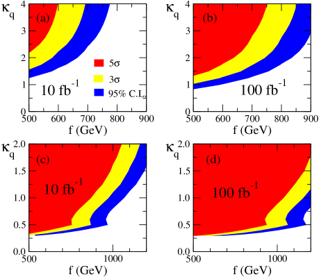
Figure 10: Statistical significance contour of signature of $pp\to W_{H}^{+}W_{H}^{-}\to\ell^{+}\ell^{\prime-}\nu_{\ell}\bar{\nu}_{\ell^{\prime}}A_{H}A_{H}$ in the plane of $\kappa_{q}$ and $f$ at the LHC. The upper two plots are for $\kappa_{\ell}=0.5$ while the lower two are for $\kappa_{\ell}=0.3$. 

As shown above, it is very promising to use the $e\mu+\not\!\!E_{T}$ signature to detect the $W_{H}W_{H}$ pair production at the LHC. But such a signature can originate from two processes, either Eq. (11) or Eq. (12), depending on the value of $\kappa_{\ell}$. Therefore, one immediate task after observing such a signature is to determine from which process it comes. It turns out that this question can be easily answered by the $p_{T}^{e/\mu}$ and $E^{e/\mu}$ distributions, cf. Fig. 11 where we have imposed the optimal cuts. In case of $\kappa_{\ell}=0.3$, the charged lepton is directly emitted from the T-odd gauge boson decay, therefore its transverse momentum is typically larger than the one of the charged lepton emitted form the $W$-boson decay, i.e. $\kappa_{\ell}=0.5$. Same argument also works for the energy distributions. Hence, one can fit the observed $p_{T}^{e/\mu}$ and $E^{e/\mu}$ distributions to the LHT predictions to measure $\kappa_{\ell}$, though $\kappa_{q}$, which merely change the normalization of both distributions, remains unknown.

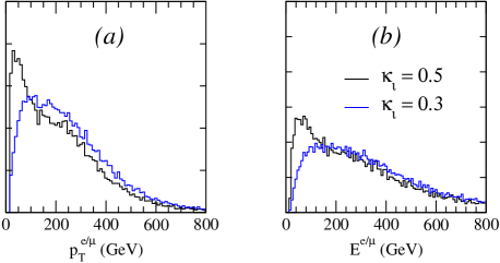
Figure 11: Normalized distributions of $p_{T}^{e/\mu}$ and $E^{e/\mu}$ for $f=700\,{\rm GeV}$ and $\kappa_{q}=1$ for $pp\to W_{H}^{+}W_{H}^{-}\to e^{+}\mu^{-}\nu_{e}\bar{\nu}_{\mu}A_{H}A_{H}$ process after imposing the kinematics cuts given in Eq. (14) at the LHC. 

IV Phenomenology of the $W_{H}$ pair production at the LC 

Compared to the LHC, the LC does not have sufficient energy to produce very heavy $W_{H}$ bosons. For example, the LC can only probe the $W_{H}$ boson mass up to $500\,{\rm GeV}$, which corresponds to $f\simeq 750\,{\rm GeV}$. However, the LC provides a much cleaner experimental environment (no QCD backgrounds) which is perfect for precision measurements. As mentioned before, because of suffering from the extremely huge QCD backgrounds, one has to use the leptonic decay mode for the $W_{H}$ boson search at the LHC. One can observe a deviation from the SM prediction, but one cannot determine the mass or spin of the $W_{H}$ boson due to the four missing particles (two $A_{H}$’s and two neutrinos) in the final state. In this section we preform a comprehensive study of the $W_{H}$ pair production at the LC and address on the following questions:

• Can one determine the masses of $W_{H}$ and $A_{H}$?

• Can we reconstruct the kinematics of the missing particle $A_{H}$?

• Can we measure the spin of $W_{H}$?

As to be shown later, all these questions can be easily answered at the LC with the help of the known center-of-mass (c.m.) energy.

At the LC, we are able to search the $W_{H}$ boson using its hadronic decay mode $W_{H}\to A_{H}W\to A_{H}jj$. Below, we consider the following signal process

$$e^{+}e^{-}\to W_{H}^{+}W_{H}^{-}\to W^{+}(\to jj)W^{-}(\to jj)A_{H}A_{H},$$ (15)

which gives rise to a collider signature of four isolated jets associated with large missing energy originated from the two undetectable $A_{H}$ bosons in the final state. The main intrinsic background is from the process $e^{+}e^{-}\to W^{+}W^{-}Z\to jjjj\nu\bar{\nu}$ whose cross section is about $5.6\,{\rm fb}$. In Fig. 12, we show the cross section of the signal process given in Eq. (15) at the LC. The total cross section relies on how large the decay branching ratio of the $W_{H}\to WA_{H}$ mode is: (1) when both $\kappa_{\ell}$ and $\kappa_{\ell}$ are large, $Br(W_{H}\to WA_{H})=1$ which leads to a large cross section, see the black (solid) curve; (2) when either $\kappa_{q}$ or $\kappa_{\ell}$ is small, $Br(W_{H}\to WA_{H})$ is highly suppressed, so the total cross section becomes small, see the blue (dashed), the red (dotted) and the green (dot-dashed) curves. In this work we focus our attention on the first case, i.e. large $\kappa_{q}$ and $\kappa_{\ell}$, in which $W_{H}$ is the second lightest T-odd particle. Since the cross section of the signal process is much higher than the $WWZ$ background, it is not difficult to disentangle the signal from the background. Therefore, only the basic kinematics cuts, but no further hard cuts, are applied to select the event in the following study. For comparison, we also present the background distributions.

When either $\kappa_{q}$ or $\kappa_{\ell}$ is small, one has to consider other decay modes to search the $W_{H}$ boson. For example, when $\kappa_{q}=0.3$, the T-odd quark is lighter than the $W_{H}$ boson. One thus can use the following process

$$e^{+}e^{-}\to W_{H}^{+}W_{H}^{-}\to qq_{-}^{\prime}qq_{-}^{\prime}\to qqqqA_{H}A_{H}$$ (16)

to search the $W_{H}$ boson. Searching the $W_{H}$ boson in this channel is very interesting but certainly beyond the scope of this work. Detailed study of this channel will be presented elsewhere.

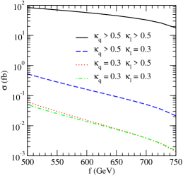
Figure 12: Total cross section for $e^{+}e^{-}\to W_{H}^{+}W_{H}^{-}\to A_{H}A_{H}jjjj$ at the LC. 

IV.1 Mass measurement of $W_{H}$

In order to simulate the detector acceptance, we require the transverse momentum ($p_{T}^{j}$) and rapidity ($\eta^{j}$) of all the final state jets to satisfy the following basic cuts

$$p_{T}^{j}>15\,{\rm GeV},\qquad\left|\eta^{j}\right|<3\,.$$

We also demand that the four jets are resolvable as separated objects, i.e. requiring the separation in $\Delta R\equiv\sqrt{(\delta\eta)^{2}+(\delta\phi)^{2}}$ between any two jets to be larger than 0.4, where $\delta\eta$ and $\delta\phi$ denotes the separation in the rapidity and azimuthal angles, respectively. In order to reconstruct the two $W$ bosons, one need to isolate the four jets coming from the $W$ boson decay. Unfortunately, one cannot tell the jets apart experimentally because the information of quark’s charge and flavor is lost in the hadronization of the light quarks. In order to measure $m_{W_{H}}$, one needs to reconstruct the two $W$ bosons, i.e. finding out which two jets come from which $W$ boson. In this study we use the $W$ boson mass as a constraint to reconstruct two $W$ bosons:

• In order to identify the jets, we order the four jets by their transverse momentum,

  $$p_{T}^{j_{1}}\geq p_{T}^{j_{2}}\geq p_{T}^{j_{3}}\geq p_{T}^{j_{4}}.$$ (17)

• We loop over all combinations of the four jets, i.e. ($j_{1}j_{2}$, $j_{3}j_{4}$), ($j_{1}j_{3}$, $j_{2}j_{4}$) and ($j_{1}j_{4}$, $j_{2}j_{3}$), and calculate the invariant masses of the reconstructed $W$ bosons. We then calculate the deviations from the true $W$ boson mass ($m_{W}$) for each combination,

  $$\Delta=\sqrt{\left(m_{1}(jj)-m_{W}\right)^{2}+\left(m_{2}(jj)-m_{W}\right)^{2}},$$ (18)

  and select the combination giving rise to the minimal deviations to reconstruct the $W$ bosons. Although the efficiency of the $W$ boson reconstruction procedure is very high ($\sim 99.1\%$), we cannot distinguish the two reconstructed $W$ bosons because the charge information is lost. But as to be shown below, we do not need the information of the $W$ boson charge to determine the mass and spin of $W_{H}$. Just for bookmark we denote the $W$ boson consisting the highest $p_{T}$ jet as $W_{1}$ while the other $W$ boson as $W_{2}$.

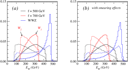
Figure 13: Normalized energy distributions of the reconstructed $W$ bosons for $\kappa_{q}=1$ at the LC. 

In Fig. 13, we present the energy distributions of the reconstructed $W$ bosons ($E_{W}$) where the energy of $W_{1}$ ($E_{W_{1}}$) peaks in the large energy region while the energy of $W_{2}$ ($E_{W_{2}}$) in the small energy region. The asymmetry between $W_{1}$ and $W_{2}$ is due to our requirement that the $W_{1}$ boson includes the leading-$p_{T}$ jet. Since the $A_{H}$ bosons are massive, the $E_{W}$ distributions exhibit sharp drops in both small and large energy regions, which can be used to measure the masses of $W_{H}$ and $A_{H}$ Kong and Park (2007). The ending points of the energy distribution of the $W$ boson are given by

$$E_{\pm}=\gamma\left(E_{W}^{\star}\pm\beta\,p_{W}^{\star}\right),$$ (19)

where $\beta=\sqrt{1-4m_{W_{H}}^{2}/s}$, $\gamma=1/\sqrt{1-\beta^{2}}$ and $E_{W}^{\star}$($p_{W}^{\star}$) is the energy (momentum) magnitude of the $W$ boson in the rest frame of $W_{H}$,

$$E_{W}^{\star} = \frac{m_{W_{H}}^{2}-m_{A_{H}}^{2}+m_{W}^{2}}{2m_{W_{H}}},$$ (20)

$$p_{W}^{\star} = \frac{\sqrt{\left[m_{W_{H}}^{2}-\left(m_{A_{H}}+m_{W}\right)^{2}\right]\left[m_{W_{H}}^{2}-\left(m_{A_{H}}-m_{W}\right)^{2}\right]}}{2m_{W_{H}}}.$$ (21)

From $E_{\pm}$ we can derive $m_{W_{H}}$ and $m_{A_{H}}$ as follows:

$$m_{W_{H}} = \sqrt{\frac{s}{2}}\frac{\sqrt{E_{+}E_{-}}}{E_{+}+E_{-}}\sqrt{1+\frac{m_{W}^{2}}{E_{+}E_{-}}+\sqrt{\left(1-\frac{m_{W}^{2}}{E_{+}^{2}}\right)\left(1-\frac{m_{W}^{2}}{E_{-}^{2}}\right)}},$$ (22)

$$m_{A_{H}} = m_{W_{H}}\sqrt{1-\frac{2\left(E_{+}+E_{-}\right)}{\sqrt{s}}+\frac{m_{W}^{2}}{m_{W_{H}}^{2}}}.$$ (23)

In this study, we choose two sample points: (1) $m_{W_{H}}=320\,{\rm GeV}$ and $m_{A_{H}}=66\,{\rm GeV}$ for $f=500\,{\rm GeV}$; (2) $m_{W_{H}}=450\,{\rm GeV}$ and $m_{A_{H}}=101\,{\rm GeV}$ for $f=700\,{\rm GeV}$. Hence, for the former sample point, $E_{+}=426\,{\rm GeV}$ and $E_{-}=85\,{\rm GeV}$, while for the latter sample point, $E_{+}=345\,{\rm GeV}$ and $E_{-}=146\,{\rm GeV}$. The small tails of the lower and higher ending points are due to the width effects of $W_{H}$ and $W$. After reading out the ending points from the $E_{W}$ distribution, one can determine $m_{W_{H}}$ and $m_{A_{H}}$ from Eqs. (22) and (23). The accuracy of this method highly depends on how well one can reconstruct the $W$ boson momentum and how well one can determine the ending points. Furthermore, the collider detection is not perfect. In order to mimic the finite detection efficiency of the detector, we smear the momenta of all the final state jets by a Gaussian distribution with

$$\frac{\Delta E}{E}=\frac{50\%}{\sqrt{E}},$$ (24)

where $E$ is the energy of the observed parton and the resolution of the energy measurement is assumed to be $50\%\sqrt{E}$. The $E_{W}$ distributions after energy smearing are shown in Fig. 13(b). We note that the shapes of the distributions of both signal and background are changed slightly, but the positions of the ending points remain almost the same, which lead to $4\%$ and $8\%$ error in the mass measurements of $W_{H}$ and $A_{H}$ for $f=700$ GeV, respectively.

IV.2 Spin correlations

Although one can derive the $W_{H}$ mass by using $E_{+}$ and $E_{-}$ from the $E_{W}$ distributions, one still needs to verify that such a signal indeed comes from the LHT and not from other new physics models. For example, the minimal supersymmetric extension of the standard model (MSSM) with R-parity can also have exactly the same collider signature ($4j+\not\!\!E_{T}$) from the process

$$e^{+}e^{-}\to\widetilde{W}^{+}\widetilde{W}^{-}\to\tilde{\gamma}\tilde{\gamma}W^{+}(\to jj)W^{-}(\to jj),$$

where the photino ($\tilde{\gamma}$) is assumed to be the lightest SUSY particle which plays as the dark matter candidate. Obviously, examining the kinematics distributions is not sufficient to discriminate the LHT from the MSSM. Below we will show that the spin correlation between the $W$ boson and its mother particle is a good tool to tell these two models apart. Taking advantage of the known c.m. energy of the LC, one can reconstruct the kinematics of the two missing $A_{H}$ bosons and in turn study the spin correlation effects for model discrimination. Details of the event reconstruction are shown in the Appendix. Below, we only present our results of the phenomenological study.

Table 2: Efficiencies of the $A_{H}$ reconstruction after requiring $\mathbb{C}^{2}>0$.

$f$ (GeV)		input (GeV)			no smearing				with smearing
		$m_{W_{H}}$	$m_{A_{H}}$		signal		BKGD		signal		BKGD
500		317	66		$87\%$		$0.5\%$		$80\%$		$1.4\%$
600		384	84		$90\%$		$0.3\%$		$82\%$		$0.7\%$
700		450	101		$89\%$		$0.1\%$		$79\%$		$0.3\%$

After event reconstruction, we denote $A_{H1}$ as the reconstructed $A_{H}$ boson associated with $W_{1}$ while $A_{H2}$ as the one with $W_{2}$. The inequality $\mathbb{C}^{2}>0$ (cf. Eq. 43), has to be satisfied in order to reconstruct the momentum of $A_{H}$’s. Since $\mathbb{C}^{2}$ depends on $m_{W_{H}}$ and $m_{A_{H}}$, inputting the correct masses of $W_{H}$ and $A_{H}$ will significantly enhance the efficiency of the event reconstruction. Furthermore, it is easy to show that the dependence of $\mathbb{C}^{2}$ upon $m_{W_{H}}$ is much stronger than the one upon $m_{A_{H}}$. Hence, if one inputs the correct $m_{W_{H}}$, then one may reach the maximal reconstruction efficiency. The reconstruction efficiencies are summarized in Table 2 where we consider both cases of with and without detector smearing effects. The detector effects reduce the efficiency of the signal reconstruction about $10\%$ but increase the efficiency of the background reconstruction by a factor $2\sim 3$.

Using the known kinematics of the $A_{H}$ bosons, we can reconstruct the momentum of the $W_{H}$ bosons. We then can plot the $\cos\theta^{*}$ distribution of the $W$ boson in Fig. 14 where $\theta^{\ast}$ is the angle between $W$ boson and $W_{H}$ boson in the rest frame of $W_{H}$ boson. The left figure shows the true $\cos\theta^{*}$ distribution where we assume all the particles in the final state, including the $A_{H}$ bosons, are perfectly tagged. The right figure shows the $\cos\theta^{*}$ distributions after the $W$ boson reconstruction. The distributions can be understood as follows. In the LHT, the decay products of the $W_{H}$ boson, $W$ and $A_{H}$, are highly boosted because $W_{H}$ is much heavier than $A_{H}$ and $W$. Then the $A_{H}$ and $W$ bosons would be predominately in the longitudinal polarization states. Therefore, the decay of $W_{H}\to A_{H}W$ could be treated as a vector boson decaying into two scalars. Due to the angular momentum conservation, the spacial function of $A_{H}$ and $W_{H}$ would be dominated by p-wave ($\sim\sin^{2}\theta^{\ast}$), as shown in Fig. 14 (a). Duo to the $W$ boson reconstruction, cf. Fig 13, $W_{1}$, the $W$ boson containing the leading jet, moves parallel with the $W_{H}$ and thus peaks in the forward direction while $W_{2}$ peaks in the backward direction.

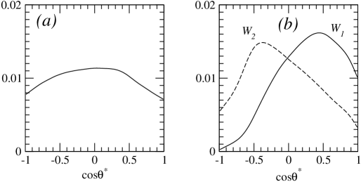
Figure 14: Normalized distribution of $\cos\theta^{*}$, where $\theta^{*}$ is the angle between the $W$ boson and its mother particle $W_{H}$ in the rest frame of $W_{H}$ for $f=500$ GeV: (a) true distribution; (b) after the $W$ boson reconstruction. 

How could we use this angular correlation to distinguish different models? Let us consider the signature of $W^{+}W^{-}$+ $\not\!\!E_{T}$ which is generated by two heavy vector bosons in the LHT. That signature could also be induced by many other new physics models:

• It can come from the decays of a heavy scalar ($\Phi$) pair, e.g. $e^{+}e^{-}\to\Phi\Phi\to W^{+}W^{-}+VV$, and the missing particle ($V$) must be a vector boson. Due to the scalar decay, the $\cos\theta^{*}$ distribution should be flat, cf. the red dotted curve in Fig. 15(a).

• It can also come from the decays of a heavy fermion ($\mathcal{F}$) pair, e.g. $e^{+}e^{-}\to\mathcal{F}\mathcal{F}\to W^{+}W^{-}+\chi\chi$, and the missing particle ($\chi$) must also be a fermion. It is well know that the $\cos\theta^{*}$ distribution should be in the form of $1-\cos\theta^{*}$, $1+\cos\theta^{*}$, or the combination of them. Here we plot the first two distributions in Fig. 15(a), cf. the blue dashed and green dashed curves .

The distinctive difference in the true $\cos\theta^{*}$ distributions will be affected by the $W$ boson reconstruction, but the predictions from different models are still distinguishable, cf. Fig. 15(b) and (c).

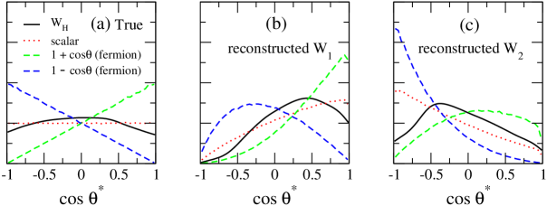
Figure 15: Normalized $\cos\theta^{*}$ distributions for different spin particles: (a) the true distribution while (b) and (c) are the distributions after $W$ boson reconstruction. 

V Conclusion 

In this paper we study the collider phenomenologies of the $W_{H}$ pair production in the LHT at the LHC and the LC. The $W_{H}$ pair production is of particular importance in the LHT because the mass of $W_{H}$ is proportional to the symmetry breaking scale $f$. One thus can unambiguously determine $f$ by measuring $m_{W_{H}}$.

At the tree level, the $W_{H}$ boson pair can be produced either via the $s$-channel process with the photon and $Z$ boson exchanged or via the $t$-channel process with a T-odd fermion exchanged. The total cross section highly relies on the mass of the T-odd fermion. Although the $s$-channel and $t$-channel contributions are both constructive, their interference effects are destructive. The total cross section reaches the minimum when the $s$-channel and $t$-channel contributions are comparable. Once being produced, the $W_{H}$ boson will decay into a T-odd particle and a T-even SM particle. The decay pattern of the $W_{H}$ boson is determined by the masses of other new physics particles such as $A_{H}$, $\ell_{-}$ and $q_{-}$ (we assume $A_{H}$ being the lightest T-odd particle):

1. If $W_{H}$ is the second lightest T-odd particle, it can only decay into $A_{H}W$.

2. If $W_{H}$ is heavier than $\ell_{-}$ and/or $q_{-}$, it will decay into $\ell\ell_{-}$ and/or $qq_{-}$ as well as $A_{H}W$.

In this work we treat the $\kappa_{q}$ and $\kappa_{\ell}$ separately. In order to avoid the FCNC problem, we further demand $\kappa_{q}$ and $\kappa_{\ell}$ being diagonal in the flavor space.

To avoid the huge QCD background at the LHC, we require the $W_{H}$ boson decay leptonically. Hence, the signal events can come either from the process in Eq. (11) for $\kappa_{\ell}=0.5$ or from the process in Eq. (12) for $\kappa_{\ell}=0.3$. We perform a Monte Carlo analysis of the signal process along with the SM backgrounds and find that the $W_{H}$ boson decaying leptonically, leading to a $\ell^{+}\ell^{\prime-}\not\!\!E_{T}$ signature, is very promising at the LHC. We apply the kinematical cuts in Eqs. (13, 14) and show the resulting significance contour in the plane of $\kappa_{q}$ and $\kappa_{\ell}$ in Fig. 10. We find that $f$ can be probed up to $750\,{\rm GeV}$ for $\kappa_{\ell}=0.5$ or $1\,{\rm TeV}$ for $\kappa_{\ell}=0.3$ at the $5\sigma$ level with an integrated luminosity of $100\,{\rm fb}^{-1}$. It is worth mentioning that $f$ can be probed up to the same limits at the $95\%$ C.L. even at low luminosity ($\mathcal{L}=10\,{\rm fb}^{-1}$) LHC operation. Although the two processes given in Eqs. (11, 12) give rise to the exactly same collider signature, they can be further discriminated in the distributions of the transverse momentum and energy of the final state charged leptons, see Fig. 11. However, the $W_{H}$ boson mass still cannot be determined at the LHC due to the four missing particles in the final state.

In order to determine the mass and spin of the $W_{H}$ boson, we perform a Monte Carlo study of the $W_{H}$ pair production at the LC. Owing to the clean background at the LC, we are able to search the $W_{H}$ boson using its hadronic decay mode which leads to a $4j+\not\!\!E_{T}$ signature generated from Eq. (15). Due to the known center-of-mass energy at the LC, the masses of $W_{H}$ and $A_{H}$ can be determined from the ending points of the energy distributions of the two reconstructed $W$ bosons. For example, one can measure the mass of $W_{H}$ ($A_{H}$) within an error of $4\%$ ($8\%$) for $f=700\,{\rm GeV}$, respectively, even after including the detector smearing effects. Following the study of the $W^{+}W^{-}$ pair production at the LEP Hagiwara et al. (1987), we present an algorithm of reconstructing the kinematics of two undetectable $A_{H}$ bosons. It enables us to study the spin correlation between the $W$ boson and its mother particle ($W_{H}$) which is a powerful tool to distinguish other new physics models from the LHT, as shown in Fig. 15.

Combining the studies of the $W_{H}^{+}W_{H}^{-}$ pair production at the LHC and LC, it is possible to determine or further constrain the parameter $f$, $\kappa_{q}$ and $\kappa_{\ell}$. In order to fix all the parameters of the LHT, direct search of other independent channels, e.g. top quark partners (both T-odd and T-even) pair production and T-odd fermions ( both leptons and quarks) pair production, must be included in a systematic way. One then can compare all these independent channels to check the consistence of the LHT.

Appendix A $A_{H}$ reconstruction at the LC

In this section we present an algorithm of determining the kinematics of $A_{H}$ at the LC. This algorithm has been proposed in the study of the $W$ boson at the LEP through the process $e^{+}e^{-}\to W^{+}W^{-}\to\ell^{+}\nu_{\ell}\ell^{\prime-}\bar{\nu}_{\ell^{\prime}}$ Hagiwara et al. (1987). The difficulty is attributed to the existence of two missing particles in the final state. The following kinematics analysis, presented below, shows that the two unobserved momenta of $A_{H}$ bosons can be determined from the reconstructed $W$ bosons up to a twofold discrete ambiguity, in the limit where the $W$- and $W_{H}$-width are neglected.

Here we consider the process

$$e^{+}e^{-}\to AA^{\prime},\,\,\,A\to BC,\,\,A^{\prime}\to B^{\prime}C^{\prime}$$ (25)

where $A(A^{\prime})$ is the mother particle while $B(B^{\prime})$ and $C(C^{\prime})$ are the decay products of the mother particles. Here we require $B(B^{\prime})$ is observable while $C(C^{\prime})$ undetectable. Furthermore, we assume

$$m_{A}=m_{A^{\prime}},\quad m_{C}=m_{C^{\prime}}.$$ (26)

One of the advantage of the LC is the known center-of-mass energy of the system. For example, the momentum of the incoming particles are

$$p_{e^{+}} = \left(\begin{array}[]{cccc}E_{t},&0,&0,&E_{t}\end{array}\right),$$ (28)

$$p_{e^{-}} = \left(\begin{array}[]{cccc}E_{t},&0,&0,&-E_{t}\end{array}\right),$$ (30)

where $E_{t}=\sqrt{S}/2$, where $\sqrt{S}$ is the total energy of the linear collider.

From the momentum conservation, we obtain

$$E_{A}=E_{B}+E_{C}, E_{A^{\prime}}=E_{B^{\prime}}+E_{C^{\prime}},$$ (31)

$$\vec{p}_{A}=\vec{p}_{B}+\vec{p}_{C}, \vec{p}_{A^{\prime}}=\vec{p}_{B^{\prime}}+\vec{p}_{C^{\prime}},$$ (32)

where $E_{i}(\vec{p}_{i})$ denotes the energy (three momentum) of the particle $i$, respectively. At the LC,

$$E_{A}=E_{A^{\prime}}=E_{t},\quad E_{C}=E_{t}-E_{B},\quad E_{C^{\prime}}=E_{t}-E_{B^{\prime}}.$$ (33)

From Eq. (32) and the on-shell conditions of the final state particles we obtain

$$2\vec{p}_{B}\cdot\vec{p}_{C} = E_{A}^{2}-m_{A}^{2}-\left(E_{B}^{2}-m_{B}^{2}\right)-\left(E_{C}^{2}-m_{C}^{2}\right),$$ (34)

$$2\vec{p}_{B^{\prime}}\cdot\vec{p}_{C^{\prime}} = E_{A^{\prime}}^{2}-m_{A^{\prime}}^{2}-\left(E_{B^{\prime}}^{2}-m_{B^{\prime}}^{2}\right)-\left(E_{C^{\prime}}^{2}-m_{C^{\prime}}^{2}\right).$$ (35)

Using the momentum conservation

$$\vec{p}_{B}+\vec{p}_{B^{\prime}}+\vec{p}_{C}+\vec{p}_{C^{\prime}}=0,$$ (36)

one obtains

$$2\vec{p}_{B^{\prime}}\cdot\vec{p}_{C}=\left(E_{C^{\prime}}^{2}-m_{C^{\prime}}^{2}\right)-\left(E_{A^{\prime}}^{2}-m_{A^{\prime}}^{2}\right)-\left(E_{B^{\prime}}^{2}-m_{B^{\prime}}^{2}\right)-2\vec{p}_{B}\cdot\vec{p}_{B}.$$ (37)

At last, the on-shell condition of particle $C$ gives us

$$\left|\vec{p}_{C}\right|^{2}=E_{C}^{2}-m_{C}^{2}.$$ (38)

Hence, one can determine $\vec{p}_{C}$ from Eqs. (34, 37, 38). We expand $\vec{p}_{C}$ in term of $\vec{p}_{B}$ and $\vec{p}_{B^{\prime}}$ as following

$$\vec{p}_{C}=\mathbb{A}\vec{p}_{B}+\mathbb{B}\vec{p}_{B^{\prime}}+\mathbb{C}\vec{p}_{B}\times\vec{p}_{B^{\prime}}.$$ (39)

Then one can derive $a$ and $b$ from Eqs. (34, 37)

$$\left(\begin{array}[]{c}\mathbb{A}\\ \mathbb{B}\end{array}\right)=\frac{1}{\left|\vec{p}_{B}\right|^{2}\left|\vec{p}_{B^{\prime}}\right|^{2}-\left(\vec{p}_{B}\cdot\vec{p}_{B^{\prime}}\right)^{2}}\left(\begin{array}[]{cc}\left|\vec{p}_{B^{\prime}}\right|^{2}&-\vec{p}_{B}\cdot\vec{p}_{B^{\prime}}\\ -\vec{p}_{B}\cdot\vec{p}_{B^{\prime}}&\left|\vec{p}_{B}\right|^{2}\end{array}\right)\left(\begin{array}[]{c}M\\ N\end{array}\right),$$ (40)

where

$$M \equiv \frac{1}{2}\left[E_{A}^{2}-m_{A}^{2}-\left(E_{B}^{2}-m_{B}^{2}\right)-\left(E_{C}^{2}-m_{C}^{2}\right)\right],$$ (41)

$$N \equiv \frac{1}{2}\left[\left(E_{C^{\prime}}^{2}-m_{C^{\prime}}^{2}\right)-\left(E_{A^{\prime}}^{2}-m_{A^{\prime}}^{2}\right)-\left(E_{B^{\prime}}^{2}-m_{B^{\prime}}^{2}\right)-2\vec{p}_{B}\cdot\vec{p}_{B}\right].$$ (42)

The remaining variable $\mathbb{C}$ is determined using Eq. (38):

$$\mathbb{C}^{2}=\frac{1}{\left|\vec{p}_{B}\times\vec{p}_{B^{\prime}}\right|^{2}}\left[E_{C}^{2}-m_{C}^{2}-\mathbb{A}^{2}\left|\vec{p}_{B}\right|^{2}-\mathbb{B}^{2}\left|\vec{p}_{B^{\prime}}\right|^{2}-2\mathbb{A}\mathbb{B}\vec{p}_{B}\cdot\vec{p}_{B^{\prime}}\right].$$ (43)

The sign of $\mathbb{C}$ cannot be determined. This explicitly exhibits a twofold discrete ambiguity. The inequality $\mathbb{C}^{2}>0$ is expected to be violated only by finite $W$- and $W_{H}$-width effects. Needless to say, using wrong $m_{C}$ and $m_{A}$ will lead to a negative $\mathbb{C}^{2}$ which can serve to measure $m_{A}$ and $m_{C}$ as mentioned earlier. In the exceptional case where the momenta of particle $B$ and $B^{\prime}$ are parallel, one obtains a one-parameter family of solution for which the azimuthal angle of $\vec{p}_{C}$ with respect to $\vec{p}_{B}$ is left undetermined.

References

- Arkani-Hamed et al. (2001) N. Arkani-Hamed, A. G. Cohen, and H. Georgi, Phys. Lett. B513, 232 (2001), eprint hep-ph/0105239.
- Schmaltz and Tucker-Smith (2005) M. Schmaltz and D. Tucker-Smith, Ann. Rev. Nucl. Part. Sci. 55, 229 (2005), eprint hep-ph/0502182.
- Perelstein (2007) M. Perelstein, Prog. Part. Nucl. Phys. 58, 247 (2007), eprint hep-ph/0512128.
- Arkani-Hamed et al. (2002) N. Arkani-Hamed, A. G. Cohen, E. Katz, and A. E. Nelson, JHEP 07, 034 (2002), eprint hep-ph/0206021.
- Csaki et al. (2003a) C. Csaki, J. Hubisz, G. D. Kribs, P. Meade, and J. Terning, Phys. Rev. D67, 115002 (2003a), eprint hep-ph/0211124.
- Csaki et al. (2003b) C. Csaki, J. Hubisz, G. D. Kribs, P. Meade, and J. Terning, Phys. Rev. D68, 035009 (2003b), eprint hep-ph/0303236.
- Hewett et al. (2003) J. L. Hewett, F. J. Petriello, and T. G. Rizzo, JHEP 10, 062 (2003), eprint hep-ph/0211218.
- Chen and Dawson (2004) M.-C. Chen and S. Dawson, Phys. Rev. D70, 015003 (2004), eprint hep-ph/0311032.
- Kilian and Reuter (2004) W. Kilian and J. Reuter, Phys. Rev. D70, 015004 (2004), eprint hep-ph/0311095.
- Han and Skiba (2005) Z. Han and W. Skiba, Phys. Rev. D71, 075009 (2005), eprint hep-ph/0412166.
- Cheng and Low (2003) H.-C. Cheng and I. Low, JHEP 09, 051 (2003), eprint hep-ph/0308199.
- Cheng and Low (2004) H.-C. Cheng and I. Low, JHEP 08, 061 (2004), eprint hep-ph/0405243.
- Low (2004) I. Low, JHEP 10, 067 (2004), eprint hep-ph/0409025.
- Hubisz et al. (2006) J. Hubisz, P. Meade, A. Noble, and M. Perelstein, JHEP 01, 135 (2006), eprint hep-ph/0506042.
- Hubisz and Meade (2005) J. Hubisz and P. Meade, Phys. Rev. D71, 035016 (2005), eprint hep-ph/0411264.
- Belyaev et al. (2006) A. Belyaev, C.-R. Chen, K. Tobe, and C. P. Yuan (2006), eprint hep-ph/0609179.
- Chen et al. (2006) C.-R. Chen, K. Tobe, and C. P. Yuan, Phys. Lett. B640, 263 (2006), eprint hep-ph/0602211.
- Choudhury et al. (2006a) S. R. Choudhury, A. S. Cornell, N. Gaur, and A. Goyal, Phys. Rev. D73, 115002 (2006a), eprint hep-ph/0604162.
- Blanke et al. (2006a) M. Blanke et al. (2006a), eprint hep-ph/0610298.
- Hundi et al. (2006) R. S. Hundi, B. Mukhopadhyaya, and A. Nyffeler (2006), eprint hep-ph/0611116.
- Cao et al. (2006) Q.-H. Cao, C. S. Li, and C. P. Yuan (2006), eprint hep-ph/0612243.
- Blanke et al. (2006b) M. Blanke et al., JHEP 12, 003 (2006b), eprint hep-ph/0605214.
- Blanke et al. (2007a) M. Blanke et al., Phys. Lett. B646, 253 (2007a), eprint hep-ph/0609284.
- Blanke et al. (2007b) M. Blanke, A. J. Buras, B. Duling, A. Poschenrieder, and C. Tarantino, JHEP 05, 013 (2007b), eprint hep-ph/0702136.
- Blanke et al. (2007c) M. Blanke, A. J. Buras, S. Recksiegel, C. Tarantino, and S. Uhlig (2007c), eprint hep-ph/0703254.
- Blanke et al. (2007d) M. Blanke, A. J. Buras, S. Recksiegel, C. Tarantino, and S. Uhlig (2007d), eprint arXiv:0704.3329 [hep-ph].
- Choudhury et al. (2006b) S. R. Choudhury, A. S. Cornell, A. Deandrea, N. Gaur, and A. Goyal (2006b), eprint hep-ph/0612327.
- Yue and Zhang (2007) C.-X. Yue and N. Zhang, Europhys. Lett. 77, 51003 (2007), eprint hep-ph/0609247.
- Chen et al. (2007) C.-S. Chen, K. Cheung, and T.-C. Yuan, Phys. Lett. B644, 158 (2007), eprint hep-ph/0605314.
- Hong-Sheng (2007) H. Hong-Sheng, Phys. Rev. D75, 094010 (2007), eprint hep-ph/0703067.
- Kai et al. (2007) P. Kai et al. (2007), eprint arXiv:0706.1358 [hep-ph].
- Wang et al. (2007) L. Wang, W. Wang, J. M. Yang, and H. Zhang (2007), eprint arXiv:0705.3392 [hep-ph].
- Yue et al. (2007) C.-X. Yue, N. Zhang, and S.-H. Zhu (2007), eprint arXiv:0707.0729 [hep-ph].
- Freitas and Wyler (2006) A. Freitas and D. Wyler, JHEP 11, 061 (2006), eprint hep-ph/0609103.
- Matsumoto et al. (2006) S. Matsumoto, M. M. Nojiri, and D. Nomura (2006), eprint hep-ph/0612249.
- Choudhury and Ghosh (2006) D. Choudhury and D. K. Ghosh (2006), eprint hep-ph/0612299.
- Carena et al. (2007) M. Carena, J. Hubisz, M. Perelstein, and P. Verdier, Phys. Rev. D75, 091701 (2007), eprint hep-ph/0610156.
- Stelzer and Long (1994) T. Stelzer and W. F. Long, Comput. Phys. Commun. 81, 357 (1994), eprint hep-ph/9401258.
- Maltoni and Stelzer (2003) F. Maltoni and T. Stelzer, JHEP 02, 027 (2003), eprint hep-ph/0208156.
- Pukhov (2004) A. Pukhov (2004), eprint hep-ph/0412191.
- Primack et al. (1988) J. R. Primack, D. Seckel, and B. Sadoulet, Ann. Rev. Nucl. Part. Sci. 38, 751 (1988).
- Yao et al. (2006) W. M. Yao et al. (Particle Data Group), J. Phys. G33, 1 (2006).
- Kong and Park (2007) K. Kong and S. C. Park (2007), eprint hep-ph/0703057.
- Hagiwara et al. (1987) K. Hagiwara, R. D. Peccei, D. Zeppenfeld, and K. Hikasa, Nucl. Phys. B282, 253 (1987).