The Effect of Noise Correlation in AF
Relay Networks

Abstract

In wireless relay networks, noise at the relays can be correlated possibly due to common interference or noise propagation from preceding hops. In this work we consider a parallel relay network with noise correlation. For the relay strategy of amplify-and-forward (AF), we determine the optimal rate maximizing relay gains when correlation knowledge is available at the relays. The effect of correlation on the performance of the relay networks is analyzed for the cases where full knowledge of correlation is available at the relays and when there is no knowledge about the correlation structure. Interestingly we find that, on the average, noise correlation is beneficial regardless of whether the relays know the noise covariance matrix or not. However, the knowledge of correlation can greatly improve the performance. Typically, the performance improvement from correlation knowledge increases with the relay power and the number of relays. With perfect correlation knowledge the system is capable of canceling interference if the number of interferers is less than the number of relays.

For a dual-hop multiple access parallel network, we obtain closed form expressions for the maximum sum-rate and the optimal relay strategy. The relay optimization for networks with three hops is also considered. For any relay gains for the first stage relays, this represents a parallel relay network with correlated noise. Based on the result of two hop networks with noise correlation, we propose an algorithm for solving the relay optimization problem for three-hop networks.

I Introduction

Wireless mesh networks where information is transferred via multiple hops and routes provide significant throughput enhancement and have been the focus of much recent work [1, 2, 3, 4]. Various relay strategies have been studied in literature [5, 6, 7]. These strategies include amplify-and-forward [8, 9], where the relay sends a scaled version of its received signal to the destination, demodulate-and-forward [9] in which the relay demodulates individual symbols and retransmits, decode-and-forward [7, 5] in which the relay decodes the entire message, re-encodes it and re-transmits it to the destination, and compress-and-forward [5, 6] where the relay sends a quantized version of its received signal. Among these strategies, amplify and forward has been found to be highly suitable for parallel relay networks for its ability to pass on soft information [10, 11, 12]. In one of the first works [13] on the parallel relay channel, it is shown that AF achieves the capacity cut-set bound at high relay power. In [4] it is shown that full degrees of freedom can be achieved with AF in a multi-hop parallel relay network where the hops are orthogonalized by design. There are numerous other examples in literature that corroborate the effectiveness of AF [14, 15, 16, 12, 17, 18, 19]. For an AF relay network, the relay design involves optimizing the relay amplification factors to maximize performance. Previous work pertaining to relay optimization for AF relay networks includes both single-user relaying [20, 21, 22, 23, 24, 25] and multi-user relaying [2, 26].

Most work in the literature [20, 27, 21, 22, 23, 26, 24, 25] assumes independent noise at the relay terminals. However, noise correlation between nodes occurs in wireless relay networks due to several reasons. In this paper we explore the effect of noise correlation for the following two models.

Figure 1: Noise correlation model 1:  Parallel relay network with common interference

1. Common Interference Model
   Due to the broadcast nature of wireless networks, the relays are exposed to a set of common interferers resulting in correlated noise at the nodes. As shown in Fig. 1, each relay in addition to its local noise observes common interference.

2. Noise propagation with multi-hop AF relaying (Three-hop model)
   Consider a three-hop network as shown in Fig. 2. If the first stage relays amplify their received signal, each relay in the second stage observes a linear combination of noise from the preceding stage relays along with its own local noise. This clearly results in correlated noise at the second-stage relays.

   Figure 2: Noise correlation model 2:  Three-hop parallel relay network

Both the above models are of considerable practical importance. The natural question is whether the relays can exploit the correlation structure to improve performance. In practice, learning correlation may result in network overheads. Whether such overheads are justified depends on the potential advantage of learning correlation. Thus, our goal in this work is to estimate the improvement in performance when perfect correlation knowledge is available at the relays. The optimal relay design in this case will have the following two objectives:

1. Increase signal power: The relay gains can be designed such that the copies of desired signal adds up in phase.

2. Reduce interference power: The relay gains may be chosen such that the common interference terms add out of phase.

In general, these objectives cannot be achieved simultaneously and the relay design can be expected to be a trade-off between the two objectives.

This paper also addresses the relay optimization problem for networks with three hops. Such a network is interesting as it combines multiple hops with multiple paths. The problem of routing in the traditional link based decode and forward involves selecting a relay at each hop that maximizes the end to end throughput between the original source and the final destination. If there are $N$ relays in each of the $M$ hops, the problem is to find the best route among $N^{(M-1)}$ routes. With AF, all the routes are utilized with priority for each route determined by the power allocation and phase equalization at each of the relays across multiple hops. As we can control the priority for the routes, optimizing relay gains may be viewed as soft-routing.

I-A Results

The main results of this paper are summarized below.

1. We obtain closed form solutions for the optimal relay amplification vector and the maximum sum rate for the network with correlated noise at the relays. This result generalizes the single-user relay optimization in [21, 20] and the multi-source relay optimization in [2] both of which assume independent and identically distributed (i.i.d.) noise at the relays.

2. We find that correlation, on the average, is always beneficial regardless of the presence or absence of correlation knowledge at the relays. This is true irrespective of the channel state information (CSI) at the relays.

3. We study the benefits of exploiting noise correlation at the relays. We compare the maximum sum rate without correlation knowledge (relays use optimal amplification factors based on uncorrelated noise assumption even if noise is correlated) versus capacity with correlation knowledge. The following key questions are answered: Does correlation help? Is the correlation knowledge more (or less) helpful as the number of relays increases? What is the effect of correlation as the power at the relays increases, and when the first hop/second hop becomes stronger? We also provide asymptotic results to characterize the impact of relay noise correlation.

4. We apply the results of two hop relay networks with correlated noise to solve the relay optimization problem for three-hop AF relay networks with independent noise processes at the relays. We also characterize the behavior of the three-hop network as the transmit power at any of the stages tends to $\infty$. When the first or the last stage power is very high, the network can be reduced to a two-hop channel. When both the first and last stage powers are high, the network can be reduced to a point to point MIMO channel with a single data stream.

I-B Notation

We use bold upper letters to denote matrices and bold lower letters to denote vectors. Further $(.)^{*}$, $(.)^{T}$, $(.)^{\dagger}$ stand for conjugation, transposition and Hermitian transposition, respectively. ${\bf a}\odot{\bf b}$ represents element wise multiplication of two vectors. ${\bf A}=\mbox{diag}({\bf a})$ denotes a diagonal matrix A that contains on its diagonals the elements of ${\bf a}$. $\mbox{det}(\bf A)$, $\mbox{Tr}(\bf A)$, $\lambda_{\max}({\bf A})$, and ${\bf v}_{\max}({\bf A})$ denote the determinant, trace, principal eigen-value, and principal eigen-vector of ${\bf A}$ respectively. $\bf A^{-\dagger}$ denotes the Hermitian transposition of $\bf A^{-1}$. ${\bf v}(i)$ denotes the $i^{th}$ element of the vector $\bf v$ while ${\bf A}_{ij}$ denotes the element in the $i^{th}$ row and $j^{th}$ column of the matrix $\bf A$. $\mathbb{E}$ stands for the expectation operator. ${\bf v}\sim\mathcal{CN}({\bf w},{\bf A})$ indicates $\bf v$ is a complex Gaussian column vector with $\mathbb{E}[{\bf v}]={\bf w}$ and $\mathbb{E}[{\bf vv^{\dagger}}]={\bf A}$.

This paper is organized as follows. In the next section we consider a two hop relay network with noise correlation and address the relay optimization problems for both single and multi-user scenarios. We analyze the impact of correlation in Section III. In Section IV we address the relay optimization problem for three-hop AF networks. We conclude with Section V.

II Two-hop parallel relay network with noise correlation

Figure 3: Two-hop single user parallel relay network

II-A System Model

We consider a two-hop parallel relay network as shown in Fig. 3. In this model, the source $S$ communicates to the destination $D$ through a set of $N$ half-duplex relays, $R_{i}$, $i=1...N$. The data transmission takes place in two time slots. In the first slot, the source transmits to the relays and in the second slot, all the relays simultaneously forward their received signal to the destination. Note that there is no direct link between the source and the destination. All the nodes are equipped with a single antenna. The $N\times 1$ channel between the source and the relays is $\bf f$ while $\bf g$ is the $N\times 1$ channel between the relays and the destination. The entries of $\bf f$ and $\bf g$ are independent and i.i.d. complex Gaussian random variables with zero mean and unit variance. The source has power $P$ and the relays have a total power of $P_{R}$. The relay received symbols during the first time slot are

$${\bf r}={\bf f}x+{\bf n_{R}}$$ (1)

where $x$ is the source transmitted signal with power $\mathcal{E}[|x|^{2}]=P$, and ${\bf n_{R}}\sim\mathcal{CN}({\bf 0,~{}K})$ is AWGN with the covariance matrix $\bf K$, given by

$${\bf K}=\mathbb{E}[{\bf n_{R}n_{R}^{\dagger}}].$$

In the second slot, the relay $R_{i}\}_{i=1}^{N}$ scales its received signal with a complex scaling factor $d_{i}$ and transmits to the destination. We collect the relay gain factors $d_{i}$ in an $N\times 1$ vector $\bf d$. Then the received signal at the destination can be expressed as

$$y={\bf d^{T}Gf}x+{\bf d^{T}Gn_{R}}+n_{D}$$ (2)

where ${\bf G}=\mbox{diag}({\bf g})$ and $n_{D}\sim\mathcal{CN}(0,1)$ is additive white Gaussian noise (AWGN). Further, we assume that there is no correlation between destination noise $n_{D}$ and the relay noise vector $\bf n_{R}$ as these noise processes occur at two different time slots. We denote this relay network with the shorthand notation $\mathfrak{R}_{2}(P,{\bf f},{\bf d},P_{R},{\bf g})$ where the subscript 2 indicates that the network consists of two hops. The sum power constraint of the relays can be expressed as

$${\bf d^{\dagger}}\left[\left({\bf ff^{\dagger}}P+{\bf K}\right)\odot{\bf I}\right]{\bf d}=P_{R}$$ (3)

where $\odot$ represents the Hadamard product or the element-wise multiplication. Note that there is a strict equality for the power constraint. This is because higher total relay transmit power is equivalent to lower noise power at the destination. Finally a word about the sum-power constraint. With individual power constraints, not all the relays may operate at full power [28]. Thus the total power expenditure at the relays may change depending on the channel conditions. With sum-power constraint relays use all the power. This is helpful in interference limited systems where the interference from the relays to other wireless links in the network needs to be estimated. And most importantly, the sum power constraint allows tractable analysis and useful insights can be obtained as a result of it.

II-B Relay Optimization

From the destination received signal in (2), the signal-to-noise-ratio (SNR) at the destination is given by

$$\mbox{SNR}=\frac{\left|{\bf d^{T}G}{\bf f}\right|^{2}P}{{\bf d^{T}GKG^{\dagger}d^{*}}+1}$$ (4)

and the corresponding transmission rate is $R=\log(1+\mbox{SNR})$. We seek to maximize the transmission rate with respect to the amplification vector ${\bf d}$ subject to the sum power constraint at the relays. The following theorem provides the optimal relay design and maximum achievable rate with amplify and forward relays in a two hop parallel relay network with noise correlation.

Theorem 1

The maximum achievable rate in the two-hop parallel AF relay network $\mathfrak{R}_{2}(P,{\bf f},{\bf d},P_{R},{\bf g})$ where the relay noise covariance matrix is $\bf K$, is given by

$$R^{\circ}=\log(1+\mbox{SNR}^{\circ})$$ (5)

$$\mbox{SNR}^{\circ}=PP_{R}({\bf f\odot g})^{\dagger}{\bf A^{-1}}({\bf f\odot g})$$ (6)

and the optimal relay amplification vector ${\bf d}^{\circ}$ is

$${\bf d}^{\circ}=\kappa\left({\bf A^{-1}(f\odot g)}\right)^{*}$$ (7)

where

$${\bf A}={\bf K\odot gg^{\dagger}}P_{R}+{\bf ff^{\dagger}}P\odot{\bf I+K\odot I}$$ (8)

and

$$\kappa^{2}=\frac{P_{R}}{({\bf f\odot g})^{\dagger}{\bf A^{-1}}\left[\left({\bf ff^{\dagger}}P+{\bf K}\right)\odot{\bf I}\right]{\bf A^{-\dagger}}({\bf f\odot g})}.$$ (9)

The proof is presented in the Appendix.

Remark

In the absence of correlation, $\bf A$ is diagonal and the phase of relay $R_{i}$ is such that it cancels the phase of the forward channel ${\bf g}(i)$ and the backward channel ${\bf f}(i)$. However, with noise correlation, ${\bf A}$ is not a diagonal matrix. Therefore the optimal relay gain may not co-phase the input signal as part of noise can be canceled with relay phase and gain adjustments.

II-C Properties of the optimal relay network

In this section, we consider the limiting properties of the optimal relaying scheme. The proofs are available in the Appendix.

1. Relay power $P_{R}\rightarrow\infty$:  When the relay power is high, the network is equivalent to a single-input-multiple-output (SIMO) system modeled by ${\bf y=f}x+{\bf n}$ where $\bf K$ is the noise covariance matrix at the multiple antenna receiver and $P$ is the transmit power of the single antenna transmitter. Its capacity is given by

   $$C=\log(1+{\bf f^{\dagger}K^{-1}f}P).$$ (10)

   Note that the system is independent of ${\bf g}$. Here $\bf d^{\circ}=\kappa(G^{-\dagger}K^{-1}f)^{*}$ achieves (10). When ${\bf K}$ is not invertible (or equivalently $\mbox{det}({\bf K})=0$), the capacity is infinite. This means that the effective noise at the destination can be completely eliminated regardless of the source transmission rate. For any relay gain vector, $\bf d$, the network is equivalent to a SIMO system with the receive combining vector given by $({\bf d\odot g})$.
   

2. Source power $P\rightarrow\infty$:  For the optimal ${\bf d}^{\circ}$, the network is equivalent to a MISO system represented by $y={\bf gx}+n$ where $n$ is unit variance AWGN. Its capacity is given by

   $$C=\log(1+{\bf g^{\dagger}g}P_{R}),$$ (11)

   which is independent of the relay noise covariance matrix $\bf K$. ${\bf d}(i)=\kappa{\bf g^{*}}(i)/{\bf f}(i)$ achieves (11) in the relay network. For a general $\bf d$, the relay network represents a multiple-input-single-output (MISO) system $y={\bf gx}+n$, with the beamforming vector $\bf\frac{(d\odot f)}{\sqrt{(d\odot f)^{\dagger}(d\odot f)}}$ and transmit power equal to $P_{R}$.
   

3. Singular $\bf K$ or $\mbox{det}({\bf K})=0$:  Singular $\bf K$ in any of the noise correlation models of common interference and three-hop network may be unrealistic as the relays have independent local noise components. However the case of singular $\bf K$ provides useful insights when the power of the interference is very high for the common interference model, and when the total power of the first stage relays is very high in the three-hop model. Notice that the rank of $\bf K$ indicates the number of independent noise sources at the relays. Thus for singular $\bf K$ at most ($N-\mbox{rank}({\bf K})$) noise terms can be canceled with appropriate relay gains. Due to destination noise, the capacity of the relay network is finite even when $\bf K$ is singular.

The relay optimization result of Theorem 1 can be extended to several multi-user scenarios. As an example we consider the multiple access relay channel in the following.

II-D Extension: Multiple access parallel relay network with noise correlation

Consider a multi-source parallel relay network as shown in Fig. 4. In this model, $L$ source nodes wish to communicate to a common destination with the assistance of $N$ AF relays. In the first slot all the sources transmit. The relay received signals are given by

$${\bf r}=\sum_{i=1}^{L}{\bf f}_{i}x_{i}+{\bf n_{R}}$$ (12)

where $x_{i}$ is the signal transmitted by the $i^{th}$ source whose power is $\mathbb{E}[|x_{i}|^{2}]=P_{i}$. As in the single user case, the relays scale their received signal and transmit to the destination in the second slot. The received signal at the destination can be expressed as

$$y=\sum_{i=1}^{L}{\bf d^{T}Gf}_{i}x_{i}+{\bf d^{T}Gn_{R}}+n_{D}$$ (13)

The following theorem provides the maximum achievable sum rate and the optimal relay design.

Figure 4: Two-hop multi-source parallel relay network

Theorem 2

The maximum achievable sum rate in a two-hop multi-source parallel AF relay network with noise correlation is given by

$$R^{\circ}=\log(1+\mbox{SNR}^{\circ})$$ (14)

$$\mbox{SNR}^{\circ}=P_{R}\lambda_{\max}\left[{\bf A^{-1}B}\right]$$ (15)

and the optimal relay amplification vector $\bf d_{\Sigma}^{\circ}$ is

$${\bf d_{\Sigma}^{\circ}}=\kappa\left({\bf v_{\max}\left[A^{-1}B\right]}\right)^{*}$$ (16)

where

$${\bf A}={\bf K\odot gg^{\dagger}}P_{R}+\sum_{k=1}^{L}{\bf f_{k}f_{k}^{\dagger}}P_{k}\odot{\bf I+K\odot I}$$ (17)

$${\bf B}=\sum_{k=1}^{L}{\bf(f_{k}\odot g)(f_{k}\odot g)^{\dagger}}P_{k}$$ (18)

and $\kappa$ ensures compliance with the relay power constraint.

Refer to the Appendix for the proof. Since our principal goal is to investigate the effect of correlation in a single user parallel relay network, the rest of the paper will focus only on the single-user case.

III Does Correlation Help?

In this section, we address the following important questions:

1. Does correlation help when the relays know the covariance matrix?

2. Does correlation hurt when the relays are unaware of it?

To answer the first question we compare the following two scenarios.

• The noise is correlated and relays are aware of the correlation. (Scheme-11)

• The noise is uncorrelated. (Scheme-00)

To answer the second question we compare the following two scenarios.

• The noise is correlated and relays are unaware of the correlation. (Scheme-10)

• The noise is uncorrelated. (Scheme-00)

If Scheme-11 outperforms Scheme-00 then we can say that correlation helps if the relays are aware of it. Similarly, if Scheme-00 outperforms Scheme-10 then we can say that correlation hurts when the relays are unaware of it.

III-A Benchmark Schemes

III-A1 Relays with uncorrelated noise: Scheme-00

This setup has been commonly studied in literature [20, 21, 2, 24]. The system model consists of a two hop parallel relay network with independent noise at the relays. The noise covariance matrix, which is diagonal, is given by $\bf K\odot I$. For a sum power constraint at the relays, the optimum relay amplification vector is found in [21, 20]. The result can also be obtained from Theorem 1 by replacing $\bf K$ with $\bf K\odot I$. We thus obtain

$${\bf d}_{00}=\kappa\left[({\bf GKG^{\dagger}}P_{R}+{\bf ff^{\dagger}}P+{\bf K})\odot{\bf I}\right]^{-1}({\bf f^{\dagger}\odot g^{\dagger}})^{T}.$$ (19)

The SNR achieved at the destination with the optimal relay gain ${\bf d}_{00}$ is given by

$$\mbox{SNR}_{00}=PP_{R}{\bf(f\odot g)^{\dagger}}\left[({\bf GKG^{\dagger}}P_{R}+{\bf ff^{\dagger}}P+{\bf K})\odot{\bf I}\right]^{-1}{\bf(f\odot g)}.$$ (20)

A special case of Scheme-00 is where the relay noise terms are independent and identically distributed. Since we require the trace of the noise covariance matrix to be equal in all the schemes, the covariance matrix for this scheme will be

$${\bf K_{\mbox{iid}}}=\frac{\mbox{Tr({\bf K})}}{N}{\bf I}.$$

We denote this model as Scheme-iid indicating that the relay noise terms are i.i.d. Again, the optimal relay amplification vector for this model can be obtained from Theorem 1 by replacing $\bf K$ with $\frac{\mbox{Tr({\bf K})}}{N}{\bf I}$. Thus we have

$${\bf d}_{\mbox{iid}}=\kappa\left[\left({\bf GG^{\dagger}}\frac{\mbox{Tr({\bf K})}}{N}P_{R}+{\bf ff^{\dagger}}P+{\frac{\mbox{Tr({\bf K})}}{N}}{\bf I}\right)\odot{\bf I}\right]^{-1}({\bf f^{\dagger}\odot g^{\dagger}})^{T}.$$ (21)

The corresponding SNR is given by

$$\mbox{SNR}_{\mbox{iid}}=PP_{R}{\bf(f\odot g)^{\dagger}}\left[\left({\bf GG^{\dagger}}\frac{\mbox{Tr({\bf K})}}{N}P_{R}+{\bf ff^{\dagger}}P+{\frac{\mbox{Tr({\bf K})}}{N}}{\bf I}\right)\odot{\bf I}\right]^{-1}{\bf(f\odot g)}.$$ (22)

III-A2 Relays with no correlation knowledge: Scheme-10

In this scheme, correlation is induced between the relay noise terms. However the marginals remain the same as in Scheme-00, $n_{r_{i}}\sim\mathcal{CN}(0,{\bf K}_{ii})$; i.e. noise at relay $R_{i}$ is AWGN with variance ${\bf K}_{ii}$. Note that ${\bf K}_{ij}$ represents the correlation between the noise terms $n_{R_{i}}$ and $n_{R_{j}}$ for $i\neq j$, and in general may not be equal to zero. Since the relays do not utilize the correlation structure, the relay amplification vector is the same as in the case of Scheme-00, i.e.,

$${\bf d}_{10}={\bf d}_{00}.$$

The SNR achieved with the relay gain ${\bf D}_{10}=\mbox{diag}({\bf d}_{10})$ is given by

$$\mbox{SNR}_{10}=\frac{\left|{\bf(f\odot g)^{\dagger}}{\bf D}_{10}^{-1}{\bf(f\odot g)}\right|^{2}PP_{R}}{{\bf(f\odot g)^{\dagger}}{\bf D}_{10}^{-1}{\bf A}{\bf D}_{10}^{-1}(\bf f\odot g)}.$$ (23)

As there is no correlation knowledge at the relays, the relay operation here involves only co-phasing of the input signal and does not involve noise cancelation. It is straightforward to see that Scheme-11 will perform better than Scheme-10 as it exploits the correlation structure in designing the relay amplification factors. Rewriting the results from Theorem 1, the optimal relay amplification vector that exploits full correlation knowledge is

$${\bf d}_{11}=\kappa\left(\left[({\bf GKG^{\dagger}}P_{R}+{\bf ff^{\dagger}}P+{\bf K})\right]^{-1}({\bf f\odot g})\right)^{*}.$$ (24)

and the SNR achieved with $\bf d_{11}$ is given by

$$\mbox{SNR}_{11}=PP_{R}{\bf(f\odot g)^{\dagger}}\left({\bf GKG^{\dagger}}P_{R}+{\bf ff^{\dagger}}P+{\bf K}\right)^{-1}{\bf(f\odot g)}.\\$$ (25)

It is not clear whether Scheme-10 is also inferior to Scheme-00 and Scheme-iid. It is also not clear which is better among Scheme-00 and Scheme-iid. Answering these questions will provide useful insights into the impact of correlation in multi-hop AF relay networks. We address this in the rest of this section.

III-B Asymptotic analysis

We compare the schemes for the two extreme cases of $P_{R}\rightarrow\infty$ and $P\rightarrow\infty$.

III-B1 Relay Power $P_{R}\rightarrow\infty$

From the property of the optimal network at high $P_{R}$, we have from (10)

$$\mbox{SNR}_{11}={\bf f^{\dagger}K^{-1}f}P.$$ (26)

At very high $P_{R}$, ${\bf D_{10}}={\bf G(K\odot I)G^{\dagger}}P_{R}$ and ${\bf A}={\bf GKG^{\dagger}}P_{R}$ . Substituting these in (23), we obtain

$$\mbox{SNR}_{10} = \frac{\left|{\bf(f\odot g)}^{\dagger}({\bf G(K\odot I)G^{\dagger}}P_{R})^{-1}{\bf(f\odot g)}\right|^{2}PP_{R}}{{\bf(f\odot g)}^{\dagger}({\bf G(K\odot I)G^{\dagger}}P_{R})^{-1}({\bf GKG^{\dagger}}P_{R})({\bf G(K\odot I)G^{\dagger}}P_{R})^{-1}{\bf(f\odot g)}}$$ (27)

$$= \frac{{\bf(f^{\dagger}(K\odot I)^{-1}f)^{2}}P}{{\bf f^{\dagger}(K\odot I)^{-1}K(K\odot I)^{-1}f}}.$$ (28)

It is evident from (20) that the SNR of Scheme-11 at very high relay power is

$$\mbox{SNR}_{00} = P{\bf f}^{\dagger}{\bf(K\odot I)^{-1}}{\bf f}.$$ (29)

Similarly the SNR of Scheme-iid is readily obtained as

$$\mbox{SNR}_{\mbox{iid}} = \frac{{\bf f}^{\dagger}{\bf f}P}{\mbox{Trace}({\bf K})/N}.$$ (30)

Remark

Except for Scheme-10, all the relay schemes turn out to be a point to point SIMO channel. It must be noted that the noise at the multiple antenna receiver is correlated and the noise covariance matrix is the same as the relay noise covariance matrix of the original network. For Scheme-10, the multiple antenna receiver is unaware of the noise correlation and assumes the noise covariance matrix to be $\bf K\odot I$ instead of $\bf K$.

To answer the question whether correlation hurts when there exists no knowledge of it, let us consider the difference $\mbox{SNR}_{10}-\mbox{SNR}_{00}$. For the simple case of $N=2$ and for real channels, we have

$$\mbox{SNR}_{10}-\mbox{SNR}_{00}=\frac{-2{f}_{1}{f}_{2}{\bf K}_{12}({f}_{1}^{2}{\bf K}_{11}+{f}_{2}^{2}{\bf K}_{22})}{{f}_{1}^{2}{\bf K_{11}}+{f}_{2}^{2}{\bf K}_{22}+2{f}_{1}{f}_{2}{\bf K}_{12}}$$ (31)

where ${\bf f}=\left[f_{1}~{}f_{2}\right]^{T}$. The difference can be either positive or negative depending on the term $-2{f}_{1}{f}_{2}{\bf K}_{12}$. For example, when the signals are positively correlated (${f}_{1}{f}_{2}\geq 0$) and the noise components are negatively correlated ${\bf K}_{12}\leq 0$, then correlation helps as part of noise gets canceled. Similarly when both the signal and noise components are correlated in the same direction (positive or negative) then correlation hurts as it increases the noise power. Therefore the overall effect of correlation can only be determined from the average behavior.

Theorem 3

At high relay power $P_{R}$, Scheme-10 outperforms Scheme-00 in terms of both average SNR and average rate. That is

$$\mathbb{E}[\mbox{SNR}_{10}]\geq\mathbb{E}[\mbox{SNR}_{00}]~{}~{}\mbox{and}~{}~{}\mathbb{E}[\mbox{R}_{10}]\geq\mathbb{E}[\mbox{R}_{00}]$$

where $\mbox{R}_{10}=\log(1+\mbox{SNR}_{10})$ and $\mbox{R}_{00}=\log(1+\mbox{SNR}_{00})$.

The proof is presented in the Appendix.

The above result is significant as it suggests that, in the average sense, correlation does not hurt even if correlation knowledge is not available. To determine the relationship for the rest of the cases, we take the expectation of SNR in (26), (29), and (30):

$$\mathbb{E}[\mbox{SNR}_{11}] = P\sum_{i=1}^{N}\mathbb{E}[|{f}_{i}|^{2}](1/\lambda_{i})=P\sum_{i=1}^{N}1/\lambda_{i}$$ (32)

$$\mathbb{E}[\mbox{SNR}_{00}] = P\sum_{i=1}^{N}\mathbb{E}[|{f}_{i}|^{2}](1/{\bf K}_{ii})=P\sum_{i=1}^{N}1/{\bf K}_{ii}$$ (33)

$$\mathbb{E}[\mbox{SNR}_{\mbox{iid}}] = \frac{P\sum_{i=1}^{N}\mathbb{E}[|{f}_{i}|^{2}]}{\sum_{i=1}^{N}{\bf K}_{ii}/N}=\frac{NP}{\sum_{i=1}^{N}{\bf K}_{ii}/N}$$ (34)

where $\mathbb{E}[|{f}_{i}|^{2}]=1$ while $\lambda_{i}$ and ${\bf K}_{ii}$ are the $i^{th}$ eigen-value and $i^{th}$ main-diagonal term of ${\bf K}$ respectively. $\mathbb{E}[\mbox{SNR}_{11}]$ is greater than $\mathbb{E}[\mbox{SNR}_{00}]$ follows from the reason that the ordered vector containing the eigen-values of ${\bf K}$ majorizes the main diagonal of ${\bf K}$, i.e. ${\bf\lambda\succeq d}$. We also have $\mathbb{E}[\mbox{SNR}_{00}]\geq\mathbb{E}[\mbox{SNR}_{\mbox{iid}}]$ due to the harmonic-arithmetic mean inequality. Therefore we obtain the following relationship:

$$\mathbb{E}[\mbox{SNR}_{11}]\geq\mathbb{E}[\mbox{SNR}_{10}]\geq\mathbb{E}[\mbox{SNR}_{00}]\geq\mathbb{E}[\mbox{SNR}_{\mbox{iid}}]$$ (35)

Thus in the high relay power regime, correlation does not hurt even when the system is ignorant of the underlying noise correlation structure. Importantly, it is also clear that there is a performance gain when the correlation structure is exploited.

III-B2 Source Power $P\rightarrow\infty$

At very high source power, the optimal relay network (Scheme-11) is equivalent to a MISO system. From (11), we have

$$\mbox{SNR}_{11}=P_{R}{\bf g}^{\dagger}{\bf g}.$$ (36)

Similarly, it can be shown that the rest of the schemes also achieve the SNR in (36) at high $P$.

$$\mbox{SNR}_{10}=\mbox{SNR}_{00}=\mbox{SNR}_{\mbox{iid}}=P_{R}{\bf g}^{\dagger}{\bf g}.$$ (37)

It can be noticed that this scenario represents the maximal ratio transmission (MRT) where the relays act as a multiple antenna transmitter. This is intuitive as the noise at the relays is negligible compared to the source power and therefore the effect of the noise covariance matrix is non-existent. We now verify the results with numerical analysis in the following subsection.

III-C Numerical Results

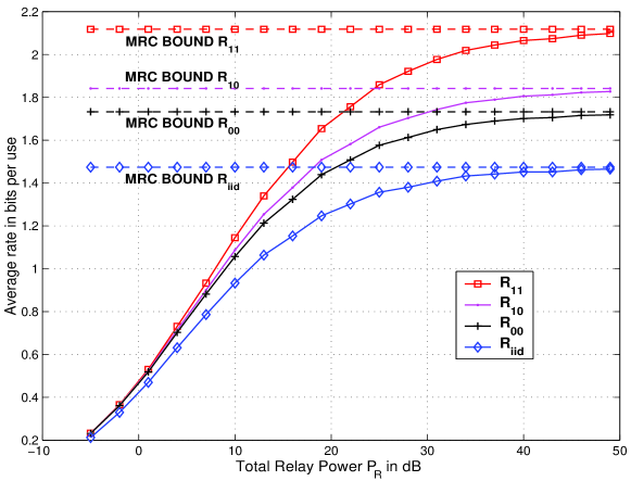
Figure 5: Average rate of a single user system as a function of total relay power $P_{R}$ for $P=P_{I}=10$.

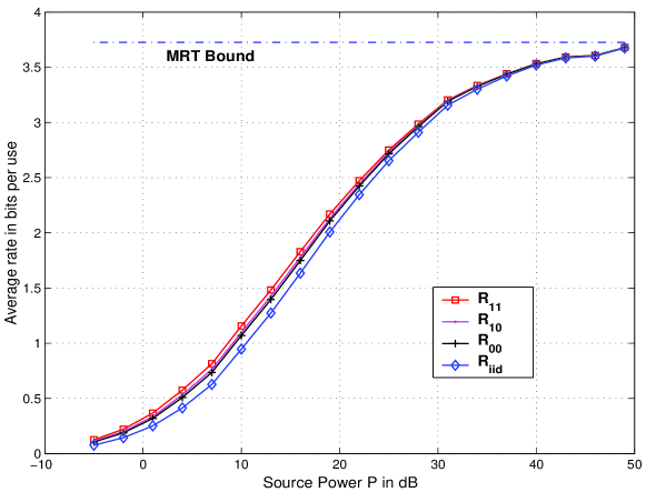
Figure 6: Average rate of a single user system as a function of source power $P$ for $P_{R}=P_{I}=10$.

We consider a common-interference based model to generate the relay noise covariance matrix. Each relay in addition to its thermal noise observes faded versions of common interference signals. The effective relay noise including both the interference and the local noise is given by

$${\bf n_{eff}}=\sum_{k=1}^{Q}{\bf h_{k}}i_{k}+{\bf n_{R}}$$ (38)

where $i_{k}$ is the signal transmitted by the $k^{th}$ interferer and ${\bf h_{k}}$ is the channel between the relays and the $k^{th}$ interferer. The covariance matrix is given by

$${\bf K}=\mathbb{E}[{\bf n_{eff}n_{eff}^{\dagger}}]=\sum_{k=1}^{Q}{\bf h_{k}h_{k}^{\dagger}}P_{I_{k}}+{\bf I}.$$ (39)

The total interference power is $P_{I}=\sum_{k=1}^{Q}P_{I_{k}}$. Fig. 5 plots the average rate per channel-use as a function of the total relay power for $P=P_{I}=10$ for the case of two relays and one interferer. The main observations are

1. The performance order of the schemes in (35) which was obtained at high $P_{R}$ is valid at all values of $P_{R}$.

2. The difference ($R_{11}-R_{10}$) which indicates the benefits of learning correlation increases with relay power. With increase in relay power, the schemes diverge in performance, which is an indication that correlation impacts more at high relay power.

In Fig. 6, we plot the average rate as a function of source transmit power for $P_{R}=P_{I}=10$. Clearly, with increase in source power, the schemes achieve the MRT bound. Therefore the effect of correlation is less pronounced with increasing source power. Fig. 7 shows the average rate as a function of the interference power for one interfering node and two relays. As one can expect, the average rate decreases with $P_{I}$. However $R_{11}$ does not reach zero even at infinite interference power. This can be explained through the following: With one interfering source and $N$ relays, the average SNR for Scheme-11 at very high $P_{R}$ is given by

$$\mathbb{E}[\mbox{SNR}_{11}]=(N-1)+\mathbb{E}\left[\frac{1}{1+P_{I}\parallel{\bf h_{1}}\parallel^{2}}\right].$$ (40)

This suggests that the average SNR is at least $N-1$ irrespective of the interference power. However, the average SNR decreases when the number of interfering sources increases. This is due to loss in degrees of freedom due to increase in the range space of interference.

Fig. 8 shows the average sum rate versus the number of relays. The covariance matrix is generated with the help of 9 interferers with total power $P_{I}=200$. It can be noticed that the sum rate increases at a greater rate when the number of relays is greater than the number of interferers. As $P_{I}\rightarrow\infty$, $R_{11}\rightarrow 0$ when the number of relays is less than the number of interferers ($N\leq Q$). However for ($N>Q$), $R_{11}$ does not vanish even when $P_{I}\rightarrow\infty$.

Remark

As we discussed earlier, the relay design problem is a tradeoff between canceling the interference and maximizing the signal power. At very high interference power, it is important to cancel the interference. At high $P_{R}$ since the network behaves as a SIMO system with $N$ antennas at the receiver, up to $(N-1)$ interfering sources can be rejected. When the number of interferers is more than the total number of relays, interference cannot be completely nulled.

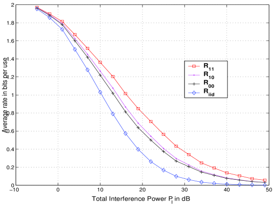
Figure 7: Average rate of a single user system as a function of interference power $P_{I}$ for $P=10$ and $P_{R}=100$.

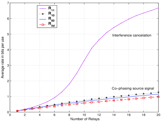
Figure 8: Average rate of a single user system as a function of the number of relays with 9 interferers of total power $P_{I}=200$ (23 dB), and $P=10$.

III-D Impact of channel knowledge at the relays

Throughout this paper, we assume that the relays have perfect knowledge of all the channels in the network. It may seem that complete channel knowledge is required at the relays for the relationship in (35) to hold. In Scheme-11, since the relays know the noise covariance matrix, they must also know the channels between the relays and interferers (when the number of interferers is less than the number of relays). This information is not available at the relays for Scheme-10. Still, it performs better than Scheme-00 where there is no noise correlation. In fact, it can be shown that Scheme-10 outperforms Scheme-00 even when there is absolutely no channel knowledge at the relays including the source-relay and relay-destination channels. This is also true when the relays only have local channel information. That is, relay $R_{i}$ knows only its forward and backward channels ${\bf f}(i)$ and ${\bf g}(i)$. The following theorem states these results:

Theorem 4

The average achievable rate for a relay network is lesser with relay noise covariance matrix $\bf K\odot I$ than with any general $\bf K$, where only local channel knowledge is available at the relays. In other words

$$\mathbb{E}[\log(1+\mbox{SNR}_{10})]\geq\mathbb{E}[\log(1+\mbox{SNR}_{00})].$$ (41)

Further, when there is absolutely no CSI available at the relays, Scheme-10 outperforms Scheme-00 in terms of the average SNR, i.e. $\mathbb{E}[\mbox{SNR}_{10}]\geq\mathbb{E}[\mbox{SNR}_{00}]$.

Proof:

Refer to the Appendix. ∎

It is now clear that relay noise correlation is always helpful regardless of the channel and correlation knowledge at the relays. For maximizing signal power channel knowledge is essential while correlation knowledge is required to minimize interference power. With perfect channel knowledge, increasing the number of relays (while keeping the total relay power fixed) is helpful as signal power is increased due to coherent combining.

IV Three-hop parallel relay network

Figure 9: Three-hop parallel relay network

In this section, we consider another application of the relay network with correlated noise. Consider a three-hop relay network as shown in Fig. 9. This is an example of a multi-stage relay network. There are $N$ and $M$ relays in the first and second stages respectively. Let the power expended by the source, the first stage relays, the second stage relays be $P_{0}$, $P_{1}$ and $P_{2}$ respectively. We denote this network with the shorthand notation $\mathfrak{R}_{3}(P_{0},{\bf f},{\bf d_{1}},P_{1},{\bf H},{\bf d_{2}},P_{2},{\bf g})$. In the first slot, the received signal at the first stage relays is given by

$${\bf r_{1}=f}x+{\bf n_{1}}.$$ (42)

The relay transmitted signal is given by $\bf{t_{r_{1}}=D_{1}r_{1}}$, where $\bf D_{1}$ satisfies the power constraint of the first stage relays, i.e. $\mbox{Tr}({\bf{D_{1}D_{1}^{\dagger}}({\bf ff^{\dagger}}P+{\bf I})})=P_{1}$. Here $\bf D_{1}=\mbox{diag}(d_{1})$. In the second time slot, the relays at the second stage receive

$$\bf{r_{2}=HD_{1}r_{1}+n_{2}}=\bf{HD_{1}f}x+{\bf HD_{1}n_{1}+n_{2}}.$$ (43)

In the third slot, the signal transmitted by the second stage relays is $\bf t_{r_{2}}=D_{2}r_{2}$. The power constraint at the second stage relays is given by $\mathbb{E}\left[\parallel\bf t_{r_{2}}\parallel^{2}\right]=P_{2}$, which results in

$$\mbox{Tr}\left({\bf D_{2}D_{2}^{\dagger}}({\bf HD_{1}ff^{\dagger}D_{1}^{\dagger}H^{\dagger}}P_{0}+{\bf HD_{1}D_{1}^{\dagger}H^{\dagger}+I})\right)=P_{2}.$$ (44)

Notice that the choice of $\bf D_{1}$ affects the power constraint at $\bf D_{2}$. The received signal at the destination is given by

$$y={\bf g^{T}t_{r_{2}}} = {\bf g^{T}D_{2}}\left({\bf HD_{1}}({\bf f}x+{\bf n_{1}})+{\bf n_{2}}\right)+n$$ (45)

$$= {\bf g^{T}D_{2}HD_{1}f}x+{\bf g^{T}D_{2}HD_{1}n_{1}}+{\bf g^{T}D_{2}n_{2}}+n.$$ (46)

Note that both the relay stages operate at their maximum power. For any feasible $\bf D_{2}$ and $\bf D_{1}$, the SNR is defined as

$$\mbox{SNR}({\bf D_{1}},{\bf D_{2}})=\frac{\left|{\bf g^{T}D_{2}HD_{1}f}\right|^{2}P_{0}}{{\parallel\bf g^{T}D_{2}HD_{1}\parallel^{2}}+\parallel{\bf g^{T}D_{2}}\parallel^{2}+1}.$$ (47)

The relay design problem is stated below as

$$\max_{{\bf D1,D_{2}}}\mbox{SNR}({\bf D_{1},D_{2}}),$$ (48)

$$\mbox{s.t.}~{}~{}~{}\mbox{Tr}({\bf{D_{1}D_{1}^{\dagger}}({\bf ff^{\dagger}}P+{\bf I})})=P_{1},$$ (49)

$$\mbox{and}~{}~{}~{}~{}\mbox{Tr}\left({\bf D_{2}D_{2}^{\dagger}}({\bf HD_{1}ff^{\dagger}D_{1}^{\dagger}H_{2}^{\dagger}}P_{0}+{\bf HD_{1}D_{1}^{\dagger}H^{\dagger}+I})\right)=P_{2}.$$ (50)

To solve this problem directly can be difficult as the constraints are interdependent. We therefore approach the problem differently. Now consider any feasible $\bf D_{1}$ for the first stage relays. Once the relay operation for the first stage relays is fixed, the network reduces to a two hop parallel relay network with correlated noise $\mathfrak{R}_{2}(P_{0},{\bf f_{\mbox{new}}},{\bf D_{2}},P_{2},{\bf g})$ where

$${\bf f_{\mbox{new}}=HD_{1}f}.$$ (51)

By comparing (46) and (2), relay noise in the reduced two hop network can be found as

$${\bf n_{R}=HD_{1}n_{1}+n_{2}}.$$ (52)

Note that the noise in (52) is correlated and the corresponding covariance matrix is given by

$${\bf K=HD_{1}D_{1}^{\dagger}H^{\dagger}+I}.$$ (53)

Now that the network is a dual-hop parallel relay network, we can utilize the result in Theorem 1 to solve the relay optimization for the second stage relays. We have from (7)

$${\bf d_{2}^{\circ}}({\bf D_{1}}) = \kappa\left(\left[{\bf GKG^{\dagger}}P_{2}+({\bf f_{\mbox{new}}f_{\mbox{new}}^{\dagger}\odot I})P_{0}+{\bf K\odot I}\right]^{-1}({\bf f_{\mbox{new}}\odot g})\right)^{*}.$$ (54)

We therefore are able to determine the optimal design for the second stage relays for all feasible relay gain vectors for the first stage. Similarly if we can find optimal $\bf D_{1}$ for all possible $\bf D_{2}$ we can then resort to iterating between the solutions. However the problem is that the second stage relays’ power constraint is affected by $\bf D_{1}$. Therefore fixing $\bf D_{2}$ and finding the optimal $\bf D_{1}$ can violate the power constraint for the second stage. One way to solve this problem is to use the reciprocity property of AF relay networks recently proved in [2]. We state the theorem from [2] in the following.

Theorem 5

[2] The capacity of a three-hop relay network is unchanged when the role of the transmitter and the receiver is switched while maintaining the same transmit power at each hop for both the original and reciprocal channels. This is equivalent to

$$\mathfrak{R}_{3}(P_{0},{\bf f},{\bf d_{1}},P_{1},{\bf H},{\bf d_{2}},P_{2},{\bf g})=\mathfrak{R}_{3}(P_{2},{\bf g},\kappa_{2}{\bf d_{2}},P_{1},{\bf H^{T}},\kappa_{1}{\bf d_{1}},P_{0},{\bf f}),$$ (55)

where the constants $\kappa_{1}$ and $\kappa_{2}$ ensures power constraint compliance in the reciprocal network. (Note that we allow some abuse of notation as the above statement implies that the capacity of the two networks are the same.)

Using the above result, one can reverse the direction of the communication in the relay network. For the reciprocal network, the gain of the first stage relays is related to the gain of the second stage relays through a constant multiplying factor which can be obtained from the power constraint as follows:

$$\kappa_{2}^{2}=\frac{P_{1}}{\mbox{Tr}\left({\bf D_{2}D_{2}^{\dagger}}({\bf gg^{\dagger}}P_{2}+{\bf I})\right)}$$ (56)

Similarly $\kappa_{1}$ is found as

$$\kappa_{1}^{2}=\frac{P_{0}}{\mbox{Tr}\left({\bf D_{1}D_{1}^{\dagger}}(\kappa_{2}^{2}{\bf H^{T}D_{2}gg^{\dagger}D_{2}^{\dagger}H^{*}}P_{2}+\kappa_{2}^{2}{\bf H^{T}D_{2}D_{2}^{\dagger}H^{*}+I})\right)}.$$ (57)

As discussed earlier, the reciprocal network can be reduced to a two hop network and the relay gain for the second stage can be optimized. Using Theorem 1, we can find the optimal gain for the second stage of the reciprocal network (which is proportional to the first stage relay of the original network) for every feasible $\kappa_{2}{\bf D_{2}}$. The procedure then will be to find the optimal relay gain for the second stage having the first stage gain fixed. The next step is to find the reciprocal network and optimize the second stage, and iterate this procedure till convergence is achieved. The algorithm is listed in Table I.

TABLE I: Algorithm: three-hop Relay Network Optimization

1. Choose any ${\bf D_{1}}$ that satisfies the first stage power constraint.

2. Reduce the network to a two hop network with noise correlation.

3. Find the optimal ${\bf D_{2}^{\circ}(D_{1})}$.

4. Begin Loop:

5. Determine the reciprocal network.

6. Optimize the second stage relays.

7. Repeat until convergence.

8. End Loop

Remark

Notice that the capacity of the network increases with every iteration as each iteration involves optimization. This suggests that the algorithm will eventually converge. Although it is not known if the algorithm guarantees a global optimum solution, based on extensive numerical simulations, we conjecture that the algorithm outputs the global optima whenever there is convergence.

Figure 10: Pictorial representation of the relay optimization algorithm.

Fig. 11 shows the convergence of the algorithm for a variety of initial relay amplification factors. In the simulation, the channel matrices are

$${\bf f}=[1~{}6],~{}{\bf g}=[4~{}-3],~{}{\bf H}=[2~{}-3;4~{}2].$$

We use the following initial inputs for the first stage relay gains every time the algorithm begins:

$${\bf d_{1}}(1)=[1~{}0],~{}{\bf d_{1}}(2)=[0~{}1],~{}{\bf d_{1}}(3)=[-2~{}1],~{}{\bf d_{1}}(4)=[2~{}1],~{}{\bf d_{1}}(5)=[-20,~{}-1].$$

The transmit power at each hop is unity ($P_{0}=P_{1}=P_{2}=1$). At the start of the algorithm, the inputs will be scaled to satisfy the power constraint. For each input, the progress of the algorithm (measured in terms of SNR at the destination) is displayed in Fig. 11. For all these inputs, the algorithm converges to an SNR value of 6.5638 while the first and second stage relay gains converge to

$${\bf\hat{d_{1}}}=[-0.0823~{}-0.1633],~{}{\bf\hat{d_{2}}}=[0.2533~{}0.2566].$$

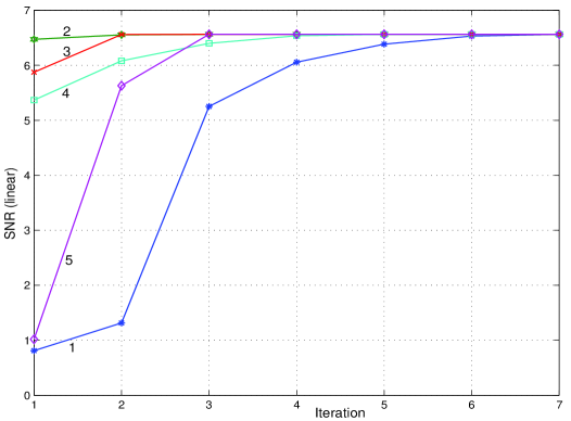
Figure 11: Convergence of the algorithm for different initial inputs (${\bf d_{1}}$).

In the following we study the characteristics of three-hop relay networks in the high-power regimes. The proofs are available in the Appendix.

IV-A Properties of $\mathfrak{R}_{3}(P_{0},{\bf f},{\bf d_{1}},P_{1},{\bf H},{\bf d_{2}},P_{2},{\bf g})$

1. $P_{2}\rightarrow\infty$:  When there is no power constraint (or infinite power) for the last stage relays, the three-hop network for the optimal $\bf D_{2}$ reduces to a two hop network with the destination consisting of multiple antennas. This is equivalent to

   $$\mathfrak{R}_{3}(P_{0},{\bf f},{\bf d_{1}},P_{1},{\bf H},{\bf d_{2}=d_{2}^{\circ}},P_{2}=\infty,{\bf g})=\mathfrak{R}_{2}(P_{0},{\bf f},{\bf d_{1}},P_{1},{\bf H}).$$ (58)

   It is worth noting that the noise at the multiple antenna destination of the reduced network is correlated.

2. $P_{0}\rightarrow\infty$:  For the case where the source power is infinite, it is clear from the properties in Section II-C that the noise terms at the first stage relays are negligible. This reduces the network to a two-hop relay network with a multiple antenna source.

   $$\mathfrak{R}_{3}(P_{0}=\infty,{\bf f},{\bf d_{1}=d_{1}^{\circ}},P_{1},{\bf H},{\bf d_{2}},P_{2},{\bf g})=\mathfrak{R}_{2}(P_{1},{\bf H},{\bf d_{2}},P_{2},{\bf g})$$

   The network optimization for the reduced network involves joint precoder (transmit covariance matrix) and relay design which are interdependent. We can utilize the algorithm in Table I for this optimization.

3. $P_{0},P_{2}\rightarrow\infty$:  When the power of both the source and the last stage relays tend to $\infty$, the relay network reduces to a point to point MIMO channel with the constraint that the rank of the input covariance matrix is one.

   $$\mathfrak{R}_{3}(P_{0}=\infty,{\bf f},{\bf d_{1}=d_{1}^{\circ}},P_{1},{\bf H},{\bf d_{2}=d_{2}^{\circ}},P_{2},{\bf g})=\mathfrak{R}_{1}(P_{1},{\bf H})$$

   Here $\mathfrak{R}_{1}(P_{1},{\bf H})$ indicates that the network is a single-hop point to point channel. Thus the three-hop network optimization problem is equivalent to SNR maximization problem in the point to point MIMO channel. The optimal strategy is beamforming along the principal eigen-vector of the channel matrix.

4. $P_{1},P_{2}\rightarrow\infty$:  For this scenario the last two stages can be removed and the network reduces to a point to point SIMO channel with receive combining vector $\bf g^{T}D_{2}HD_{1}$. Optimizing one set of relays is enough to achieve the point to point channel capacity.

   $$\mathfrak{R}_{3}(P_{0},{\bf f},{\bf d_{1}},P_{1},{\bf H},{\bf d_{2}=d_{2}^{\circ}},P_{2}=\infty,{\bf g})=\mathfrak{R}_{1}(P_{0},{\bf f}).$$

   $\mathfrak{R}_{1}(P_{0},{\bf f})$ indicates that the network is a single-hop point to point channel.

5. $P_{0},P_{1}\rightarrow\infty$:  When the source and the first stage relays have very high power, the network reduces to a point to point MISO system with transmit precoding vector $\bf D_{2}HD_{1}f$. Like the previous case, optimizing one set of relays suffices to optimize the whole network.

   $$\mathfrak{R}_{3}(P_{0}=\infty,{\bf f},{\bf d_{1}},P_{1}=\infty,{\bf H},{\bf d_{2}=d_{2}^{\circ}},P_{2},{\bf g})=\mathfrak{R}_{1}(P_{2},{\bf g})$$

Remark

In all the above cases, if the transmit power at any hop is very high, noise at the receive side is negligible. When this occurs at the first or the last hop, (for example, $P_{0}$ or $P_{2}\rightarrow\infty$) the hop can be removed. Here any rate that can be achieved in the original network is achievable in the reduced network and vice versa. For example consider the three-hop case where the source has one antenna, and 5 relays in the first stage. When the source power is very high ($P_{0}\rightarrow\infty$) then the first hop network can be removed, and the reduced network consists of two hops. In the new network the source consists of 5 antennas and transmits a one dimensional signal. It is interesting that the two networks are equivalent.

V Conclusion

In this work, we considered an AF relay network wherein the relay noises are correlated which may be due to common interference or multi-hop AF relaying. We obtained closed form expressions for optimal rate maximizing relay gains and maximum achievable rate when correlation knowledge is available at the relays for both single-user and multi-source scenarios. Further we showed that correlation does not hurt irrespective of channel and correlation knowledge at the relays. We also showed that correlation knowledge results in significant performance improvement. Analytical and simulation results demonstrate significant rate enhancement when correlation knowledge is exploited. With appropriate gains, the relays can perform distributed interference cancelation when the number of relays is greater than the the number of interferers. The performance improvement increases with the total relay power and the number of relays. As there are significant benefits in learning correlation, practical schemes to communicate the correlation structure to the relays need to be explored.

For three-hop AF relay networks, we addressed the relay optimization problem. By fixing relay gains for one of the stages we reduced the network to a two hop network with noise correlation. Combining the result we obtained for two hop networks with correlated noise and a multi-hop duality result from [2], we propose an iterative algorithm that increases capacity for every iteration. This algorithm can be utilized for joint optimization of relay gains and precoder in multi-antenna sources.

-A Proof of Theorem 1

From the destination received signal in (2), the achievable rate is given by $R=\log_{2}(1+\mbox{SNR})$ where

$$\mbox{SNR}=\frac{{\bf d^{T}G}{\bf ff^{\dagger}}{\bf G^{\dagger}d^{*}}P}{{\bf d^{T}GKG^{\dagger}d^{*}}+1}.$$ (59)

It is worth noting that ${\bf d}$ should satisfy the sum power constraint of the relays.

$${\bf d^{T}}\left[\left({\bf ff^{\dagger}}P+{\bf K}\right)\odot{\bf I}\right]{\bf d^{*}}=P_{R}$$ (60)

Now we are interested in maximizing the sum rate over all possible relay amplification vectors that satisfy the relay power constraint. The above problem is equivalent to maximizing SNR with respect to ${\bf d}$.

$$\mbox{SNR}^{\circ}=\max_{\bf d}\mbox{SNR}$$

Incorporating (60) into the denominator of (59), we have

SNR $$= \frac{{\bf d^{T}G}{\bf ff^{\dagger}}{\bf G^{\dagger}d^{*}}PP_{R}}{{\bf d^{T}GKG^{\dagger}d^{*}}P_{R}+{\bf d^{T}}\left[\left({\bf ff^{\dagger}}P+{\bf K}\right)\odot{\bf I}\right]{\bf d^{*}}}$$

$$= \frac{{\bf d^{T}G}{\bf ff^{\dagger}}{\bf G^{\dagger}d^{*}}PP_{R}}{{\bf d^{T}}\left[{\bf GKG^{\dagger}}P_{R}+\left({\bf ff^{\dagger}}P+{\bf K}\right)\odot{\bf I}\right]{\bf d^{*}}}$$ (61)

Define the matrices A and B:

$${\bf A}=\left[{\bf GKG^{\dagger}}P_{R}+\left({\bf ff^{\dagger}}P+{\bf K}\right)\odot{\bf I}\right]$$ (62)

$${\bf B}={\bf G}{\bf ff^{\dagger}}{\bf G^{\dagger}}PP_{R}$$ (63)

Notice that the matrix ${\bf A}$ is Hermitian and positive definite while $\bf B$ is Hermitian and positive semi-definite. By Cholesky decomposition ${\bf A=LL^{\dagger}}$, we have

$$\mbox{SNR}=\frac{{\bf d^{T}Bd^{*}}}{{\bf d^{T}LL^{\dagger}d^{*}}}$$ (64)

Let ${\bf w^{T}=d^{T}L}$, we have

$$\mbox{SNR}=\frac{{\bf w^{T}L^{-1}BL^{-\dagger}w^{*}}}{{\bf w^{T}w^{*}}}$$ (65)

The relay optimization problem is therefore

$$\mbox{SNR}^{\circ}=\max_{{\bf w}}\frac{{\bf w^{T}L^{-1}BL^{-\dagger}w^{*}}}{{\bf w^{T}w^{*}}}$$ (66)

By utilizing Rayleigh Quotient we have

$$\mbox{SNR}^{\circ}=\lambda_{\max}({\bf L^{-1}BL^{-\dagger}})$$ (67)

$${\bf w}^{\circ}=\left({\bf v}_{\max}({\bf L^{-1}BL^{-\dagger}})\right)^{*}$$ (68)

where $\lambda_{\max}({\bf P})$ and $v_{\max}({\bf P})$ are the principal eigen-value and eigen-vector of the matrix ${\bf P}$.
Since ${\bf B=(f\odot g)(f\odot g)^{\dagger}}PP_{R}$, we have

$$\mbox{SNR}^{\circ} = PP_{R}\lambda_{\max}({\bf L^{-1}(f\odot g)(f\odot g)^{\dagger}L^{-\dagger}})$$ (69)

$$= PP_{R}\lambda_{\max}({\bf(f\odot g)^{\dagger}L^{-\dagger}L^{-1}(f\odot g)})$$ (70)

$$= PP_{R}\lambda_{\max}({\bf(f\odot g)^{\dagger}A^{-1}(f\odot g)})$$ (71)

$$= PP_{R}{\bf(f\odot g)^{\dagger}A^{-1}(f\odot g)}$$ (72)

where (70) follows from the property that the non-zero eigen values of $\bf AB$ are equal to those of $\bf BA$. (71) holds since $\bf L^{-\dagger}L^{-1}=(LL^{\dagger})^{-1}=A^{-1}$. The optimal relay amplification vector is given by

$${\bf d}^{\circ} = \kappa\left({\bf L^{-\dagger}}{\bf v}_{\max}({\bf L^{-1}BL^{-\dagger}})\right)^{*}$$ (73)

$$= \kappa\left({\bf L^{-\dagger}}{\bf L^{-1}}({\bf f\odot g})\right)^{*}$$ (74)

$$= \kappa\left({\bf A^{-1}(f\odot g)}\right)^{*}.$$ (75)

where $\kappa$ ensures compliance with the relay power constraint. Hence proved. ∎

-B Proof of Properties in Section II-C

1. $P_{R}\rightarrow\infty$: At high relay power $P_{R}$, for any relay amplification vector $\bf d$, the destination noise is negligible. In that case, the input-output relationship can be expressed as

   $$y={\bf(d\odot g)^{T}f}x+{\bf(d\odot g)^{T}n_{R}},$$

   which is equivalent to a SIMO system, ${\bf y=f}x+{\bf n_{R}}$ , with the receive combining vector $\bf d\odot g$. Now consider the maximum achievable SNR (corresponding to $\bf d^{\circ}$) from (6), which is

   $$\mbox{SNR}^{\circ}=PP_{R}({\bf f\odot g})^{\dagger}{\bf A^{-1}}({\bf f\odot g}).$$

   At high $P_{R}$, ${\bf A=(GKG^{\dagger})}P_{R}$ which leads to

   $$\mbox{SNR}^{\circ}=P({\bf f\odot g})^{\dagger}{\bf(GKG^{\dagger})^{-1}}({\bf f\odot g})=P{\bf f^{\dagger}K^{-1}f}.$$

   At high $P_{R}$, the optimal relay functionality becomes

   $${\bf d^{\circ}}=\kappa{\bf(GKG^{\dagger})^{-1}}({\bf f\odot g})=\kappa{\bf G^{-\dagger}K^{-1}G^{-1}Gf}=\kappa{\bf G^{-\dagger}K^{-1}f}.$$

   Thus ${\bf d=\kappa G^{-\dagger}K^{-1}f}$ achieves the MRC bound when $P_{R}\rightarrow\infty$.

2. $P\rightarrow\infty$:  When the source power is high, it can be observed that the relay noise terms are negligible. The input-output relationship is then given by

   $$y={\bf g^{T}\frac{(d\odot f)}{\sqrt{(d\odot f)^{\dagger}(d\odot f)}}}\sqrt{{\bf(d\odot f)^{\dagger}(d\odot f)}}x+n.$$

   which represents a MISO system with the beamforming vector $\bf\frac{(d\odot f)}{\sqrt{(d\odot f)^{\dagger}(d\odot f)}}$. Since ${\bf(d\odot f)^{\dagger}(d\odot f)}P=P_{R}$, the input transmit power is $P_{R}$. For the optimal relay design $\bf d^{\circ}$ we have ${\bf A=(ff^{\dagger}\odot I)}P$, which results in

   $$\mbox{SNR}^{\circ}=P_{R}({\bf f\odot g})^{\dagger}{\bf(ff^{\dagger}\odot I)^{-1}}({\bf f\odot g})=P_{R}{\bf g^{\dagger}g}.$$

   The system thus behaves as a multiple antenna transmitter with a single antenna receiver. ∎

-C Proof of Theorem 2

From the destination received signal in (13), we can notice that due to relay amplification, the relay network is equivalent to a scalar MAC. The sum rate is given by

$$R=\log(1+\mbox{SNR})$$

where

$$\mbox{SNR}=\frac{{\bf d^{T}G}\left(\sum_{k=1}^{L}{\bf f_{k}f_{k}^{\dagger}}P_{k}\right){\bf G^{\dagger}d^{*}}}{{\bf d^{T}GKGd^{*}}+1}.$$ (76)

Notice that ${\bf d}$ satisfies the sum power constraint of the relays.

$${\bf d^{T}}\left[\left(\sum_{k=1}^{L}{\bf f_{k}f_{k}^{\dagger}}P_{k}+{\bf K}\right)\odot{\bf I}\right]{\bf d^{*}}=P_{R}$$ (77)

Now we are interested in maximizing the sum rate over all possible relay amplification vectors that satisfy the relay power constraint. The above problem is equivalent to maximizing SNR with respect to ${\bf d}$.

$$\mbox{SNR}^{\circ}=\max_{\bf d}\mbox{SNR}$$

Incorporating (77) into the denominator of (76), we have

SNR $$= \frac{{\bf d^{T}G}\left(\sum_{k=1}^{L}{\bf f_{k}f_{k}^{\dagger}}P_{k}\right){\bf G^{\dagger}d^{*}}P_{R}}{{\bf d^{T}GKG^{\dagger}d^{*}}P_{R}+{\bf d^{T}}\left[\left(\sum_{k=1}^{L}{\bf f_{k}f_{k}^{\dagger}}P_{k}+{\bf K}\right)\odot{\bf I}\right]{\bf d^{*}}}$$

$$= \frac{{\bf d^{T}G}\left(\sum_{k=1}^{L}{\bf f_{k}f_{k}^{\dagger}}P_{k}\right){\bf G^{\dagger}d^{*}}P_{R}}{{\bf d^{T}}\left[{\bf GKG^{\dagger}}P_{R}+\left(\sum_{k=1}^{L}{\bf f_{k}f_{k}^{\dagger}}P_{k}+{\bf K}\right)\odot{\bf I}\right]{\bf d^{*}}}$$ (78)

Define the matrices A and B:

$${\bf A}=\left[{\bf GKG^{\dagger}}P_{R}+\left(\sum_{k=1}^{L}{\bf f_{k}f_{k}^{\dagger}}P_{k}+{\bf K}\right)\odot{\bf I}\right]$$ (79)

$${\bf B}={\bf G}\left(\sum_{k=1}^{L}{\bf f_{k}f_{k}^{\dagger}}P_{k}\right){\bf G^{\dagger}}P_{R}$$ (80)

Then, proceeding as in the proof for Theorem 1, we have.

$$\mbox{SNR}^{\circ} = \lambda_{\max}({\bf A^{-1}B})$$ (81)

and the optimal relay amplification vector is given by

$${\bf d}^{\circ}=\left({\bf v}_{\max}({\bf A^{-1}B})\right)^{*}.$$ (82)

Hence proved. ∎

-D Proof of Theorem 3

From (28) and (29) we have

$$\mbox{SNR}_{00}=a~{}~{}~{}~{}~{}~{}~{}~{}\mbox{SNR}_{10}=\frac{a^{2}}{a+b}$$ (83)

where

$$a=\sum_{i=1}^{N}\frac{|{\bf f}(i)|^{2}}{{\bf K}_{ii}}.$$ (84)

$$b=\sum_{i=1}^{N}\sum_{j=1~{}j\neq i}^{N}\frac{{\bf f}(i){\bf f^{*}}(j){\bf K}_{ij}}{{\bf K}_{ii}{\bf K}_{jj}}$$ (85)

Now consider the the difference in SNR of Scheme-10 and Scheme-00, which is given by

$$\mbox{SNR}_{10}-\mbox{SNR}_{00}=\frac{-ab}{a+b}$$ (86)

Notice that the difference $\mbox{SNR}_{10}-\mbox{SNR}_{00}$ is convex in the correlation term $b$ as its second derivative w.r.t. $b$ is non-negative. We assume that the magnitude and phase of the components of ${\bf f}$ are independent where the magnitude follows Rayleigh distribution while the phase is uniformly distributed in the interval $[0,2\pi]$. Conditioned on the magnitude of the channels, the average of $b$ over all channel phases is 0. By applying Jensen’s inequality we have

$$\mathbb{E}[\mbox{SNR}_{10}-\mbox{SNR}_{00}]\geq 0.$$

Let us now consider the difference in rate $R_{10}-R_{00}$.

$$R_{10}-R_{00}=\mathbb{E}\left[\log\left(\frac{1+\mbox{SNR}_{10}}{1+\mbox{SNR}_{00}}\right)\right]=\log\left(\frac{1+\frac{a^{2}}{a+b}}{1+a}\right).$$ (87)

It can be shown that the difference $R_{10}-R_{00}$ is convex in $b$. Therefore through Jensen’s inequality

$$\mathbb{E}[R_{10}-R_{00}]\geq 0.$$ (88)

Hence proved. ∎

-E Proof of Theorem 4

For any constant relay gain $\bf D$ for the relays, the SNR of the two schemes where the relay noise covariance matrix is $\bf K$ and $\bf K\odot I$ respectively are

$$\mbox{SNR}_{10}=\frac{{\bf\left|g^{T}Df\right|^{2}}P}{{\bf g^{T}DKD^{*}g^{*}}+1}$$

$$\mbox{SNR}_{00}=\frac{{\bf\left|g^{T}Df\right|^{2}}P}{{\bf g^{T}D(K\odot I)D^{*}g^{*}}+1}$$

Note that the power expended by the relays is the same in both the schemes. When the relays have only local channel knowledge, the phase of the relays should be such that the phase of the forward and backward channels are canceled. We therefore have

$$\mbox{SNR}_{10}=\frac{c}{b+a}~{}\mbox{and}~{}\mbox{SNR}_{00}=\frac{c}{b}$$

where

$$a=\sum_{i=1}^{N}\sum_{j=1~{}j\neq i}^{N}{\bf g}(i){\bf g^{*}}(j){\bf d}(i){\bf d}^{*}(j){\bf K}_{ij}$$

$$b=\sum_{i=1}^{N}|{\bf g}(i)|^{2}|{\bf d}(i)|^{2}{\bf K}_{ii}$$

$$c=\left(\sum_{i=1}^{N}|{\bf d}(i){\bf g}(i){\bf f}(i)|\right)^{2}.$$

The term $a$ depends on both magnitude and phase of the channels while $b$ and $c$ depend only on the magnitude of the channels. It can be shown that $\log(1+\mbox{SNR}_{10})$ is convex in $a$. Given the magnitude of the channels, the average of $a$ over channel phases is zero. Therefore by Jensen’s inequality

$$\mathbb{E}_{a,b,c}\left[\log(1+\mbox{SNR}_{10})\right]\geq\mathbb{E}_{b,c}\left[\log\left(1+\frac{c}{b}\right)\right]=\mathbb{E}_{b,c}\left[\log(1+\mbox{SNR}_{00})\right].$$

Now consider the case where the relays have no CSI. Here the relay gain $\bf D$ is independent of $\bf f$ and $\bf g$. Taking expectation of $\mbox{SNR}_{10}$ and $\mbox{SNR}_{00}$ over $\bf f$, we have

$$\mathbb{E}_{{\bf f}}[\mbox{SNR}_{10}]=\frac{{\bf\parallel g^{T}D\parallel^{2}}P}{{\bf g^{T}DKD^{*}g^{*}}+1}$$ (89)

$$\mathbb{E}_{{\bf f}}[\mbox{SNR}_{00}]=\frac{{\bf\parallel g^{T}D\parallel^{2}}P}{{\bf g^{T}D(K\odot I)D^{*}g^{*}}+1}$$ (90)

where $\mathbb{E}[{\bf ff^{\dagger}}]={\bf I}$. Observe that (89) is dependent on the phase of $\bf g$ while (90) is independent of phase of $\bf g$. From Jensen’s inequality it can be easily seen that $\mathbb{E}[\mathbb{E}_{\bf f}[\mbox{SNR}_{10}]]\geq\mathbb{E}[\mathbb{E}_{\bf f}[\mbox{SNR}_{00}]]$. Hence proved. ∎

-F Proof of Properties in Section IV-A

From (46), the received signal at the destination for the three-hop case is given by

$$y={\bf g^{T}D_{2}HD_{1}f}x+{\bf g^{T}D_{2}HD_{1}n_{1}}+{\bf g^{T}D_{2}n_{2}}+n.$$ (91)

Let ${\bf D_{1}}=\sqrt{P_{1}}{\bf D_{1}^{u}}$ and ${\bf D_{2}}=\sqrt{P_{2}}{\bf D_{2}^{u}}$ where ${\bf D_{i}^{u}}$ expends unit power at the $i^{th}$ stage relays, $i\in\{1,2\}$. Similarly let $x=\sqrt{P_{0}}x^{\prime}$ where $\mathbb{E}[|x^{\prime}|^{2}]=1$. Now the effective received signal at the destination is

$$y^{\prime}={\bf g^{T}D_{2}^{u}HD_{1}^{u}f}x^{\prime}+\frac{{\bf g^{T}D_{2}^{u}HD_{1}^{u}n_{1}}}{\sqrt{P_{0}}}+\frac{\bf g^{T}D_{2}^{u}n_{2}}{\sqrt{P_{1}}}+\frac{n}{\sqrt{P_{2}}}.$$ (92)

The modified power constraints are

$$\mbox{Tr}\left({\bf{D_{1}^{u}D_{1}^{u\dagger}}}\left({\bf ff^{\dagger}}+\frac{{\bf I}}{P_{0}}\right)\right)=1,$$ (93)

$$\mbox{Tr}\left({\bf D_{2}^{u}D_{2}^{u\dagger}}\left({\bf HD_{1}^{u}ff^{\dagger}D_{1}^{u}H_{2}^{\dagger}}+\frac{\bf HD_{1}D_{1}^{\dagger}H^{\dagger}}{P_{0}}+\frac{\bf I}{P_{1}}\right)\right)=1.$$ (94)

1. $P_{2}\rightarrow\infty$:
   At very high $P_{2}$, the normalized input-output relation becomes

   $$y^{\prime} = {\bf g^{T}D_{2}^{u}HD_{1}f}x^{\prime}+\frac{{\bf g^{T}D_{2}^{u}HD_{1}^{u}n_{1}}}{\sqrt{P_{0}}}+\frac{\bf g^{T}D_{2}^{u}n_{2}}{\sqrt{P_{1}}}$$ (95)

   $$= {\bf g^{T}D_{2}^{u}}\left({\bf HD_{1}^{u}f}x^{\prime}+\frac{{\bf HD_{1}^{u}n_{1}}}{\sqrt{P_{0}}}+\frac{\bf n_{2}}{\sqrt{P_{1}}}\right).$$ (96)

   This represents a two-hop hop network with multiple antennas at the destination where ${\bf g^{T}D_{2}^{u}}$ is used as its receive combining vector. It is worth noting that maximal ratio combining (MRC) at the destination of the reduced network is capacity optimal. Let $\bf w_{{\small MRC}}$ be the optimal receive combining vector. Now, we need to show that there exists a diagonal matrix $\bf D_{2}^{u}$ in the original three-hop network such that ${\bf g^{T}D_{2}^{u}}=c{\bf w_{\small MRC}}$ for some constant $c$. This can be achieved when ${\bf D_{2}^{u}}(ii)=\kappa\frac{{\bf w_{\small MRC}}(i)}{{\bf g}(i)}$, where $\kappa$ satisfies the power constraint of the second stage relays given in (94). (Here ${\bf D_{2}^{u}}(ii)$ denotes the $i^{th}$ element of the diagonal matrix ${\bf D_{2}^{u}}$.) Therefore we have

   $$\mathfrak{R}_{3}(P_{0},{\bf f},{\bf d_{1}},P_{1},{\bf H},{\bf d_{2}=d_{2}^{\circ}},P_{2}=\infty,{\bf g})=\mathfrak{R}_{2}(P_{0},{\bf f},{\bf d_{1}},P_{1},{\bf H}).$$ (97)

2. $P_{0}\rightarrow\infty$:
   We prove this by using the previous property and the reciprocity property of AF relay networks.

   $$\mathfrak{R}_{3}(P_{0}=\infty,{\bf f},{\bf d_{1}=d_{1}^{\circ}},P_{1},{\bf H},{\bf d_{2}},P_{2},{\bf g}) = \mathfrak{R}_{3}(P_{2},{\bf g},\kappa_{2}{\bf d_{2}},P_{1},{\bf H^{T}},\kappa_{1}{\bf d_{1}}=\kappa_{1}{\bf d_{1}^{\circ}},P_{0}=\infty,{\bf f})$$ (98)

   $$= \mathfrak{R}_{2}(P_{2},{\bf g},\kappa_{2}{\bf d_{2}},P_{1},{\bf H^{T}})$$ (99)

   $$= \mathfrak{R}_{2}(P_{1},{\bf H},{\bf d_{2}},P_{2},{\bf g})$$ (100)

   where (98) follows from the reciprocity of multi-hop AF networks. (99) follows from the preceding discussion on $P_{2}\rightarrow\infty$. (100) uses the reciprocity property again.

3. $P_{0},P_{2}\rightarrow\infty$:
   For this scenario, we can neglect $\bf n_{1}$ and $n$ from (92) which results in

   $$y^{\prime} = {\bf g^{T}D_{2}^{u}HD_{1}f}x^{\prime}+\frac{\bf g^{T}D_{2}^{u}n_{2}}{\sqrt{P_{1}}}$$ (101)

   $$= {\bf g^{T}D_{2}^{u}}\left({\bf HD_{1}^{u}f}x^{\prime}+\frac{\bf n_{2}}{\sqrt{P_{1}}}\right)$$ (102)

   with the power constraints being

   $$\parallel{\bf D_{1}^{u}f}\parallel^{2}=1$$ (103)

   $$\mbox{Tr}\left({\bf D_{2}^{u}D_{2}^{u\dagger}}\left({\bf HD_{1}^{u}ff^{\dagger}D_{1}^{u}H_{2}^{\dagger}}+\frac{\bf I}{P_{1}}\right)\right)=1.$$ (104)

   (102) represents a point to point MIMO channel with $\bf D_{1}^{u}f$ and ${\bf g^{T}D_{2}^{u}}$ as its transmit precoding and receive combining vectors respectively. Notice from (103) that the precoding vector $\bf D_{1}^{u}f$ has unit norm. Therefore the transmit power for the channel in (102) is $P_{1}$. Now let us consider the point to point MIMO channel $\bf Y=HX+N$. For any precoding vector $\bf u$ and receive combining vector $\bf v$ in this channel, there is an equivalent relay gain for the first stage and second stage relays in the original network such that the two systems are equivalent. That is, we can find $\bf D_{1}^{u}$ and $\bf D_{2}^{u}$ such that the following conditions are satisfied for some constant $c$:

   $${\bf D_{1}^{u}f=u}~{}\mbox{and}~{}{\bf g^{T}D_{2}^{u}}=c{\bf v}$$

   Since the precoding vector u has to be unit norm, the power constraint for the first stage relays is automatically taken care of, while the constant $c$ takes care of the power constraint for the second stage relays. Therefore the original three-hop relay network can be reduced to a single hop point to point MIMO channel as given in the following.

   $$\mathfrak{R}_{3}(P_{0}=\infty,{\bf f},{\bf d_{1}=d_{1}^{\circ}},P_{1},{\bf H},{\bf d_{2}=d_{2}^{\circ}},P_{2}=\infty,{\bf g})=\mathfrak{R}_{1}(P_{1},{\bf H})$$

4. $P_{1},P_{2}\rightarrow\infty$:
   At very high $P_{1}$ and $P_{2}$, the normalized input-output relation for the three-hop network becomes

   $$y^{\prime} = {\bf g^{T}D_{2}^{u}HD_{1}f}x^{\prime}+\frac{{\bf g^{T}D_{2}^{u}HD_{1}^{u}n_{1}}}{\sqrt{P_{0}}}$$ (105)

   $$= {\bf g^{T}D_{2}^{u}HD_{1}^{u}}\left({\bf f}x^{\prime}+\frac{{\bf n_{1}}}{\sqrt{P_{0}}}\right).$$ (106)

   The power constraints are

   $$\mbox{Tr}\left({\bf{D_{1}^{u}D_{1}^{u\dagger}}}\left({\bf ff^{\dagger}}+\frac{{\bf I}}{P_{0}}\right)\right)=1,$$ (107)

   $$\mbox{Tr}\left({\bf D_{2}^{u}D_{2}^{u\dagger}}\left({\bf HD_{1}^{u}ff^{\dagger}D_{1}^{u}H_{2}^{\dagger}}+\frac{\bf HD_{1}D_{1}^{\dagger}H^{\dagger}}{P_{0}}\right)\right)=1.$$ (108)

   (106) represents a point to point SIMO system ${\bf y=f}x+{\bf n}$ with transmit power $P_{0}$ and ${\bf g^{T}D_{2}^{u}HD_{1}^{u}}$ as its receive combining vector. We now have to prove that there exists diagonal matrices $\bf D_{1}^{u}$ and $\bf D_{2}^{u}$ satisfying the power constraints such that ${\bf g^{T}D_{2}^{u}HD_{1}^{u}}=c{\bf v}$ for some non-zero constant $c$. Here $\bf v$ is the optimal MRC vector for the point to point SIMO system. This can be achieved through the following: First, fix any $\bf D_{2}^{u}$. Then, find ${\bf D_{1}^{u}}$ such that ${\bf g^{T}D_{2}^{u}HD_{1}^{u}}=c{\bf v}$ where $c$ ensures compliance of (107). Now scale $\bf D_{2}^{u}$ to meet the constraint in (108). Hence the original three-hop network is equivalent to a point to point SIMO channel and is represented as

   $$\mathfrak{R}_{3}(P_{0},{\bf f},{\bf d_{1}},P_{1},{\bf H},{\bf d_{2}=d_{2}^{\circ}},P_{2}=\infty,{\bf g})=\mathfrak{R}_{1}(P_{0},{\bf f}).$$

5. $P_{0},P_{1}\rightarrow\infty$:
   By reciprocity, the proof for the previous case holds for this case as well. ∎

References

- [1] H. Viswanathan and S. Mukherjee, “Throughput-range tradeoff of wireless mesh backhaul networks,” IEEE Journal on Selected Areas in Communications, vol. 24, pp. 593–602, March 2006.
- [2] S. A. Jafar, K. Gomadam, C. Huang, “Duality and rate optimization for AF relay MAC and BC,” to appear in IEEE Transactions on Information Theory, 2007.
- [3] R. Pabst et. al., “Relay-based deployment concepts for wireless and mobile broadband radio,” Communications Magazine, IEEE, pp. 80–89, 2004.
- [4] S. Borade, L. Zheng and R. Gallager, “Amplify and Forward in Wireless Relay Networks: Rate, Diversity and Network Size,” To appear in IEEE Transactions on Information Theory, Special Issue on Relaying and Cooperation in Communication Networks, 2007.
- [5] T. M. Cover and A. El Gamaal, “Capacity Theorems for the relay channel,” IEEE Transactions on Information Theory, vol. 25, no. 5, pp. 572–584, Sep 1979.
- [6] G. Kramer, M. Gastpar and P. Gupta, “Cooperative Strategies and Capacity Theorems for Relay Channels,” IEEE Transactions on Information Theory, vol. 51, no. 9, pp. 3037–3063, Sep 2005.
- [7] J. N. Laneman, D. N. C. Tse, and G. W. Wornell, “Cooperative diversity in wireless networks: Efficient protocols and outage behavior,” IEEE Trans. Inform. Theory, vol. 50, no. 12, pp. 3062–3080, 2004.
- [8] J. N. Laneman and G. W. Wornell, “Exploiting Distributed Spatial Diversity in Wireless Networks ,” in in Proc. Allerton Conf. Commun., Contr., Computing, Illinois, Oct 2000.
- [9] D. Chen and J. N. Laneman, “Modulation and demodulation for cooperative diversity in wireless systems,” To appear in IEEE Trans. Wireless Commun., 2005.
- [10] K. S. Gomadam and S. A. Jafar, “Optimizing soft information in relay networks,” in Signals, Systems and Computers, 2006. ACSSC ’06. Fortieth Asilomar Conference on, pp. 18–22, Oct.-Nov. 2006.
- [11] K. Gomadam and S. Jafar, “On the capacity of memoryless relay networks,” in Communications, 2006 IEEE International Conference on, vol. 4, pp. 1580–1585, June 2006.
- [12] K. Gomadam and S. A. Jafar, “Optimal relay functionality for SNR maximization in memoryless relay networks,” IEEE Journal on Selected Areas in Communications, vol. 25, no. 2, Feb 2007.
- [13] B. Schein and R. Gallager, “The Gaussian parallel relay network,” in IEEE International Symposium on Information Theory, 2000.
- [14] M. Gastpar and M. Vetterli, “On the Capacity of Large Gaussian Relay Networks ,” IEEE Transactions on Information Theory, vol. 51, no.3, pp. 765–779, March 2005.
- [15] S. Zahedi, M. Mohseni, A. El Gamal, “On the capacity of AWGN relay channels with linear relaying functions,” in Proc. 2004 IEEE Int. Symp. Info. Theory.
- [16] A. El Gamaal and N. Hassanpour, “Relay without delay,” in Proc. International Symposium on Information Theory, Adelaide, Australia, Sep 2005.
- [17] H. Bolcskei, R. Nabar, O. Oyman, and A. Paulraj, “Capacity scaling laws in mimo relay networks,” Wireless Communications, IEEE Transactions on, vol. 5, pp. 1433–1444, June 2006.
- [18] D. Chen, K. Azarian, and J. N. Laneman, “A case for amplify-forward relaying in the block-fading multi-access channel,” 2007.
- [19] A.F. Dana, R. Gowaikar, B. Hassibi, M. Effros and M. Medard, “Should we break a wireless network into subnetworks?,” in Allerton Conference on Communication, Control and Computing., 2003.
- [20] P. Larsson and H. Hong, “Large scale cooperative relaying network with optimal coherernt combining under aggregate relay power constraints,” in Future telecommunications conference, (Beijing, China), 2003.
- [21] I. Maric and R. Yates, “Power and bandwidth allocation for cooperative strategies in Gaussian relay networks,” in Proceedings of Asilomar, 2004.
- [22] N. Khajehnouri and A. H. Sayed, “A distributed MMSE relay strategy for wireless sensor networks,” in Proc. IEEE Workshop on Signal Processing Advances in Wireless Communications, NY, Jun 2005.
- [23] M. Chen, S. Serbetli, and A. Yener, “Distributed power allocation for parallel relay networks,” in Proceedings of Globecom, 2005.
- [24] Z. Yi and I.-M. Kim, “Joint optimization of relay-precoders and decoders with partial channel side information in cooperative networks,” Selected Areas in Communications, IEEE Journal on, vol. 25, pp. 447–458, February 2007.
- [25] Y. Zhao, R. S. Adve and T. J. Lim, “Improving amplify-and-forward relay networks: optimal power allocation versus selection,” To appear in IEEE Transactions on Wireless Communications, 2007.
- [26] S. Berger and A. Wittneben, “ Cooperative Distributed Multiuser MMSE Relaying in Wireless Ad Hoc Networks,” in Asilomar Conference on Signals, Systems, and Computers, Pacific Grove, CA, 0ct 2005.
- [27] R. U. Nabar, H. Bölcskei, and F. W. Kneubühler, “Fading relay channels: Performance limits and space-time signal design,” IEEE Journal on Selected Areas in Communications, vol. 14, pp. 1099–1109, Aug 2004.
- [28] Y. Jing and H. Jafarkhani, “Network Beamforming Using Relays with Perfect Channel Information,” in Proc. 2007 IEEE ICASSP, (Hawaii, USA), 2007.