Efficiency of navigation in indexed networks

Abstract

We investigate efficient methods for packets to navigate in complex networks. The packets are assumed to have memory, but no previous knowledge of the graph. We assume the graph to be indexed, i.e. every vertex is associated with a number (accessible to the packets) between one and the size of the graph. We test different schemes to assign indices and utilize them in packet navigation. Four different network models with very different topological characteristics are used for testing the schemes. We find that one scheme outperform the others, and has an efficiency close to the theoretical optimum. We discuss the use of indexed-graph navigation in peer-to-peer networking and other distributed information systems.

I Introduction

The interplay between network structure and search dynamics has emerged as a busy sub-field of statistical network studies (see e.g. Refs. klei:nav1 ; ada:se2 ; bjk:pfs ; sen:sea ; zhu:sea ). Consider a simple graph $G=(V,E)$ (where $V$ is a set of $n$ vertices and $E$ is a set of $m$ edges—unordered pairs of vertices). Assume information packets travel from a source vertex $s$ to a destination $t$. We assume the packages are myopic agents (at a given timestep they have access to information about the vertices in their neighborhood, but not more), have memory (so they can e.g. perform a depth-first search) but no previous knowledge of the network. Let $\tau(p)$ be the time for a packet $p$ to travel between its source and destination. One commonly studied quantity of search efficiency is the expectation value of $\tau$, $\bar{\tau}$, for randomly chosen $s$ and $t$. In this work we attempt to find efficient ways to index $V$ and utilize these indices for packet navigation.

We propose two schemes of indexing the vertices, and corresponding methods for packet navigation. These schemes, along with two depth-first search methods (not using vertex indices for more than remembering the path) are examined on four network models. We will first present the indexing and search schemes, then the network models for testing the algorithms, and last numerical results.

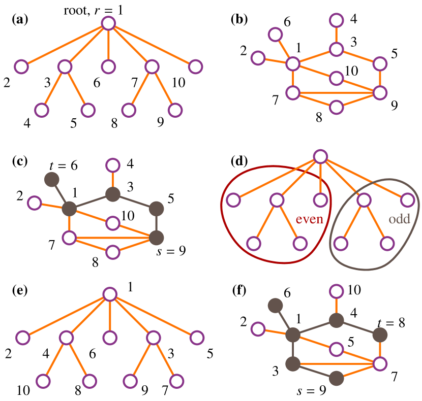
Figure 1: Illustration of the ASD (panels (a)–(c)) and ASU (panels (d)–(f)) indexing and search schemes. (a) shows a search tree where a local search algorithm can find the shortest path from one vertex to another fast. (b) shows a network indexed by the ASD scheme. The tree used in the construction is identical to the one shown in (a). Panel (c) shows an ASD search from $s$ to $t$ (with $\tau=4$). On the way from $t$ to $r$ the packet chooses the neighbor (of the current vertex) with lowest index, which here gives a longer route than the optimal $\{(9,10),(10,1)\}$. (d) shows a possible partition of branches of non-root vertices into classes of as similar size as possible (as done in the ASU indexing scheme). (e) shows a possible indexing based on the partition in (d). Panel (f) displays a search from $s$ to $t$ with $\tau=6$. The shortest path from $t$ to $r$ is accurately found, but a detour to $6$ makes the search from $r$ to $t$ sub-optimal.

II Indexing and search schemes

Now we turn to the schemes for assigning indices to the vertices and using them in search processes. Our two main schemes are both inspired by search trees. Packets first moves towards a root vertex $r$, then towards the destination. Unless the network really is a tree, this approach cannot be exact—a packet is not guaranteed to find the shortest way both from $s$ to $r$ and from $r$ to $t$). However, as we will see, one can assign indices such that the search either from $s$ to $r$, or from $r$ to $t$ is certain to be as short as possible. One of our schemes, ASD (accurate search up), will be such that the shortest upward search is guaranteed, the other, ASD (accurate search down), will have the shortest possible $r$ to $t$ search.

On a technical note, $V$ is a set of distinct elements and an indexing scheme is a bijection $\phi:V\mapsto[1,n]$. In the remainder of the text we will not explicitly distinguish $i\in V$ from $\phi(i)$.

II.1 The ASD indexing and search

The numbers $1,\cdots,n$ can be arranged into a search tree algorithms such that the expected value of $\tau$ scales like $\log n$. In Fig. 1(a) we give an example of a search tree. To go from source $s$ to destination $t$ a packet first moves to the root $r$ by going to the neighbor with lowest index value. From the root to the destination, the package moves to the neighbor with the largest index smaller than, or equal to, $t$. Our strategy for the ASD indexing and search scheme is to construct a spanning tree $T(G)$ for the network; index the tree to make it a search tree; and use the algorithm above to navigate from $s$ to $t$. The problem is, however that real networks are not trees. Imagine adding edges between vertices of the same heights and branches to the tree in Fig. 1(a)—the tree will still be a spanning tree, but the packets may not take the same path from $s$ to $t$ any more. As we will see, with certain ways of constructing the tree and indexing the vertices the search, either from $s$ to $r$ or $r$ to $t$ will be optimal.

We construct $T(G)$ in the following way:

1. Let the root $r$ be a vertex of smallest eccentricity (maximal distance to an other vertex).

2. Construct the tree such that the distances to the root is the same in $T(G)$ and $G$. In other words, such that all edges in $T$ go between different neighborhoods $\Gamma_{l}(r)=\{i\in V:d(i,r)=l$ and $\Gamma_{l+1}(r)\}$ for some level $0\leq l\leq h$, where $h$ is the height of the tree (by the choice of $r$, $h$ is also the radius of the graph). Such a tree can be constructed by finding the set of followed edges in a breadth-first search algorithms starting from $r$.

When it is not clear which vertex, or edge, to choose in the above construction, we choose one at random from all the possible candidates. When $T$ is constructed, let the indices be a preordering of the vertices in $T$ (i.e. the order of first-occurrence of the vertex in a depth-first search of the graph) algorithms .

Now we prove that this indexing and search algorithm always gives the shortest paths from the root to a vertex $t$. Let $E_{T}$ be the edges of $T$ and let $T_{i}$ be the maximal subtree with $i$ as root. By construction, all vertices in $T_{i}$ have indices in $[i,i+|T_{i}|]$ (where $|\;\cdot\;|$ denotes the cardinality of a subgraph). Let $i^{\prime}$ be the largest index in $i$’s neighborhood smaller than $t$. Assume there is an edge $(i,j)\in E\setminus E_{T}$ that the search will follow, i.e. that $i^{\prime}<j<t$. This means that $j\in T_{i^{\prime}}$. By construction, $i^{\prime}$ is the only vertex in $T_{i^{\prime}}$ at a distance $d(r,i^{\prime})$ (the distance from the rest of $T_{i^{\prime}}$ to the root is at least $d(r,i^{\prime})+1$). Since $d(r,i^{\prime})=d(r,i)+1$, we have $d(r,j)\geq d(r,i)+2$ which contradicts the existence of an edge $(i,j)\in E$. Thus searches from $r$ to $t$ will always follow the edges of $T$, which also means the $r$–$t$-searches will be as short as possible.

Searching upwards, from $i$ to $r$, in a graph indexed as above is harder. We know that one shortest path goes via a vertex $j$ with smaller index than $i$, but there might sub-optimal paths via indices $i^{\prime}$ in the intervals $r<i^{\prime}<j$ and $j<i^{\prime}<i$, and there might also be paths via vertices of index larger than $j$, that is optimal. For example, assume the search tree in Fig. 1(a) comes from a graph with the additional edges $(5,9)$, $(8,9)$ and $(9,10)$ (see Fig. 1(b)). Then, the shortest path from $9$ to $r$ via a vertex of lower index is $\{(9,7),(7,1)\}$, but there is an equally long path via a vertex of larger index, $\{(9,10),(10,1)\}$, and longer paths via vertices both smaller and larger than $7$ but smaller than $9$. There thus no general way of finding the shortest way from $s$ to $r$. Instead, we always choose the vertex with the smallest index in the neighborhood. By this strategy a packet will come closer to $r$, in index space, for every step. Furthermore, in tree-like parts of the graph, the search will follow the shortest paths. An illustration of the ASD search can be found in Fig. 1(c).

II.2 The ASU indexing and search

Consider a tree $T(G)$ constructed as in the previous section and an indexing such that $d(i,r)<d(j,r)$ implies $i<j$ (i.e., all indices of a level further from the root is larger than in levels closer to $r$). With such an indexing, since the neighbor of a vertex with the smallest index necessarily is one step closer to the root, a packet can always find one shortest way too the root. But once the package is at the root the indices is not of so much help. The search from $r$ to $t$ has to be, essentially, a depth-first search. There are, however, a few tricks to speed up the search. First, there is no need to search deeper than $t$—if $j>t$, then $t\notin T_{j}$. Second, one can choose the indices $i,\cdots,i+|\Gamma_{l}(r)|$ of one level in the tree in a way to narrow down the search. For example, one can divide the vertices into $\nu$ classes (defined by e.g. the remainder when the index is divided by $\nu$) and index vertices of connected regions of the graph with indices of the same class. The search can then be restricted to the same class as the destination. We will pursue this idea with $\nu=2$.

To derive the ASU indexing scheme, the first goal is to divide the vertices into classes of connected subgraphs. Furthermore, we require all classes to be connected to the root vertex. Another aim is to make the classes of as similar sizes as possible. Our first step is to make $k_{r}$ (the degree, or number of neighbors, of $r$) parallel depth-first searches. Second we group the $k_{r}$ search trees into $\nu$ groups with maximally similar sizes. In our case, we seek a partition of the search trees into two classes such that the sums of vertices in the respective classes are as close as possible. Then we go through the levels, starting from the root, and assign numbers such that vertices of one partition have even indices, while the other has odd numbers (this assignment might not always work). To avoid systematic errors we sample the elements of levels randomly. This construction scheme is illustrated in Fig. 1(d) and (e).

II.3 Degree-based and random search

As a reference, we also run simulations for two depth-first search methods that do not utilize indices ada:se2 . One of them, Rnd, is regular depth-first search where the neighbors are traversed in random order. In the other, Deg, the neighbors are chosen in order from high to low degree. Just like for ASU and ASD methods, a packet is assumed to have knowledge about its neighborhood—if the destination is in the neighborhood of a vertex, then the search will be over the next time step.

III Network models

The efficiency of our indexing and search schemes are more or less directly affected by the network structure. To investigate this relationship we test the search schemes on four different types of network models: modified Erdős–Rényi (ER) graphs er:on , square lattices, Barabási–Albert (BA) ba:model and Holme–Kim (HK) hk:model networks. To facilitate comparison, we have the same average degree, four (dictated by the square grid), in all networks.

III.1 Modified ER graphs

The ER model is the simplest model for randomly generating simple graphs with $n$ vertices and $m$ edges. The edges are added one by one to randomly chosen vertex pairs (the only restriction being that loops or multiple edges are not allowed). A problem for our purpose is that ER graphs are not necessarily connected (something required to measure $\bar{\tau}$). To remedy this we propose a scheme to make networks connected.

1. Detect the connected components.

2. Go through the connected components sequentially. Denote the current component $C_{I}$.

   1. Pick a component $C_{J}$ randomly.

   2. Pick a random edge $(i,j)$ whose removal would not fragment $C_{J}$. If no such edge exist, go to step 2.

   3. Pick a random vertex $i^{\prime}$ of $C_{I}$.

   4. Replace $(i,j)$ by $(i^{\prime},j)$. If the edge $(i^{\prime},j)$ would exist already (an unlikely event), go to step 2d. If there is no vertex $i^{\prime}\in C_{I}$ such that $(i^{\prime},j)$ does not already exist, then go to 2.

3. If the network is disconnected still, go to step 1.

In practice, even for our largest system sizes, the above algorithm converges in a few iterations. The number of edges needed to be added never exceed a few percent of $m$, and this addition is made with greatest possible randomness; hence we believe the essential network structure of the ER model is conserved.

III.2 Square lattice

We use square lattices with periodic boundary conditions. $n$ vertices spread out regularly on a $L\times L$-grid such that the vertex with coordinates $(x,y)$, $1\leq x,y\leq L$, is connected to $(x,y+1)$, $(x+1,y)$, $(x,y-1)$, $(x-1,y)$ (if $x=1$, we formally let $x-1=L$, if $x=L$ we let $x+1$ represent $1$; and correspondingly for $y$).

III.3 BA model

The popular BA model ba:model of networks with a power-law degree distribution works as follows (with our parameter settings). Start with one vertex connected to two degree-one vertices. Iteratively add vertices connected to two other vertices. Let the probability of connecting the new vertex to a vertex $i$ already present in the network is proportional to $k_{i}$ (so called preferential attachment).

III.4 HK model

The HK model hk:model is a modification of the BA model to give the network higher number of triangles. When edges are added from the new vertex to already present vertices, the first edge is added by preferential attachment. The second edge is added to one of $i$’s neighbors, forming a triangle.

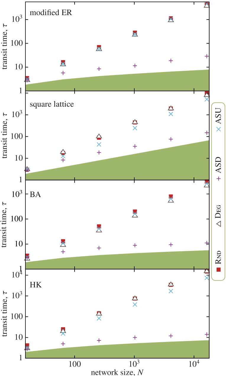
Figure 2: The average search time $\bar{\tau}$ as a function of the graph sizes $n$. In all panels, we display data for the different indexing and search schemes. The shaded areas are unreachable (corresponding to $\bar{\tau}$ values smaller than the theoretical minimum—the average distance $\bar{d}$). The different panels correspond to the modified ER model, square grid, BA model and HK model networks respectively. Error bars would have been smaller than the symbol sizes.

IV Numerical results

We study the search schemes on the four different network topologies numerically. We use $100$ independent networks and $100$ different $s$–$t$-pairs for every network. The network sizes range from $n=16$ to $n=16{,}384$.

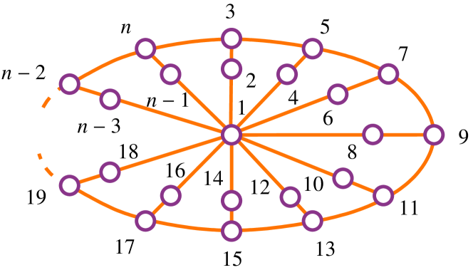
Figure 3: A worst case scenario for navigating from $s$ to $r$ with the ASD indexing and search scheme. A packet from $n-2$ to $1$ will travel along the perimeter to $3$ and then move towards the center.

In Fig. 2 we display the average search times as a function of system size for our simulations. The most conspicuous feature is that the ASD scheme is always, by far, the most efficient. While ASU and Deg are close to the least efficient method (Rnd), ASD is rather close to the theoretical limit (equal to the average distances $\bar{\tau}$—the upper border of the shaded areas in Fig. 2). To be more precise, $\bar{\tau}$ is quite constant, about two times larger than the average distance. The other search schemes (ASU, Deg and Rnd) follow faster increasing functional forms. For the square lattice, these three schemes increase, approximately proportional to $n$ (the analytical value for two-dimensional random walks) whereas for ASD, $\bar{\tau}$ scale like distances in square grids, $n^{1/2}$. One way of interpreting this result is that while ASD manages to find the root as fast as it finds the destination from the root, ASU fails to find $t$ faster than a random search. The slow downward performance of ASU is not unexpected—the $r$–$t$-search in ASU only differs from a random depth-first search in that it does not search further than the level of the destination, and that it restricts the search-space to half its original size by dividing the vertices into odd and even indices. The fast upward search of ASD is more surprising. In Fig. 3 we show a network where ASD performs badly. The average time to search upwards is $(n^{2}+20n-13)/8n\rightarrow n/8$ as $n\rightarrow\infty$. The downward search takes $3(n-1)/2n\sim 3/2$ giving a total expected value of $\bar{\tau}\sim n/8$. This can be compared to the average distance $\bar{d}=3-21/4n+2/n^{2}\sim 3$. For this example, $\bar{\tau}$ and $\bar{d}$ diverge in a way not seen in the network models. Why is the search so much faster in the model networks? One point is that the worst-case indexing seen in Fig. 3 is very unlikely. Since the spokes would be sampled randomly, the chance that a vertex at the perimeter not finds $r$ in two steps is $1/2$, the probability of a perimeter vertex to find $r$ in $3$ steps is $1/4$, and so on. Carrying on this calculation, a vertex at the perimeter reaches $r$ in $2\sum_{k}k2^{k}+2\sim 6$ timesteps giving $\bar{\tau}\sim 5$—not too far from the observed $\bar{\tau}/\bar{d}\sim 2$. We note however that for the model networks many other factors that are not present in the wheel-graph of Fig. 3 affect $\bar{\tau}$. For example, the high density of short triangles in the HK model networks will introduce many edges between vertices of the same level in $T(G)$ which will affect the search efficiency.

$\bar{\tau}$ is approximately linear for the ASU, Deg and Rnd on all network models. The slopes of these curves are, however, a little different. First, the Deg method is more efficient (compared to ASU and Rnd) for BA networks, than for the modified ER model. This observation (also made in Ref. ada:se2 ) can be explained by the skewed degree distribution in the BA-network—the packet reaches high-degree vertices fast. The packet can see a large part of the network from these hubs, and is therefore more likely to see $t$. More interesting, perhaps, is that ASU is more efficient for the networks with a higher density of short cycles (the square lattice and HK models). A rough explanation is that the partition procedure of ASU cuts off many edges between vertices at the same distance from $r$. Since there are many such edges in these network models, the network will effectively be sparser (without changing $G$’s diameter), which results in a better performance.

V Discussion

We have investigated navigation in valued graphs, more specifically in indexed graphs—graphs where every vertex is associated with a unique number in the interval $[1,n]$. These indices can be assigned to facilitate the packet navigation. The packets are assumed to have no a priori knowledge about the network, except the neighborhoods of their current positions, but memory enough to perform a depth-first search. We find that one of our investigated methods, ASD, is very efficient for four topologically very different network models. The searches with the ASD scheme are roughly twice as long as the shortest paths (scaling in the same way as the average distance).

Navigation on indexed graphs has applications in distributed information systems. If, specifically, the amount of information that can be stored at the vertices were limited, search strategies such as ours would be useful. One such system is the Autonomous System level Internet where the information stored at each vertex (with the current protocols) increase at least as fast as the networks themselves. For most real-world applications (other examples being ad hoc networksadhoc or peer-to-peer networks sarshar ; niloy ; mejngg:p2p ) there are additional constraints so that the algorithms of this paper cannot immediately be applied. Such networks are typically changing over time, so the indexing should ideally be possible to be extended on the fly as vertices and edges are added and deleted from the network. Apart from this, a future direction for research on indexed graphs is to improve the performance of the algorithms presented in this work. There might be search-tree based algorithm that neither finds the shortest path to the root, nor finds the shortest way to the destination. For some network topologies there might be faster algorithms that are not based on constructing a spanning tree. Consider, for example, modular networks mejn:commu (i.e. networks with tightly connected subgraphs that are only sparsely interconnected) in such networks the search can be divided into two stages—first find the cluster of the destination, then the destination. These two stages should be reflected in a fast navigation algorithm.

- (1) L. A. Adamic, R. M. Lukose, A. R. Puniyani, and B. A. Huberman. Search in power-law networks. Phys. Rev. E, 64:046135, 2001.
- (2) A.-L. Barabási and R. Albert. Emergence of scaling in random networks. Science, 286:509–512, 1999.
- (3) T. H. Cormen, C. E. Leiserson, R. L. Rivest, and C. Stein. Introduction to Algorithms. The MIT Press, Cambridge MA, 2nd edition, 2001.
- (4) C. de Morais Cordeiro and D. P. Agrawal. Ad Hoc & Sensor Networks: Theory and Applications. World Scientific, Hackensack, NJ, 2006.
- (5) P. Erdős and A. Rényi. On random graphs I. Publ. Math. Debrecen, 6:290–297, 1959.
- (6) N. Ganguly, L. Brusch, and A. Deutsch. Design and analysis of a bio-inspired search algorithm for peer to peer networks. In O. Babaoglu, M. Jelasity, A. Montresor, C. Fetzer, and S. Leonardi, editors, Self-star Properties in Complex Information Systems, pages 358–372, New York, 2007. Springer-Verlag.
- (7) G. Ghoshal and M. E. J. Newman. Growing distributed networks with arbitrary degree distributions. e-print physics/0608057.
- (8) P. Holme and B. J. Kim. Growing scale-free networks with tunable clustering. Phys. Rev. E, 65:026107, 2002.
- (9) B. J. Kim, C. N. Yoon, S. K. Han, and H. Jeong. Path finding strategies in scale-free networks. Phys. Rev. E, 65:027103, 2002.
- (10) J. M. Kleinberg. Navigation in a small world. Nature, 406:845, 2000.
- (11) M. E. J. Newman and M. Girvan. Finding and evaluating community structure in networks. Phys. Rev. E, 69:026113, 2004.
- (12) N. Sarshar, P. O. Boykin, and V. P. Roychowdhury. Percolation search in power law networks: Making unstructured peer-to-peer networks scalable. In Proceedings of Fourth International Conference on Peer-to-Peer Computing, pages 2–9. IEEE, 2004.
- (13) P. Sen. A novel approach for studying realistic navigations on networks. J. Stat. Mech., P04007, 2007.
- (14) H. Zhu and Z.-X. Huang. Navigation in a small world with local information. Phys. Rev. E, 70:036117, 2004.