Inference by replication in densely connected systems

Abstract

An efficient Bayesian inference method for problems that can be mapped onto dense graphs is presented. The approach is based on message passing where messages are averaged over a large number of replicated variable systems exposed to the same evidential nodes. An assumption about the symmetry of the solutions is required for carrying out the averages; here we extend the previous derivation based on a replica symmetric (RS) like structure to include a more complex one-step replica symmetry breaking (1RSB)-like ansatz. To demonstrate the potential of the approach it is employed for studying critical properties of the Ising linear perceptron and for multiuser detection in Code Division Multiple Access (CDMA) under different noise models. Results obtained under the RS assumption in the non-critical regime give rise to a highly efficient signal detection algorithm in the context of CDMA; while in the critical regime one observes a first order transition line that ends in a continuous phase transition point. Finite size effects are also observed. While the 1RSB ansatz is not required for the original problems, it was applied to the CDMA signal detection problem with a more complex noise model that exhibits RSB behaviour, resulting in an improvement in performance.

I Introduction

Efficient inference in large complex systems is a major challenge with significant implications in science, engineering and computing. Exact inference is computationally hard in complex systems and a range of approximation methods have been devised over the years, many of which have been originated in the physics literature MPV . A recent review MFAbook highlights the links between the various approximation methods and their applications.

Approximative Bayesian inference techniques arguably offer the most principled approach to information extraction, by combining a rigorous statistical approach with a feasible but systematic approximation. Although message passing techniques have existed for some time in the computer science community Pearl ; Jensen they have enjoyed growing popularity in recent years macKay , mainly within the context of Bayesian networks and the use of Belief Propagation (BP) for a range of inference applications, from signal extraction in telecommunication to machine learning.

The main advantage of these techniques is their moderate growth in computational cost, with respect to the systems size, due to the local nature of the calculation when applied to sparse graphs. Until recently, message passing techniques were deemed unsuitable for inference in densely connected systems due to the inherently high number of short loops in the corresponding graphical representation, and the large number of connections per node, which results in a high computational cost. Both properties are considered prohibitive to the use of conventional message passing techniques in such problems.

A recently suggested method for message passing in densely connected systems KabashimaCDMA relies on replacing individual messages by averages sampled from a Gaussian distribution of some mean and variance that are modified iteratively. The method has been applied for the CDMA signal detection inference problem; it successfully finds optimal solutions where the space of solutions is contiguous but breaks down when the solution space becomes fragmented, for instance, when there is a mismatch between the true and assumed noise levels in the CDMA detection problem. The emergence of competing solutions gives rise to conflicting messages that result in bungled average messages and suboptimal performance. In statistical physics terms, it corresponds to the replica symmetric solution in dense systems Nishimoribook and gives poor estimates when more complex solution structures are required.

In the current paper, we methodologically extend the approach of Kabashima KabashimaCDMA for inference in dense graphs by considering a large (infinite) number of replicated variable systems, exposed to the same evidential data (received signals). Each one of the systems represents a pure state and a possible solution. The pseudo posteriors, that form the basis for our estimates, are based on averages over the replicated systems. The method has been employed previously only in the non-critical regime neirottisaad , using the most basic (RS-like) ansatz for the solution structure. In the current paper we study both critical and non-critical regimes and extend the solution structure considered to include step replica symmetry breaking (1RSB) like structures footnote . To demonstrate the potential of this approach and the performance obtained using the resulting algorithm we apply the method to two different but related problems: signal detection in Code Division Multiple Access (CDMA) and learning in the Ising linear perceptron (ILP). ​​

We investigate both RS and 1RSB-like structures. The former is applied to both CDMA and ILP problems and seems to be sufficient for obtaining optimal performances; the latter is applied to a variant of the CDMA signal detection problem with a more complex noise model that exhibits RSB-like behaviour, to demonstrate its efficacy for particularly difficult inference tasks.

In section II we will introduce the general models studied, followed by a brief review of message passing techniques for dense systems in section III. The general derivation of our approach, for both RS and RSB-like solution structures, will be presented in section IV; numerical studies of both CDMA signal detection and ILP learning will be reported in section V. To demonstrate the method based on the more complex 1RSB solution structure, and to examine its efficacy to problems that require such structures, we will introduce a variant of the CDMA signal detection problem and study it numerically in section VI. We will conclude the presentation with a summary and point to future research directions. Details of the derivation will be provided in Appendices A-E.

II Models studied

Before describing the inference method, the approach taken and the algorithms derived from it, it would be helpful to briefly describe the exemplar inference problems tackled in this paper.

We apply the method to two different but related inference problems: signal detection in CDMA and learning in the Ising linear perceptron (ILP). Both correspond to inference problems where data points are noisy representations of sums of binary variables modulated by random binary values.

Multiple access communication refers to the transmission of multiple messages to a single receiver. The scenario we study here, described schematically in figure 1(a), is that of $K$ users transmitting independent messages over an additive white Gaussian noise (AWGN) channel of zero mean and variance $\sigma_{0}^{2}$. Various methods are in place for separating the messages, in particular Time, Frequency and Code Division Multiple Access CDMAbook . The latter, is based on spreading the signal by using $K$ individual random binary spreading codes of spreading factor $N$. We consider the large-system limit, in which the number of users $K$ tends to infinity while the system load $\beta\equiv K/N$ is kept to be $\mathcal{O}(1)$. We focus on a CDMA system using binary phase shift keying (BPSK) symbols and will assume the power is completely controlled to unit energy. The received aggregated, modulated and corrupted signal is of the form:

$$y_{\mu}=\frac{1}{\sqrt{N}}\sum_{k=1}^{K}s_{\mu k}b_{k}+\sigma_{0}n_{\mu}$$ (1)

where $b_{k}$ is the bit transmitted by user $k$, $s_{\mu k}$ is the spreading chip value, $n_{\mu}$ is the Gaussian noise variable drawn from $\mathcal{N}\left(0,1\right)$, and $y_{\mu}$ the received message. The task is to infer the original transmission from the set of received messages. This process is reminiscent of the learning task performed by a perceptron with binary weights and linear output, which is the next example considered in this paper.

Learning in neural networks has attracted considerable theoretical interest. In particular we focus on supervised learning from examples, which relies on a training set consisting of examples of the target task Seung . We consider a perceptron, described schematically in figure 1(b), which is a network that sums a single layer of inputs $s_{\mu k}$ with synaptic weights $b_{k}$ and passes the result through a transfer function $y_{\mu}$

$$y_{\mu}=g\left(\frac{1}{\sqrt{K}}\sum_{k=1}^{K}s_{\mu k}b_{k}\right)\,,$$ (2)

where $g$ is typically a non-linear sigmoidal function. If $g(x)=x$ the network is termed linear output perceptron. If the weights $b_{k}\in\left\{\pm 1\right\}$ the network is called Ising perceptron. Learning is a search through the weight space for the perceptron that best approximates a target rule.

The similarity between the linear perceptron of equation (2) and the CDMA detection problem of Eq.(1) allows for a direct relation between the two problems to be established. The main difference between the problems is the regime of interest. While CDMA detection applications are of interest mainly for non-critical low load values, ILP studies focused on the critical regime. We consider both regimes in this paper. ​​

Figure 1: Schematic representation of (a) the CDMA system. (b) the ILP.

III Message passing for inference in densely connected systems

Graphical models (Bayes belief networks) provide a powerful framework for modelling statistical dependencies between variables Pearl ; Jensen ; macKay . They play an essential role in devising a principled probabilistic framework for inference in a broad range of applications.

Message passing techniques are typically used for inference in graphical models that can be represented by a sparse graph with a few (typically long) loops. They are aimed at obtaining (pseudo) posterior estimates for the system’s variables by iteratively passing messages (locally calculated conditional probabilities) between variables. Iterative message passing of this type is guaranteed to converge to the globally correct estimate when the system is tree-like; there are no such guarantees for systems with loops even in the case of large loops and a local tree-like structure (although message passing techniques have been used successfully in loopy systems, supported by some limited theory weiss ). A clear link has been established between certain message passing algorithms and well known methods of statistical mechanics MFAbook such as the Bethe approximation TAPEPL ; YFW .

These inherent limitations seem to prevent the use of message passing techniques in densely connected systems due to their high connectivity, implying an exponentially growing cost, and an exponential number of loops. However, an exciting new approach has been recently suggested KabashimaCDMA for extending BP techniques Pearl ; Jensen ; macKay to densely connected systems. In this approach, messages are grouped together, giving rise to a macroscopic random variable, drawn from a Gaussian distribution of varying mean and variance for each of the nodes. The technique has been successfully applied to CDMA signal detection problems and the results reported are competitive with those of other state-of-the-art techniques. However, the current approach has some inherent limitations KabashimaCDMA , presumably due to its similarity to the replica symmetric solution in the equivalent Ising spin models MPV ; Nishimoribook .

In a separate recent development MPZ , the replica-symmetric-equivalent BP has been extended to Survey Propagation (SP), which corresponds to one-step replica symmetry breaking in diluted systems. This new algorithm, motivated by the theoretical physics interpretation of such problems, has been highly successful in solving hard computational problems MPZ , far beyond other existing approaches. In addition, the algorithm facilitated theoretical studies of the corresponding physical system and contributed to our understanding of it MZPRE . The SP algorithm has recently been modified to handle Ising and multilayer perceptrons BZ .

​​

IV General Formalism

We recently presented a new approach neirottisaad for inference in densely connected systems, which was inspired by both the extension of BP to densely connected graphs and the introduction of SP. The systems we consider here are characterised by multiplicity of pure states and a possible fragmentation of the space of solutions. To address the inference problem in such cases we consider an ensemble of replicated systems where averages are taken over the ensemble of potential solutions. This amounts to the presentation of a new graph, where the observables $y_{\mu}$ are linked to variables in all replicated systems, namely $\mathbf{B}\!=\!\left(\mathbf{b}^{1},\mathbf{b}^{2},\dots,\mathbf{b}^{n}\right)$; where $\mathbf{b}^{{\textrm{a}}}\!=\!\left(b_{1}^{{\textrm{a}}},b_{2}^{{\textrm{a}}},\dots,b_{K}^{{\textrm{a}}}\right)^{\textsf{T}}$, as shown in figure 2. To estimate the variables $\mathbf{B}$ given the data $\mathbf{y^{\sf T}}\!=\!\left(y_{1},y_{2},\ldots,y_{N}\right)$, in a Bayesian framework, we have to maximise the posterior $P\left(\mathbf{B}|\mathbf{y}\right)\!\propto\!\prod_{\mu=1}^{N}P\left(y_{\mu}|\mathbf{B}\right)P\left(\mathbf{B}\right),$ where we have considered independent data, and thus $P\left(\mathbf{y}|\mathbf{B}\right)\!=\!\prod_{\mu=1}^{N}P\left(y_{\mu}|\mathbf{B}\right)$.

The likelihood so defined is of a general form; the explicit expression depends on the particular problem studied. Here, we are interested in cases where $\mathbf{b}\!\in\!\left\{\pm 1\right\}^{K}$ is an unbiased vector and $P\left(\mathbf{B}\right)\!=\!2^{-Kn}$. The estimate we would like to obtain is the maximiser of the posterior marginal (MPM) $\widehat{\mathbf{b}}_{k}\!=\!\mathop{\mathrm{missing}}{argmax}_{\mathbf{b}_{k}\in\left\{\pm 1\right\}^{n}}\sum_{\left\{\mathbf{b}_{l\neq k}\right\}}P\left(\mathbf{B}|\mathbf{y}\right)\,\,,$ which is expected to be a vector with equal entries for all replica $\widehat{b}_{k}^{1}=\widehat{b}_{k}^{2}=\dots=\widehat{b}_{k}^{n}$. The number of operations required to obtain the full MPM estimator is of $\mathcal{O}\left(2^{K}\right)$ which is infeasible for large $K$ values.

To obtain an approximate MPM estimate we apply BP message passing technique Pearl ; Jensen ; macKay . In particular we are interested here in the application of BP to densely connected graphs, similar to the one presented in KabashimaCDMA . The latter is based on estimating a single solution and therefore does not converge, as has been observed, when the solution space becomes fragmented and multiple solutions emerge. This arguably corresponds to the replica symmetry breaking phenomena and occurs, for instance, when the noise level is unknown in the CDMA signal detection case.

A potential algorithmic improvement is achieved by the introduction of an SP-like approach, based on replicated variable systems, similar to the approach taken in problems that can be mapped onto sparsely connected graphs.

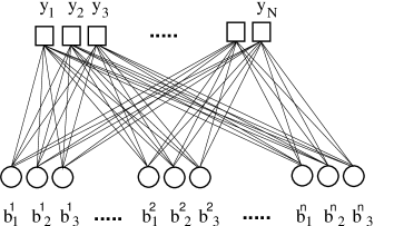
Figure 2: Replicated solutions $\mathbf{B}\!=\!\left(\mathbf{b}_{1},\,\mathbf{b}_{2},..,\mathbf{b}_{K}\right)$ given data.

Using Bayes rule one straightforwardly obtains the BP equations:

$$P^{t+1}\left(y_{\mu}|\mathbf{b}_{k},\left\{y_{\nu\neq\mu}\right\}\right) = \sum_{\left\{\mathbf{b}_{l\neq k}\right\}}P\left(y_{\mu}|\mathbf{B}\right)\prod_{l\neq k}P^{t}\left(\mathbf{b}_{l}|\left\{y_{\nu\neq\mu}\right\}\right)$$ (3)

$$P^{t}\left(\mathbf{b}_{l}|\left\{y_{\nu\neq\mu}\right\}\right) \propto \prod_{\nu\neq\mu}P^{t}\left(y_{\nu}|\mathbf{b}_{l},\left\{y_{\sigma\neq\nu}\right\}\right)\,.$$ (4)

For calculating the posterior $P\left(\mathbf{y}|\mathbf{B}\right),$ we assume a dependency of the data on the parameters of the form $y_{\mu}=\mathcal{F}\left(\sum_{l=1}^{K}\varepsilon_{\mu l}\mathbf{b}_{l};\mathbold{\gamma}\right)$, where $\mathcal{F}$ is some general smooth function, $\mathbold{\gamma}$ are model parameters and $\varepsilon_{\mu l}$ are small enough to ensure that $\sum_{l=1}^{K}\varepsilon_{\mu l}b_{l}^{{\rm a}}\sim\mathcal{O}(1)$. We define the vector $\mathbf{{\Delta}}_{\mu}\equiv\sum_{l=1}^{K}\varepsilon_{\mu l}\mathbf{b}_{l}=\sum_{l\neq k}\varepsilon_{\mu l}\mathbf{b}_{l}+\varepsilon_{\mu k}\mathbf{b}_{k}=\mathbf{{\Delta}}_{\mu k}+\varepsilon_{\mu k}\mathbf{b}_{k}.$ Thus, using $y_{\mu}=\mathcal{F}\left(\mathbf{{\Delta}}_{\mu k}+\varepsilon_{\mu k}\mathbf{b}_{k};\mathbold{\gamma}\right)$ we can model the likelihood such that

$$P\left(y_{\mu}|\mathbf{B}\right) = \int{\rm d}\mathbf{{\Delta}}_{\mu k}P\left(y_{\mu},\mathbf{{\Delta}}_{\mu k}|\mathbf{B};\mathbold{\gamma}\right)$$ (5)

$$= \int{\rm d}\mathbf{{\Delta}}_{\mu k}P\left(y_{\mu}|\mathbf{{\Delta}}_{\mu k},\mathbf{B};\mathbold{\gamma}\right)P\left(\mathbf{{\Delta}}_{\mu k}|\mathbf{B}\right)$$

$$= \int{\rm d}\mathbf{{\Delta}}_{\mu k}P\left(y_{\mu}|\mathbf{{\Delta}}_{\mu k}+\varepsilon_{\mu k}\mathbf{b}_{k};\mathbold{\gamma}\right)P\left(\mathbf{{\Delta}}_{\mu k}|\mathbf{B}\right)$$

$$\simeq \int{\rm d}\mathbf{{\Delta}}_{\mu k}\left[1+\varepsilon_{\mu k}\mathbf{b}_{k}^{\sf T}\nabla_{\mathbf{{\Delta}}_{\mu k}}\ln P\left(y_{\mu}|\mathbf{{\Delta}}_{\mu k};\mathbold{\gamma}\right)\right]P\left(y_{\mu}|\mathbf{{\Delta}}_{\mu k};\mathbold{\gamma}\right)\,P\left(\mathbf{{\Delta}}_{\mu k}|\mathbf{B}\right)\,,$$

where we have assumed that $P\left(y_{\mu}|\mathbf{{\Delta}}_{\mu k},\mathbf{B};\mathbold{\gamma}\right)\approx P\left(y_{\mu}|\mathbf{{\Delta}}_{\mu k}+\varepsilon_{\mu k}\mathbf{b}_{k};\mathbold{\gamma}\right)$,

due to the assumed dependence of the observed values $y_{\mu}$ on $\mathbf{\Delta}_{\mu k}$ and $\mathbf{b}_{k}$.

IV.1 Inter-replica correlations

An explicit expression for inter-dependence between solutions is required for obtaining a closed set of update equations. We assume a dependence of the form

$$P^{t}\left(\mathbf{b}_{k}\left|\left\{y_{\nu\neq\mu}\right\}\right.\right)\propto\exp\left\{\mathbf{h}_{\mu k}^{t\mathsf{T}}\,\mathbf{b}_{k}+\frac{1}{2}\mathbf{b}_{k}^{\textsf{T}}\mathbf{Q}_{\mu k}^{t}\,\mathbf{b}_{k}\right\},$$ (6)

where $\mathbf{h}_{\mu k}^{t}$ is a vector representing an external field and $\mathbf{Q}_{\mu k}^{t}$ the matrix of cross-replica interaction. The form of $\mathbf{Q}_{\mu k}^{t}$ depends upon the particular case considered. We assume one of the following symmetry relation between the replicated solutions:

$$\left(\mathbf{h}_{\mu k}^{t}\right)^{\ell{\rm a}} = h_{\mu k}^{t},\leavevmode\nobreak\ \mbox{\leavevmode\nobreak\ \leavevmode\nobreak\ \leavevmode\nobreak\ \leavevmode\nobreak\ and\leavevmode\nobreak\ \leavevmode\nobreak\ }$$

$$\left({}^{{\rm(RS)}}\mathbf{Q}_{\mu k}^{t}\right)^{\mathrm{a}{\rm a}^{\prime}} = \delta^{\mathrm{a}{\rm a}^{\prime}}\,q_{0\mu k}^{t}+\left(1-\delta^{{\rm a}{\rm a}^{\prime}}\right)\,q_{1\mu k}^{t}\leavevmode\nobreak\ \mbox{\leavevmode\nobreak\ \leavevmode\nobreak\ or\leavevmode\nobreak\ \leavevmode\nobreak\ }$$

$$\left({}^{{\rm(1RSB)}}\mathbf{Q}_{\mu k}^{t}\right)^{\ell{\rm a}\;\ell^{\prime}{\rm a}^{\prime}} = \delta^{\ell\ell^{\prime}}\left({}^{{\rm(RS)}}\mathbf{Q}_{\mu k}^{t}\right)^{\mathrm{a}{\rm a}^{\prime}}+\left(1-\delta^{\ell\ell^{\prime}}\right)q_{2\mu k}^{t}\,,$$

where $\ell$ is a block index that runs from 1 to $L$ and ‘a’ is a intra-block replica index that runs form 1 to $n$ where $n$ is the number of variables per block. We also make the following reasonable assumption $q_{0\mu k}^{t}>q_{1\mu k}^{t}>q_{2\mu k}^{t}>0$, as one expects correlations to gradually decrease between variables with non-identical replica and block indices, respectively.

For both types of symmetries considered, the correlation matrix defined as:

$$\left(\mathbf{\Upsilon}_{\mu k}^{t}\right)^{\sf\mathbf{I}\;\sf\mathbf{I}^{\prime}}\equiv\left\langle\Delta_{\mu k}^{\sf\mathbf{I}}\Delta_{\mu k}^{\sf\mathbf{I}^{\prime}}\right\rangle-\left\langle\Delta_{\mu k}^{\sf\mathbf{I}^{\phantom{\prime}}}\right\rangle\left\langle\Delta_{\mu k}^{\sf\mathbf{I}^{\prime}}\right\rangle\,$$

where $\sf\mathbf{I}$ is an index or a pair of indices for RS and 1RSB, respectively. The correlation matrix is assumed to be self-averaging, i.e. $\mathbf{\Upsilon}_{\mu k}^{t}\simeq\mathbf{\Upsilon}^{t}$ and preserves the symmetry of the matrix $\mathbf{Q}_{\mu k}^{t}$. An explicit derivation of the entries of $\mathbf{\Upsilon}^{t}$ is presented in Appendices A and B, for the RS and RSB-like correlation structures, respectively; the matrices take following the general form:

$$\left({}^{{\rm(RS)}}\mathbf{\Upsilon}^{t}\right)^{{\rm a}{\rm a}^{\prime}} = \delta^{{\rm a}{\rm a}^{\prime}}X^{t}+\left(1-\delta^{{\rm a}{\rm a}^{\prime}}\right)\frac{1}{n}R^{t}$$

$$\left({}^{{\rm(1RSB)}}\mathbf{\Upsilon}^{t}\right)^{{\rm a}\ell\;{\rm a}^{\prime}\ell^{\prime}} = \delta^{\ell\ell^{\prime}}\left[\delta^{{\rm a}{\rm a}^{\prime}}X^{t}+\left(1-\delta^{{\rm a}{\rm a}^{\prime}}\right)\frac{1}{n}V^{t}\right]+\left(1-\delta^{\ell\ell^{\prime}}\right)\frac{1}{nL}\left(V^{t}-R^{t}\right)\,.$$

Thus, for the appropriate centre of the distribution $\mathbf{u}_{\mu k}^{t}$ (see equations  (31) and (45)), the probability of $\mathbf{{\Delta}}_{\mu k}$ can be expressed as:

$$P\left(\mathbf{{\Delta}}_{\mu k}|\mathbf{B}\right) = \sqrt{\frac{1}{\left(2\pi\right)^{n}\det\left(\mathbf{\Upsilon}^{t}\right)}}\exp\left\{-\frac{1}{2}\left(\mathbf{{\Delta}}_{\mu k}-\mathbf{u}_{\mu k}^{t}\right)^{\mathsf{T}}\left(\mathbf{\Upsilon}^{t}\right)^{-1}\left(\mathbf{{\Delta}}_{\mu k}-\mathbf{u}_{\mu k}^{t}\right)\right\}$$

$$\propto {\small\begin{cases}\int{\rm d}\vartheta\,\exp\left\{-n\,{\displaystyle\frac{\left(\vartheta-u_{\mu k}^{t}\right)^{2}}{2R^{t}}}\right\}\prod_{{\rm a}=1}^{n}\exp\left\{-{\displaystyle\frac{\left(\Delta_{\mu k}^{{\rm a}}-\vartheta\right)^{2}}{2X^{t}}}\right\}&\mbox{(RS)}\\ \int{\rm d}\mathbf{{\Theta}}\,\prod_{\ell=1}^{L}\exp\left\{-{\displaystyle\frac{n}{2}\left[\frac{\left(\vartheta^{0}\right)^{2}}{V^{t}-R^{t}}+\frac{\left(\vartheta^{\ell}\right)^{2}}{V^{t}-L^{-1}\left(V^{t}-R^{t}\right)}\right]}\right\}\prod_{{\rm a}=1}^{n}\exp\left\{-{\displaystyle\frac{\left(\Delta_{\mu k}^{\ell{\rm a}}-\vartheta_{\mu k}^{0\ell t}\right)^{2}}{2\left(X^{t}-n^{-1}V^{t}\right)}}\right\}&\mbox{(RSB)}\end{cases}}$$

for the RS and RSB-like correlation matrices, respectively, where $\vartheta_{\mu k}^{0\ell t}\equiv\vartheta^{0}+\vartheta^{\ell}+u_{\mu k}^{t}$ and $\mathbf{{\Theta}}^{\sf T}=\left(\vartheta^{0},\vartheta^{1},\dots,\vartheta^{L}\right).$

IV.2 Messages

Having obtained the conditional probability distribution $P\left(\mathbf{{\Delta}}_{\mu k}|\mathbf{B}\right)$ one can then derive explicit expressions for the messages $m_{\mu k}$ (magnetisation) and $\widehat{m}_{\mu k}$ that can be viewed as parameters in the corresponding marginalised binary distributions $P^{t}\left(y_{\mu}|b_{k},\{y_{\nu\neq\mu}\}\right)\propto(1+\hat{m}_{\mu k}^{t}b_{k})/2$ and $P^{t}\left(b_{k}|\{y_{\nu\neq\mu}\}\right)=(1+m_{\mu k}^{t}b_{k})/2$.

The messages from nodes $y_{\mu}$ to nodes $\mathbf{b}_{k}$, as derived in Appendix C, equations (C)-(53)

$$\widehat{m}_{\mu k}^{t+1} = \begin{cases}\varepsilon_{\mu k}{\displaystyle\frac{\tilde{\vartheta}_{\mu k}^{t}-u_{\mu k}^{t}}{R^{t}}}&\mbox{(RS)}\\ \varepsilon_{\mu k}{\displaystyle\frac{\tilde{\vartheta}_{\mu k}^{t}-u_{\mu k}^{t}}{2V^{t}-R^{t}}+\frac{\varepsilon_{\mu k}}{2n}\,\frac{\mathcal{P}_{2}V^{t}}{1-\mathcal{P}_{1}V^{t}}\,}&\mbox{(RSB)}\end{cases},$$ (8)

where $\mathcal{P}_{j}=\left.{\displaystyle\frac{\partial^{j}\mathcal{P}}{\partial\vartheta^{j}}}\right|_{\vartheta=\tilde{\vartheta}_{\mu k}^{t}}$, $\mathcal{P}$ is defined in equation (48) and $\tilde{\vartheta}_{\mu k}^{t}$ is obtained from the saddle point equations given by equation (55) in the RS case and by equation (56) in the 1RSB case. The messages from nodes $\mathbf{b}_{k}$ to $y_{\mu}$ are given in both cases by the expression $m_{\mu k}^{t}\simeq\tanh\left(\sum_{\nu\neq\mu}\widehat{m}_{\nu k}^{t}\right).$

For the gauged field $b_{k}h_{\mu k}^{t}$ where $h_{\mu k}^{t}\equiv{\rm artanh}\left(m_{\mu k}^{t}\right)=\sum_{\nu\neq\mu}{\rm artanh}\left(\hat{m}_{\nu k}^{t}\right)\simeq\sum_{\nu\neq\mu}\hat{m}_{\nu k}^{t}$. The distribution of this field is well approximated by a Gaussian as a result of the central limit theorem. The mean and variance of the Gaussian are $E^{t}$ and $F^{t}$ respectively:

$$E^{t} = \frac{1}{K}\sum_{k=1}^{K}\sum_{\mu=1}^{N}b_{k}\hat{m}_{\mu k}^{t}$$ (9)

$$F^{t} = \sum_{\mu=1}^{N}\left[\frac{1}{K}\sum_{k=1}^{K}\left(b_{k}\hat{m}_{\mu k}^{t}\right)^{2}-\left(\frac{1}{K}\sum_{k=1}^{K}b_{k}\hat{m}_{\mu k}^{t}\right)^{2}\right]\simeq\frac{1}{K}\sum_{k=1}^{K}\sum_{\mu=1}^{N}\left(\hat{m}_{\mu k}^{t}\right)^{2}\,.$$

Both $E^{t}$ and $F^{t}$ are assumed to be independent of the index $\mu$ by virtue of the self-averaging property. For the same reason we expect the macroscopic variables defined as $M_{\mu}^{t}\equiv\sum_{k=1}^{K}b_{k}m_{\mu k}^{t}/K\simeq\sum_{k=1}^{K}b_{k}m_{k}^{t}/K=M^{t}$ and $N_{\mu}^{t}\equiv\sum_{k=1}^{K}\left(m_{\mu k}^{t}\right)^{2}/K\simeq\sum_{k=1}^{K}\left(m_{k}^{t}\right)^{2}/K=N^{t}$, where $m_{k}^{t}\simeq\tanh\left(\sum_{\nu=1}^{N}\widehat{m}_{\nu k}^{t}\right)$, to be independent of the index $\mu.$ Thus, these macroscopic variables can be evaluated by the following integrals

$$M^{t}=\int\mathcal{D}u\,\tanh\left(\sqrt{F^{t}}u+E^{t}\right)\quad N^{t}=\int\mathcal{D}u\,\tanh^{2}\left(\sqrt{F^{t}}u+E^{t}\right)\,,$$

where $\mathcal{D}u=\exp\left(-u^{2}/2\right)/\sqrt{2\pi}$.

IV.3 Optimisation

The structure of the correlation matrix used introduces free variables in the form of the correlation terms between replicated solutions. These are used for optimising the estimation provided with respect to a given performance measure.

Since the MPM estimator is given by $\hat{b}_{k}^{t}={\rm sgn}\left(m_{k}^{t}\right)\simeq{\rm sgn}\left(m_{\mu k}^{t}\right)={\rm sgn}\left(h_{\mu k}^{t}\right)$, the expression for the error per bit rate takes the form:

$$P_{b}^{t}=\frac{1}{2K}\sum_{k=1}^{K}\left(1-{\rm sgn}\left(b_{k}m_{k}^{t}\right)\right)\,,$$ (10)

which is minimised when the true message vector $\mathbf{b}$ and the vector of messages $\mathbf{m}^{t}$ are parallel. Therefore, the error rate per bit decreases as the ratio $M^{t}/\sqrt{N^{t}}=\cos\left(\widehat{\mathbf{b}\,\mathbf{m}^{t}}\right)$ increases. The optimal value is reached when $E^{t}\left(\mathbold\gamma^{c}\right)=F^{t}\left(\mathbold\gamma^{c}\right)$ and $\left.{\displaystyle\frac{\partial E^{t}}{\partial\gamma_{i}}-\frac{1}{2}\,\frac{E^{t}}{F^{t}}\,\frac{\partial F^{t}}{\partial\gamma_{i}}}\right|_{\gamma_{i}^{c}}=0$ as derived in Appendix E.

V CDMA and linear Ising perceptron

Using this notation one defines $\varepsilon_{\mu k}=s_{\mu k}/\sqrt{N}$ for the CDMA problem and $\varepsilon_{\mu k}=s_{\mu k}/\sqrt{K}$ for the Ising perceptron. The goal is to get an accurate estimate of the vector $\mathbf{b}$ for all users given the received message vector $\mathbf{y}$ via a principled approximation of the posterior $P(\mathbf{b}|\mathbf{y})$. An expression representing the likelihood is required and is easily derived from the noise model (assuming zero mean and variance $\sigma^{2}$). If the arithmetic variance over replicas of the macroscopic message $\Delta_{\mu k}^{{\rm a}}$ is finite and independent of the sub indexes $\mu$ and $k$, i.e. $\Sigma^{2}\equiv\frac{1}{n}\sum_{{\rm a}}\left(\Delta_{\mu k}^{{\rm a}}\right)^{2}-\left(\frac{1}{n}\sum_{{\rm a}}\Delta_{\mu k}^{{\rm a}}\right)^{2}<\infty\;\forall\,\mu k$, then $P\left(y_{\mu}|\mathbf{B}\right)$ can be expanded as

$$P\left(y_{\mu}|\mathbf{B}\right) \simeq \sqrt{\frac{n}{2\pi\sigma^{2}}}{\rm e}^{\frac{\Sigma^{2}}{2\sigma^{2}}}\exp\left\{-\frac{\left(\mathbf{y}_{\mu}-\mathbf{\Delta}_{\mu k}\right)^{\textsf{T}}\left(\mathbf{y}_{\mu}-\mathbf{\Delta}_{\mu k}\right)}{2\sigma^{2}}\right\}\left[1+\frac{\varepsilon_{\mu k}}{\sigma^{2}}\mathbf{b}_{k}^{\sf T}\left(\mathbf{y}_{\mu}-\mathbf{\Delta}_{\mu k}\right)\right]\,,$$ (11)

where $\mathbf{y}_{\mu}=y_{\mu}\mathbf{u}$ and $\mathbf{u}^{\textsf{T}}\equiv\stackrel{{\scriptstyle nL}}{{\overbrace{\left(1,\,1,\,\cdots,\,1\right)}}}$. The function $\mathcal{P}\left(\vartheta,y_{\mu}\right)$, defined in equation (49), and obtained from this distribution is linear in $\vartheta$; therefore, the second derivative used for calculating the messages in equation (8) $\mathcal{P}_{2}=0$ and the corresponding structure of the correlation matrix is RS-like.

To calculate correlations between replica we expand $P\left(y_{\mu}|\mathbf{B}\right)$ in the large N limit in (11), as shown in equation (5). According to the RS correlation assumption, the macroscopic variables satisfy the following relation:

$$u_{\mu k}^{t} = \frac{1}{\sqrt{{\rm e}_{1}N}}\sum_{l\neq k}s_{\mu l}m_{\mu l}^{t}$$

$$X^{t} \simeq {\rm e}_{2}\left(1-N^{t}\right)\,,$$

where ${\rm e}_{1}=1\,(\beta)$ for the CDMA (ILP) system and ${\rm e}_{2}=\beta\,(1)$ for the CDMA (ILP) systems, respectively, due to the change in scaling. The saddle point equation (51) provides a dominant value for the variable $\vartheta$

$$\tilde{\vartheta} = \frac{R^{t}}{\sigma^{2}+X^{t}+R^{t}}\left(\frac{\sigma^{2}u_{\mu k}^{t}}{X^{t}+R^{t}}+y_{\mu}\right)\,.$$

V.1 Messages

The message from $y_{\mu}$ to $b_{k}^{{\rm a}}$ at time $t+1$ is then given by:

$$\widehat{m}_{\mu k}^{t+1}=\varepsilon_{\mu k}\frac{y_{\mu}-u_{\mu k}^{t}}{\sigma^{2}+X^{t}+R^{t}}\,.$$ (12)

The main difference between equation (12) and the equivalent equation in KabashimaCDMA is the dependence of the pre-factor on $R^{t}$, reflecting correlations between different solutions groups (replica). To determine this term we optimise the choice of $\sigma^{2}$ by applying the condition $E^{t}=F^{t}$. Forcing this condition leads to a relation between the structure of the space of solutions, represented by $R^{t}$, and the free parameter of the model $\sigma^{2}$. From equation (12) and using $E^{t}=F^{t}$ and $M^{t}=N^{t}$ one obtains:

$$E^{t+1} = \frac{{\rm e}_{1}^{-1}}{\sigma^{2}+X^{t}+R^{t}}\qquad F^{t+1}={\rm e}_{1}\left[\sigma_{0}^{2}+X^{t}\right]\left(E^{t+1}\right)^{2}\,,$$

which imply, after simplification, that for both cases $R^{t}=\sigma_{0}^{2}-\sigma^{2}$. Despite the simplicity of this result, the process from which we obtained it provides us with a practical way to estimate the true noise variance. Notice that for calculating $E^{t}$ and $F^{t}$ we used the limits $K,N\to\infty\,{\rm with}\;K/N=\beta$. So that $\sigma_{0}^{2}$, which appears in the expression for $F^{t}$, can be obtained from the signal vector of $y_{\mu}$ with an infinite number of entries. Thus

$$\lim_{N\to\infty}\frac{1}{N}\sum_{\mu=1}^{N}\left(y_{\mu}\right)^{2}={\rm e}_{2}+\sigma_{0}^{2}\,.$$

Using this expression we can finally express the message as:

$$\widehat{m}_{\mu k}^{t+1} \simeq \varepsilon_{\mu k}\frac{y_{\mu}-u_{\mu k}^{t}}{{\displaystyle\frac{1}{N}\sum_{\mu=1}^{N}\left(y_{\mu}\right)^{2}}-{\rm e}_{2}N^{t}}\,,$$ (13)

where no prior belief of $\sigma$ is required.

V.2 Steady state and critical analysis

The steady state equations for the macroscopic variables $N^{t}$ and $E^{t}$ are obtained by taken the limit $t\to\infty$. Let us define $\overline{N}\equiv\lim_{t\to\infty}N^{t}$ and $\overline{E}\equiv\lim_{t\to\infty}E^{t}$. In the asymptotic regime the following relations hold:

$$\overline{N}\left(\sigma_{0}^{2},\beta\right) = \int\mathcal{D}u\,\tanh^{2}\left(\sqrt{\overline{E}\left(\sigma_{0}^{2},\beta\right)}u+\overline{E}\left(\sigma_{0}^{2},\beta\right)\right)$$ (14)

$$\overline{E}\left(\sigma_{0}^{2},\beta\right) = \frac{{\rm e}_{1}^{-1}}{\sigma_{0}^{2}+{\rm e}_{2}\left(1-\overline{N}\left(\sigma_{0}^{2},\beta\right)\right)}$$

and from these expressions one can obtain the full expression for the error per bit rate:

$$\overline{P}_{b}\left(\sigma_{0}^{2},\beta\right)=\frac{1}{2}\left[1+\,{\rm erf}\left(\sqrt{\frac{\overline{E}\left(\sigma_{0}^{2},\beta\right)}{2}}\right)\right]\,.$$ (15)

V.3 CDMA signal detection - numerical results

The inference algorithm requires an iterative update of equations (54,13) and converges to a reliable estimate of the signal, with no need for prior information of the noise level. The computational complexity of the algorithm is of ${\mathcal{O}}(K^{2})$.

Figure 3: (a) Error probability of the inferred solution evolving in time. The system load $\beta=0.25$, true noise level $\sigma_{0}^{2}=0.25$ and estimated noise $\sigma^{2}=0.01$. Squares represent results of the original algorithm KabashimaCDMA , solid line the dynamics obtained from our equations; circles represent results obtained from the suggested practical algorithm. Variances are smaller than the symbol size. (b) $D^{t}$, a measure of convergence for the obtained solutions, as a function of time; symbols are as in the main figure.

To test the performance of our algorithm we carried out a set of experiments of the CDMA signal detection problem under typical conditions. Error probability of the inferred signals was calculated for a system load of $\beta\!=\!0.25$, where the true noise level is $\sigma_{0}^{2}\!=\!0.25$ and the estimated noise is $\sigma^{2}\!=\!0.01$, as shown in figure 3(a). The solid line represents the expected theoretical results (density evolution), knowing the exact values of $\sigma_{0}^{2}$ and $\sigma^{2}$, while circles represent simulation results obtained via the suggested practical algorithm, where no such knowledge is assumed. The results presented are based on $10^{5}$ trials per point and a system size $N\!=\!2000$ and are superior to those obtained using the original algorithm KabashimaCDMA .

Another performance measure one should consider is

$$D^{t}\equiv\frac{1}{K}\left(\mathbf{m}^{t}-\mathbf{m}^{t-1}\right)\cdot\left(\mathbf{m}^{t}-\mathbf{m}^{t-1}\right),$$

that provides an indication to the stability of the solutions obtained. In figure 3(b) we see that results obtained from our algorithm show convergence to a reliable solution in contrast to the original algorithm KabashimaCDMA . The physical interpretation of the difference between the two results is assumed to be related to a replica symmetry breaking phenomenon.

V.4 Ising linear perceptron - numerical results

For the ILP, the $K>N$ regime of high interest as the system develops a critical behaviour for a range of $\sigma_{0}^{2}$ values. We carried out a set of experiments for this system based on density evolution. In figure 4(a) we present curves of the bit error probability $\overline{P}_{b}$, defined in equation (15), as a function of the inverse load $\beta^{-1}$ for different values of $\sigma_{0}^{2}$. Three different regimes have been observed: For $\sigma_{0}^{2}<0.1025$ the curves exhibit a discontinuity at a value of $\beta$ that varies with $\sigma_{0}^{2}$ (first order phase transition-like behaviour). At $\sigma_{0}^{2}=0.1025$ the curve becomes continuous but its slope diverges (second order phase transition-like behaviour). The $\overline{P}_{b}$ curves show analytical behaviour for noise values above 0.1025. Figure 4(b) exhibits a phase diagram of the ILP system; it shows the dependency of the critical load $\beta_{C}^{-1}$ as a function of the noise parameter. The first order transition line ends in a second order transition point marked by a circle. The results obtained, and in particular the critical $\beta$ value, are consistent with those derived using the replica symmetric statistical mechanics-based analysis of the problem Seung .

Another indication for the critical behaviour is the number of steps required for the recursive update of equation (14) to convergence. In figure 5(a) we present the number of iterations required to reach a steady state as a function of $\beta^{-1}$ when the noise parameter is set to $\sigma_{0}^{2}=0.1$. The number of iterations diverges when the critical value of $\beta$ is reached.

Finally, we wish to explore the efficiency of the algorithm as a function of the system size. In figure 5(b) we present the result of iterating equations (54) and (13) for a system size of K=500. The curve presents mean values and error bars over 1000 experiments. There is a strong dependency of the error per bit rate on the size of the system, which is expected to converge to the asymptotic limit (infinite system size) represented by the solid line.

Figure 4: (a) The error probability $\overline{P}_{b}$ at the steady state, equation (15), as a function of $\beta^{-1}$ for different values of the noise parameter. For values of $\sigma_{0}^{2}$ below 0.1025 the curves show discontinuity at certain $\beta$ values, which becomes continuous but non-analytic at $\sigma_{0}^{2}=0.1025$ around $\beta^{-1}\simeq 0.68$. For noise variance values above $\sigma_{0}^{2}=0.1025$ the curves become analytical. (b) Position of the non analyticity of the error rate curve $\beta_{C}^{-1}$ as a function of the noise parameter $\sigma_{0}^{2}$. This first order phase transition-like curve ends in a second order phase transition-like point marked by ($\circ$).

Figure 5: (a) Number of iterations of equation (14) required for convergence as a function of $\beta$, for $\sigma_{0}^{2}=0.10$; one clearly identifies the $\beta$ value where the error rate curve exhibits a discontinuity. (b) Finite size effects are observed at all $\beta$ values. The noise level used is $\sigma_{0}^{2}=0.10$ with $K=500$. The curves provide mean values and error-bars over 1000 experiments. The solid curve obtained from the iteration of the steady state equations is presented as a reference.

VI CDMA signal detection with dual-peaked Gaussian noise

To demonstrate the suitability of the method for more complex inference problems that require a system with 1RSB-like structures, we will consider the CDMA signal of equation (1) where the noise $n_{\mu}$ is drawn from a bi-Gaussian distribution:

$$P\left(n_{\mu}\right)=\frac{1-r_{0}}{2}\frac{1}{\sqrt{2\pi}}\exp\left\{-\frac{\left(n_{\mu}+\varepsilon_{0}/\sigma_{0}\right)^{2}}{2}\right\}+\frac{1+r_{0}}{2}\frac{1}{\sqrt{2\pi}}\exp\left\{-\frac{\left(n_{\mu}-\varepsilon_{0}/\sigma_{0}\right)^{2}}{2}\right\}\,,$$ (16)

where $r_{0}\in\left(-1,1\right)$ represents the bias and $\pm\varepsilon_{0}/\sigma_{0}$ the positions of the Gaussian peaks. We consider the particular case where $\left|\varepsilon_{0}/\sigma_{0}\right|\ll 1$, so that the Gaussian peaks are slightly off centre. For this model the likelihood expression takes the form:

$$P\left(y_{\mu}|\Delta_{\mu};r,\varepsilon,\sigma^{2}\right)\propto\prod_{\ell=1}^{L}\prod_{{\rm a}=1}^{n}\left\{\frac{1-r}{2}\exp\left[-\frac{\left(y_{\mu}-\Delta_{\mu}^{\ell{\rm a}}+\varepsilon\right)^{2}}{2\sigma^{2}}\right]+\frac{1+r}{2}\exp\left[-\frac{\left(y_{\mu}-\Delta_{\mu}^{\ell{\rm a}}-\varepsilon\right)^{2}}{2\sigma^{2}}\right]\right\}\,,$$

where r, $\varepsilon$ and $\sigma^{2}$ are estimates of the true parameters $r_{0}$, $\varepsilon_{0}$ and $\sigma_{0}^{2}$.

To derive the messages in this case we first calculate the function $\mathcal{P}\left(\vartheta,y_{\mu}\right)$ of equation (49), which has the form:

$$\mathcal{P}\left(\vartheta,y_{\mu}\right)=\frac{y_{\mu}-\vartheta}{\sigma^{2}+X^{t}}-\frac{\varepsilon}{\sigma^{2}+X^{t}}\tanh\left(\varepsilon\frac{y_{\mu}-\vartheta}{\sigma^{2}+X^{t}}+{\rm arctanh}(r)\right)\,,$$

where $X^{t}=\beta\left(1-N^{t}\right).$

Following the derivation of Appendix C, the saddle point equations (55) and (56) can be expressed as:

$$\tilde{\vartheta}_{\mu k}^{t} = u_{\mu k}^{t}+W^{t}\mathcal{P}\left(\tilde{\vartheta}_{\mu k}^{t},y_{\mu}\right)$$

$$y_{\mu}-\tilde{\vartheta}_{\mu k}^{t} = y_{\mu}-u_{\mu k}^{t}-W^{t}\,\frac{y_{\mu}-\tilde{\vartheta}_{\mu k}^{t}}{\sigma^{2}+X^{t}}+\varepsilon\,\frac{W^{t}}{\sigma^{2}+X^{t}}\tanh\left(\varepsilon\frac{y_{\mu}-\tilde{\vartheta}_{\mu k}^{t}}{\sigma^{2}+X^{t}}+{\rm arctanh}(r)\right)$$

$$\frac{y_{\mu}-\tilde{\vartheta}_{\mu k}^{t}}{\sigma^{2}+X^{t}} = \frac{y_{\mu}-u_{\mu k}^{t}}{\sigma^{2}+X^{t}+W^{t}}+\frac{\varepsilon}{\sigma^{2}+X^{t}}\,\frac{W^{t}}{\sigma^{2}+X^{t}+W^{t}}\tanh\left(\varepsilon\frac{y_{\mu}-\tilde{\vartheta}_{\mu k}^{t}}{\sigma^{2}+X^{t}}+{\rm arctanh}(r)\right)$$

$$z = \rho_{W}\left(y_{\mu}-u_{\mu k}^{t}\right)+\varepsilon\left(\rho_{0}-\rho_{W}\right)\tanh\left(\varepsilon z+{\rm arctanh(r)}\right)$$

$$\simeq z_{0}+r\,\upDelta\rho_{W}\,\varepsilon+\left(1-r^{2}\right)\upDelta\rho_{W}\,z\,\varepsilon^{2}$$

$$-r\left(1-r^{2}\right)\upDelta\rho_{W}\,z^{2}\varepsilon^{3}-\frac{1}{3}\left(1-r^{2}\right)\left(1-3r^{2}\right)\upDelta\rho_{W}\,z^{3}\varepsilon^{4}\,,$$

where we denote $W^{t}=R^{t}$ for the RS case and $W^{t}=2V^{t}-R^{t}$ for the 1RSB case, $z\equiv\frac{y_{\mu}-\tilde{\vartheta}_{\mu k}^{t}}{\sigma^{2}+X^{t}}$, $\rho_{A}\equiv\left(\sigma^{2}+X^{t}+A\right)^{-1}$, $z_{0}\equiv\rho_{W}\left(y_{\mu}-u_{\mu k}^{t}\right)$ and $\upDelta\rho_{W}\equiv\rho_{0}-\rho_{W}$.

The solution of this equation provides, up to order $\mathcal{O}\left(\varepsilon^{4}\right)$,

$$z\left(\varepsilon\right) \simeq z_{0}+r\,\upDelta\rho_{W}\,\varepsilon+\left(1-r^{2}\right)\upDelta\rho_{W}\left[\,z_{0}\varepsilon^{2}+r\,\left(\upDelta\rho_{W}-z_{0}^{2}\right)\varepsilon^{3}+\left(1-3r^{2}\right)\,z_{0}\left(\upDelta\rho_{W}-\frac{1}{3}z_{0}^{2}\right)\varepsilon^{4}\right].$$

The function $\mathcal{P}$ and its two first derivatives at the saddle point value are:

$$\mathcal{P}_{0} = -r\left[1+\left(1-r^{2}\right)\upDelta\rho_{W}\,\varepsilon^{2}\right]\rho_{W}\,\varepsilon+$$

$$+\left[1-\left(1-r^{2}\right)\rho_{W}^{2}\,\varepsilon^{2}-\left(1-r^{2}\right)\left(1-3r^{2}\right)\upDelta\rho_{W}\,\rho_{W}^{2}\,\varepsilon^{4}\right]\left(y_{\mu}-u_{\mu k}^{t}\right)+$$

$$+r\left(1-r^{2}\right)\rho_{W}^{3}\left(y_{\mu}-u_{\mu k}^{t}\right)^{2}\varepsilon^{3}+\frac{1}{3}\left(1-r^{2}\right)\left(1-3r^{2}\right)\rho_{W}^{4}\left(y_{\mu}-u_{\mu k}^{t}\right)^{3}\varepsilon^{4}$$

$$\mathcal{P}_{1} \simeq -\rho_{0}+\mathcal{O}\left(\varepsilon^{2}\right)$$

$$\mathcal{P}_{2} = 2\rho_{0}^{3}\left(1-r^{2}\right)\left[r\varepsilon^{3}+\left(1-3r^{2}\right)\rho_{W}\left(y_{\mu}-u_{\mu k}^{t}\right)\varepsilon^{4}\right]\,,$$

therefore, one can obtain the following expression, required for calculating the messages in the 1RSB case (53)

$$\frac{1}{2}\,\frac{\mathcal{P}_{2}V^{t}}{1-\mathcal{P}_{1}V^{t}}=\left(1-r^{2}\right)\rho_{0}\upDelta\rho_{V}\left[r\,\varepsilon^{3}+\left(1-3r^{2}\right)\rho_{W}\left(y_{\mu}-u_{\mu k}^{t}\right)\varepsilon^{4}\right]\,,$$

where $\upDelta\rho_{V}\equiv\rho_{0}-\rho_{V}$. This straightforwardly leads to the following expression for the message:

$${}^{{\textrm{(1RSB)}}}\widehat{m}_{\mu k}^{t+1} = \frac{s_{\mu k}}{\sqrt{N}}\left\{-\left[\rho_{W}+\left(1-r^{2}\right)\left(\Upsilon_{n}-\rho_{W}^{2}\right)\varepsilon^{2}\right]r\,\varepsilon+\right.$$ (17)

$$+\rho_{W}\left[1-\left(1-r^{2}\right)\rho_{W}\,\varepsilon^{2}-\left(1-r^{2}\right)\left(1-3r^{2}\right)\left(\Upsilon_{n}-\rho_{W}^{2}\right)\varepsilon^{4}\right]\,\left(y_{\mu}-u_{\mu k}^{t}\right)+$$

$$\left.+r\left(1-r^{2}\right)\rho_{W}^{3}\,\varepsilon^{3}\left(y_{\mu}-u_{\mu k}^{t}\right)^{2}+\frac{1}{3}\left(1-r^{2}\right)\left(1-3r^{2}\right)\rho_{W}^{4}\,\varepsilon^{4}\left(y_{\mu}-u_{\mu k}^{t}\right)^{3}\right\}\,,$$

where $\Upsilon_{n}\equiv\rho_{0}\left(\rho_{W}-\frac{1}{n}\upDelta\rho_{V}\right)$. The expression for the message in the RS case is recovered from equation (17) in the limit $n\to\infty.$

VI.1 Optimisation and messages

Calculating the expressions for the macroscopic variables $E^{t+1}$ and $F^{t+1}$, used in the optimisation process, requires performing the following sums, in the limit of $K,N\to\infty$ with $K/N=\beta<\infty$:

$$A_{j} \equiv \lim_{K,N\to\infty}\sum_{\mu}^{N}\frac{1}{K}\sum_{k=1}^{K}\frac{s_{\mu k}b_{k}}{\sqrt{N}}\left(y_{\mu}-u_{\mu k}^{t}\right)^{j}$$

$$B_{l} \equiv \lim_{K,N\to\infty}\frac{1}{N}\sum_{\mu}^{N}\frac{1}{K}\sum_{k=1}^{K}\left(y_{\mu}-u_{\mu k}^{t}\right)^{l}\,,$$

where $j=0,\dots,3$ and $l=0,\dots,4$. From the definition of the signal $y_{\mu}$ (1) and the expression for the noise (16) we find that $A_{0}=0$, $A_{1}=1$, $A_{2}=2B_{1},$ $A_{3}=3B_{2},$ $B_{0}=1$, $B_{1}=r_{0}\varepsilon_{0}$, $B_{2}=\beta\left(1-2M^{t}+N^{t}\right)+\sigma_{0}^{2}+\varepsilon_{0}^{2}$, $B_{3}=B_{1}\left(3B_{2}-2\varepsilon_{0}^{2}\right)$ and $B_{4}=3B_{2}^{2}-2\varepsilon_{0}^{4}.$ The explicit expressions derived for the macroscopic variables are:

$$E^{t+1} = \rho_{W}-\left(1-r^{2}\right)\rho_{W}^{2}\,\varepsilon^{2}+2r\left(1-r^{2}\right)B_{1}\rho_{W}^{3}\,\varepsilon^{3}-\left(1-r^{2}\right)\left(1-3r^{2}\right)\left[\Upsilon_{n}-\left(1+B_{2}\rho_{r}\right)\rho_{W}^{2}\right]\rho_{W}\,\varepsilon^{4}$$

$$F^{t+1} = B_{2}\rho_{W}^{2}-2rB_{1}\rho_{W}^{2}\,\varepsilon$$

$$+\left[r^{2}-2\left(1-r^{2}\right)B_{2}\rho_{W}\right]\rho_{W}^{2}\,\varepsilon^{2}-2r\left(1-r^{2}\right)B_{1}\left[\Upsilon_{n}-\left(2+3B_{2}\rho_{W}\right)\rho_{W}^{2}\right]\rho_{W}\,\varepsilon^{3}+$$

$$+\left(1-r^{2}\right)\left[2r^{2}\left(\Upsilon_{n}-\rho_{W}^{2}\right)\rho_{W}+\left(1-3r^{2}\right)B_{2}\left(3\rho_{W}^{2}+2B_{2}\rho_{W}^{3}-2\Upsilon_{n}\right)\rho_{W}^{2}\right]\varepsilon^{4}\,.$$

Applying the optimisation conditions of Appendix E, $E^{t}\left(\mathbold\gamma^{c}\right)=F^{t}\left(\mathbold\gamma^{c}\right)$ and $\left.{\displaystyle\frac{\partial E^{t}}{\partial\gamma_{i}}-\frac{1}{2}\,\frac{E^{t}}{F^{t}}\,\frac{\partial F^{t}}{\partial\gamma_{i}}}\right|_{\gamma_{i}^{c}}=0$, where $\mathbold\gamma^{\sf T}=\left(r,\varepsilon,\sigma^{2},\frac{1}{n}\right)$ one obtain the following conditions:

$$\rho_{W} = \frac{1}{B_{2}}+\frac{\varepsilon^{2}}{B_{2}^{2}}-\frac{\varepsilon^{4}}{B_{2}^{3}}+\left(1-r^{2}\right)^{2}\,\frac{1-B_{2}\rho_{0}\left(1-\frac{1}{n}B_{2}\upDelta\rho_{V}\right)}{B_{2}^{3}}\,\varepsilon^{4}$$ (18)

$$r\,\varepsilon = B_{1}+r\left(1-r^{2}\right)\,\frac{1-B_{2}\rho_{0}\left(1-\frac{1}{n}B_{2}\upDelta\rho_{V}\right)}{B_{2}}\,\varepsilon^{3}\,.$$ (19)

In the 1RSB case one can further simplify these expressions by a suitable choice of $V^{t}$ and the number of replicas per block n. Optimisation with respect to the latter results in

$$1=B_{2}\rho_{0}\left(1-\frac{1}{n}B_{2}\upDelta\rho_{V}\right),$$ (20)

which implies

$$V^{t}=\frac{\left(X^{t}+\sigma^{2}\right)^{2}\left(\sigma_{0}^{2}-\sigma^{2}\right)}{{\displaystyle\frac{1}{n}\,\left(X^{t}+\sigma_{0}^{2}\right)^{2}-\left(X^{t}+\sigma^{2}\right)\left(\sigma_{0}^{2}-\sigma^{2}\right)}}\,,$$

that by definition is larger than zero. This condition is satisfied if our estimate for the noise variance is smaller than the true parameter $\left(\sigma^{2}<\sigma_{0}^{2}\right)$. In this case the number of replicas per block has to satisfy the condition

$$1\leq n\leq f\left(X^{t};\sigma_{0}^{2},\sigma^{2}\right)\equiv\frac{\left(X^{t}+\sigma_{0}^{2}\right)^{2}}{\left(X^{t}+\sigma^{2}\right)\left(\sigma_{0}^{2}-\sigma^{2}\right)}.$$

Interestingly this ties the noise level mismatch to the number of replicas, thus giving further insight to the role played by the structure of the inter-replica correlation matrix.

For $0\leq X^{t}$, the minimum value of $f\left(X^{t};\sigma_{0}^{2},\sigma^{2}\right)$ is reached at $X_{min}=\max\left(0,\sigma_{0}^{2}-2\sigma^{2}\right)$. It is also possible to prove that $4\leq f\left(X_{min};\sigma_{0}^{2},\sigma^{2}\right).$ Although $V^{t}$ and $n$ will not be explicitly used in the following expressions, the correct choice of the value for these parameters allows one to use equations (18) and (19) in order to find the final expression for the macroscopic variable $E^{t+1}$, where no estimates are needed for the noise parameters:

$${}^{{\textrm{(1RSB)}}}E^{t+1} = \frac{1}{B_{2}-B_{1}^{2}}.$$

Note that in the RS case we do not have the freedom to choose the number of replicas per block, given that this case is equivalent to take $n\to\infty$ in the absence of the additional replica $l=1,\ldots,L$. For this reason equations (18) and (19) and (19) take the form:

$$\rho_{W} = \frac{1}{B_{2}}+\frac{\varepsilon^{2}}{B_{2}^{2}}-\frac{\varepsilon^{4}}{B_{2}^{3}}+\left(1-r^{2}\right)^{2}\,\frac{1-B_{2}\rho_{0}}{B_{2}^{3}}\,\varepsilon^{4}$$ (21)

$$r\,\varepsilon = B_{1}+r\left(1-r^{2}\right)\,\frac{1-B_{2}\rho_{0}}{B_{2}}\,\varepsilon^{3}\,,$$ (22)

and the macroscopic variable

$${}^{{\textrm{(RS)}}}E^{t+1} = {}^{{\textrm{(1RSB)}}}E^{t+1}+\frac{2B_{1}^{2}\left(\varepsilon^{2}-B_{1}^{2}\right)}{B_{2}^{3}}\left(\frac{B_{2}}{X^{t}+\sigma^{2}}-1\right)\,,$$

which depends on both estimates of the noise variance $\sigma^{2}$ and bias $\varepsilon.$

Given that the algorithm deals with finite signal vectors $\left(N<\infty\right)$, the quantities $B_{1}$ and $B_{2}$ have to be approximated by the correspondent finite sums. Therefore, we have:

$$B_{1} = \lim_{N,K\to\infty}\frac{1}{N}\sum_{\mu=1}^{N}\frac{1}{K}\sum_{k=1}^{K}\left(y_{\mu}-u_{\mu k}^{t}\right)\approx\frac{1}{N}\sum_{\mu=1}^{N}y_{\mu}\equiv\overline{B}_{1}$$ (23)

$$B_{2} = \lim_{N,K\to\infty}\frac{1}{N}\sum_{\mu=1}^{N}\frac{1}{K}\sum_{k=1}^{K}\left(y_{\mu}-u_{\mu k}^{t}\right)^{2}\approx\frac{1}{N}\sum_{\mu=1}^{N}y_{\mu}^{2}+\beta N^{t}\equiv\overline{B}_{2}\,,$$

where we used the fact that $\lim_{N,K\to\infty}\frac{1}{NK}\sum_{\mu,k}u_{\mu k}^{t}=0$. Observe that no information about the true noise has been used to derive these expressions.

Having the estimates (23) we can write down the messages explicitly:

$${}^{{\textrm{(1RSB)}}}\widehat{m}_{\mu k}^{t+1} = \frac{s_{\mu k}}{\sqrt{N}}\,\left\{-\frac{\overline{B}_{1}}{\overline{B}_{2}}+\frac{\overline{B}_{1}}{\overline{B}_{2}^{2}}\varepsilon^{2}+\left(\frac{1}{\overline{B}_{2}}+\frac{\overline{B}_{1}^{2}}{\overline{B}_{2}^{2}}-\frac{3\varepsilon^{2}-2\overline{B}_{1}^{2}}{\overline{B}_{2}^{3}}\varepsilon^{2}\right)\,\left(y_{\mu}-u_{\mu k}^{t}\right)+\right.$$

$$\left.+\frac{\overline{B}_{1}\left(\varepsilon^{2}-\overline{B}_{1}^{2}\right)}{\overline{B}_{2}^{3}}\,\left(y_{\mu}-u_{\mu k}^{t}\right)^{2}+\frac{1}{3}\frac{\left(\varepsilon^{2}-\overline{B}_{1}^{2}\right)\left(\varepsilon^{2}-3\overline{B}_{1}^{2}\right)}{\overline{B}_{2}^{4}}\,\left(y_{\mu}-u_{\mu k}^{t}\right)^{3}\right\}$$

$${}^{{\textrm{(RS)}}}\widehat{m}_{\mu k}^{t+1} = {}^{{\textrm{(1RSB)}}}\widehat{m}_{\mu k}^{t+1}+\frac{s_{\mu k}}{\sqrt{N}}\left(1-\frac{\overline{B}_{2}}{X^{t}+\sigma^{2}}\right)\frac{\varepsilon^{2}-\overline{B}_{1}^{2}}{\overline{B}_{2}^{2}}\left[\overline{B}_{1}+2\frac{\varepsilon^{2}-2\overline{B}_{1}^{2}}{\overline{B}_{2}^{2}}\,\left(y_{\mu}-u_{\mu k}^{t}\right)\right]\,,$$

which can be now used recursively for obtaining the inferred solutions for this problem. Notice that an estimate of both $\varepsilon$ and $\sigma$ in required in the RS case.

VI.2 Numerical results

To test the performance of the 1RSB algorithm we carried out a set of experiments of the CDMA signal detection problem with bi-Gaussian noise. The results shown in figure 6(a) describe the error probability of the inferred signals as a function of the number of iterations has been calculated using both RS and 1RSB-like correlation matrices for the case of parameters mismatch. The system load used in the simulations was $\beta\!=\!0.25$, the true noise level $\sigma_{0}^{2}\!=\!0.25$, Gaussian bias of $\varepsilon_{0}=0.06$ and weight $r_{0}=$0.6. The estimated noise parameters are $\sigma^{2}\!=\!0.01$ and $\varepsilon=0.2$. The circles represent simulation results obtained via the 1RSB algorithm while the squares correspond to the RS-like structure. The results presented are based on $10^{5}$ trials per point and a system size $N\!=\!1000$; error-bars are also provided. The results obtained using the 1RSB-like structure are superior to those obtained using the RS algorithm. As shown in figure 6(b) using the stability measure $D^{t}$, both RS and 1RSB-based algorithms converge to reliable solutions; the 1RSB-based algorithm is slightly slower to converge, presumably due to the more complex message passing scheme.

Figure 6: (a) Error probability of the inferred solution evolving in time, for the bi-Gaussian noise case. The system load $\beta=0.25$, true noise level $\sigma_{0}^{2}=0.25$ and estimated noise $\sigma^{2}=0.01$. Squares represent results of the RS algorithm and circles represent results obtained from the 1RSB algorithm. (b) $D^{t}$, a measure of convergence in the obtained solutions, as a function of time; symbols are as in the main figure.

VII Conclusions

We present and methodologically develop a new algorithm for using BP in densely connected systems that enables one to obtain reliable solutions even when the solution space is fragmented. The algorithm relies on the introduction of a large number of replicated variable systems exposed to the same evidential nodes. Messages are obtained by averaging over all replicated systems leading to pseudoposterior that is then used to infer the variable nodes most probable values. This is done with no actual replication, by introducing an assumption about correlations between the replicated variables and exploiting the high number of replicated systems. The algorithm was developed in a systematic manner to accommodate more complex correlation matrices. It was successfully applied to the CDMA signal detection and ILP learning problems, using the RS-like correlation matrix, and to the CDMA inference problem with bi-modal Gaussian noise model in the 1RSB-like correlation matrix. The algorithm provides superior results to other existing algorithms KabashimaCDMA ; Kabashimanew and a systematic improvement where more complex correlation matrices are introduced, where required.

Further research is required to fully determine the potential of the new algorithm. Two particular areas which we consider as particularly promising are inference problems characterised by discrete data variables and noise model and problems that can be mapped onto sparse graphs. Both activities are currently underway.

Appendix A The Replica Symmetric (RS) Ansatz

Within the RS setting, the interaction term in equation (6) is:

$$\mathbf{b}_{k}^{\sf T}\mathbf{Q}_{\mu k}^{t}\mathbf{b}_{k}=n\left(q_{0\mu k}^{t}-q_{1\mu k}^{t}\right)+q_{1\mu k}^{t}\left(\sum_{{\rm a}=1}^{n}b_{k}^{{\rm a}}\right)^{2}\,,$$

A simplified expression for equation (6) immediately follows

$$P^{t}\left(\mathbf{b}_{k}|\left\{y_{\nu\neq\mu}\right\}\right) = [\mathcal{Z}_{\mu k}^{t}]^{-1}\exp\left\{h_{\mu k}^{t}\sum_{\mathrm{a}=1}^{n}b_{k}^{\mathrm{a}}+\frac{1}{2}q_{1\mu k}^{t}\left(\sum_{\mathrm{a}=1}^{n}b_{k}^{\mathrm{a}}\right)^{2}\right\}$$

$$= [\mathcal{Z}_{\mu k}^{t}]^{-1}{\displaystyle\int_{-\infty}^{\infty}\mathrm{d}x\,\exp\left\{-\frac{x^{2}}{2q_{1\mu k}^{t}}+\left(x+h_{\mu k}^{t}\right)\sum_{\mathrm{a}=1}^{n}b_{k}^{\mathrm{a}}\right\}}$$

where $\mathcal{Z}_{\mu k}^{t}$ is a normalisation constant. The diagonal elements $q_{0\mu k}^{t}$ only affect the normalisation term and can therefore be taken to zero with no loss of generality.

We expect the logarithm of the normalisation term $\mathcal{Z}_{\mu k}^{t}$ (linked to the free energy), obtained from the well behaved distribution $P^{t}$, to be self-averaging. We therefore expect

$$\lim_{n\rightarrow\infty}\frac{1}{n}\log\left(\overline{\mathcal{Z}_{\mu k}^{t}}\right)=\lim_{n\rightarrow\infty}\frac{1}{n}\log\left(\mathcal{Z}_{\mu k}^{t}\left(\hat{h},\hat{q}_{1}\right)\right),$$

where $\hat{h}$ and $\hat{q}_{1}$ are the mean values of the parameters drawn for some suitable distributions and the over-line represents the mean value of the partition function over these distributions.

In the following we will drop the upper-index t and the sub-indices $\mu$ and $k$ for brevity. To obtain the scaling behaviour of the various parameters one calculates $\mathcal{Z}\left(h,q_{1}\right)$ explicitly, assuming the parameter $q_{1}$ is taken from a normal distribution $\mathcal{N}\left(\hat{q}_{1},\sigma_{q}^{2}\right)$. The partition function takes the form :

$$\mathcal{Z}\left(h,q_{1}\right)=\int_{-\infty}^{\infty}\frac{\mathrm{d}x}{\sqrt{2\pi q_{1}}}\,\exp\left(-\frac{\left(x-h\right)^{2}}{2q_{1}}+n\ln\left(2\cosh(x)\right)\right).$$ (24)

Thus, the mean value of the partition function over the set of parameters is:

$$\overline{\mathcal{Z}\left(h,q_{1}\right)}=\int\mathcal{D}_{q_{1}}\,\mathcal{Z}\left(h,q_{1}\right),$$

where $\mathcal{D}_{q_{1}}=\mathrm{d}q_{1}\,\mathcal{N}\left(\hat{q}_{1},\sigma_{q_{1}}^{2}\right).$ The normalisation can be expressed as:

$$\overline{\mathcal{Z}\left(h,q_{1}\right)} = \sum_{\textrm{a}=0}^{n}\binom{n}{{\rm a}}\,\exp\left\{n\left[h\left(1-\frac{2\textrm{a}}{n}\right)+\frac{\hat{q}_{1}}{2}\left(1-\frac{2\textrm{a}}{n}\right)^{2}n+\frac{\sigma_{q_{1}}^{2}}{8}\left(1-\frac{2\textrm{a}}{n}\right)^{4}n^{3}\right]\right\}$$

$$= \mathcal{A}(n)\,(n+1)\binom{n}{n/2}\,\exp\left\{n\left[\left|h\right|+n\frac{\hat{q}_{1}}{2}+n^{3}\frac{\sigma_{q_{1}}^{2}}{8}\right]\right\}$$

$$\simeq \sqrt{\frac{2}{\pi}}\mathcal{A}(n)\,\exp\left\{n\left[\ln(2)+\left|h\right|+n\frac{\hat{q}_{1}}{2}+n^{3}\frac{\sigma_{q_{1}}^{2}}{8}\right]\right\},$$

where $\mathcal{A}(n)\sim\mathcal{O}(1)$. Thus, $h\sim\mathcal{O}\left(1\right)$, $\hat{q}_{1}\sim\mathcal{O}\left(n^{-1}\right)$ and $\sigma_{q_{1}}^{2}\sim\mathcal{O}\left(n^{-3}\right)$. >From now on we will take the off-diagonal elements of the RS matrix $\mathbf{Q}_{\mu k}^{t}$ equal to $g_{1\mu k}^{t}/n$, where $g_{1\mu k}^{t}\sim\mathcal{O}\left(1\right)$.

The form of the marginalised posterior at time t is then:

$$P^{t}\left(\mathbf{b}_{k}|\left\{y_{\nu\neq\mu}\right\}\right)=\frac{{\displaystyle{\displaystyle{\displaystyle{\displaystyle\int_{-\infty}^{\infty}\mathrm{d}x\,\exp{\textstyle{\displaystyle\left\{-n\frac{\left(x-h_{\mu k}^{t}\right)^{2}}{2g_{1\mu k}^{t}}+x\sum_{\textrm{a}=1}^{n}b_{k}^{\textrm{a}}\right\}}}}}}}}{{\displaystyle{\displaystyle{\displaystyle\int_{-\infty}^{\infty}\mathrm{d}x\,\exp\left\{-n\Phi\left(x;h_{\mu k}^{t},g_{1\mu k}^{t}\right)\right\}}}}},$$ (25)

where

$$\Phi\left(x;h_{\mu k}^{t},g_{1\mu k}^{t}\right)=\frac{\left(x-h_{\mu k}^{t}\right)^{2}}{2g_{1\mu k}^{t}}-\ln\left(2\cosh(x)\right).$$

The function $\Phi\left(x;h,g_{1}\right)$ presents one or two minima according to the following table:

$h$	$g_{1}$	Number of minima
$h\in\mathbb{R}$	$0<g_{1}\leq 1$	one min.
$|h|=h_{c}$	$g_{1}>1$	one min. and one hump
$|h|<h_{c}$	$g_{1}>1$	two min.

where $h_{c}=\sqrt{g_{1}(g_{1}-1)}-\cosh^{-1}\left(\sqrt{g_{1}}\right)$; the coefficient $g_{1}$ plays the role of the inverse temperature. Below the critical value $g_{1c}=1$ a spontaneous magnetisation appears.

This results from analysing the equation:

$$\frac{\partial\Phi\left(x;h,g_{1}\right)}{\partial x} = \frac{x-h}{g_{1}}-\tanh(x)=0.$$ (26)

The case of two maxima is presented in figure 7.

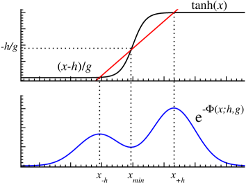
Figure 7: Solutions for the mean field equation (26) with two maxima and one minimum for a positive value of the field $h$.

We define the mean values from the distribution equation (25). If the field $h$ is not zero, as shown in figure 7, $\left[\exp\left(-\Phi\right)\right]^{n}$ develops one dominant maximum as $n\to\infty$. For large enough $n$, only this maximum contributes to the integrals (25) and the algorithm obtained from this assumption turns out to be the same as the one presented in  KabashimaCDMA . However, if the field is sufficiently small it gives rise to a new regime where the two maxima contribute. At the same time, it is important to note that a small, non zero field favours the solution of Eq.(26) that satisfies ${\rm sgn}(x)={\rm sgn}(h).$ To analyse the behaviour of the field, we will explore the solutions of Eq.(26) in the regime $0\lesssim\left|h\right|\ll 1$. With this aim, suppose that the solutions for the Eq.(26) at zero field are $x_{0}=\pm g_{1}\left|m\right|$ where $m\equiv\tanh\left(x_{0}\right)$ and ${\rm sgn}(m)={\rm sgn}(h)$. If the field is sufficiently small one can expand the solutions of equation (26) as $x_{\pm h}=\pm g_{1}m+\xi(m,g_{1})h$ where $\xi(m,g_{1})h$ is expected to be small and satisfies ${\rm sgn}\left(\xi(m,g_{1})h\right)={\rm sgn}(h)$. Observe that if the field is positive (negative), both roots are displaced to the right (left) with respect to the zero field solutions. Using this expression for the roots in Eq.(26) and disregarding terms of $\mathcal{O}\left(h^{2}\right)$ one finds that

$$\xi(m,g_{1})=\frac{1}{1-g_{1}\left(1-m^{2}\right)}\,.$$ (27)

The expression for the exponent $\Phi$ near the roots and in the $0\lesssim\left|h\right|\ll 1$ regime is then $\Phi\left(x_{\pm h};h\to 0,g_{1}\right)\simeq\Phi\left(x_{0};0,g_{1}\right)\mp mh=\Phi_{0}\mp mh\,,$ and, by the definition of the $m$, the product $mh$ is positively defined.

Let us define $\beta_{\pm h}\left(m,g_{1}\right)\equiv\left(1-m^{2}\right)\left[1\mp 2\xi\left(m,g_{1}\right)mh\right]$. We expect that, for large $n$ the following approximation to be valid:

$$\exp\left\{-n\Phi\left(x;h\to 0,g_{1}\right)\right\} \simeq {\rm e}^{-n\Phi_{0}}\left\{{\rm e}^{nmh}\exp\left\{-\frac{n}{2}\left[g_{1}^{-1}-\beta_{h}\left(m,g_{1}\right)\right]\left(x-x_{h}\right)^{2}\right\}\right.$$ (28)

$$\left.\qquad+{\rm e}^{-nmh}\exp\left\{-\frac{n}{2}\left[g_{1}^{-1}-\beta_{-h}\left(m,g_{1}\right)\right]\left(x-x_{-h}\right)^{2}\right\}\right\}\,.$$

Using equation (28) one can calculate the normalisation in equation (24)

$$\mathcal{Z}\left(h\to 0,g_{1}\right) \simeq {\rm e}^{-n\left(\Phi_{0}-mh\right)}\int{\rm d}x\,\exp\left\{-\frac{n}{2}\left[g_{1}^{-1}-\beta_{h}\left(m,g_{1}\right)\right]\left(x-x_{h}\right)^{2}\right\}$$ (29)

$$+{\rm e}^{-n\left(\Phi_{0}+mh\right)}\int{\rm d}x\,\exp\left\{-\frac{n}{2}\left[g_{1}^{-1}-\beta_{-h}\left(m,g_{1}\right)\right]\left(x-x_{-h}\right)^{2}\right\}$$

$$\simeq \sqrt{\frac{2\pi g_{1}\xi\left(m,g_{1}\right)}{n}}\!\,{\rm e}^{-n\Phi_{0}}\!\left\{\,{\rm e}^{nmh}\!\left(1-g_{1}\left(1-m^{2}\right)\xi^{2}\left(m,g_{1}\right)\,mh\right)\right.$$

$$\qquad\qquad\qquad\left.+\,\,{\rm e}^{-nmh}\!\left(1+g_{1}\left(1-m^{2}\right)\xi^{2}\left(m,g_{1}\right)\,mh\right)\right\}\,\,.$$

The mean value of a given function $f(x)$ with respect to the conditional probability distribution defined in equation (25) is then:

$$\left\langle f(x)|h\to 0,g_{1}\right\rangle \simeq \mathcal{Z}^{-1}{\rm e}^{-n\left(\Phi_{0}-mh\right)}\int\!\!{\rm d}x\,\exp\left\{-\frac{n}{2}\left[g_{1}^{-1}\!-\!\left(1\!-\!m^{2}\right)\!\left(1\!-\!2\xi\left(m,g_{1}\right)\,mh\right)\right]\!\left(x\!-\!x_{h}\right)^{2}\right\}$$

$$\qquad\qquad\qquad\qquad\qquad\left[f\left(x_{h}\right)+\left(x-x_{h}\right)f^{\prime}\left(x_{h}\right)+\frac{1}{2}\left(x-x_{h}\right)^{2}f^{\prime\prime}\left(x_{h}\right)\right]$$

$$+\mathcal{Z}^{-1}{\rm e}^{-n\left(\Phi_{0}+mh\right)}\int\!\!{\rm d}x\,\exp\left\{-\frac{n}{2}\left[g_{1}^{-1}\!-\!\left(1\!-\!m^{2}\right)\!\left(1\!+\!2\xi\left(m,g_{1}\right)\,mh\right)\right]\!\left(x\!-\!x_{-h}\right)^{2}\right\}$$

$$\qquad\qquad\qquad\qquad\qquad\left[f\left(x_{-h}\right)+\left(x-x_{-h}\right)f^{\prime}\left(x_{-h}\right)+\frac{1}{2}\left(x-x_{-h}\right)^{2}f^{\prime\prime}\left(x_{-h}\right)\right]\,,$$

which implies, considering that the integrals of the linear terms are zero and keeping only the leading terms in the expansions, that the expectation values takes the form:

$$\left\langle f(x)|h\to 0,g_{1}\right\rangle \simeq \left[1-{\rm e}^{-2nmh}\left(1+2\xi^{2}\left(m,g_{1}\right)\,mh\right)\right]\left\{f\left(x_{h}\right)+\frac{g_{1}}{2n}\xi\left(m,g_{1}\right)\,f^{\prime\prime}\left(x_{h}\right)\right\}$$

$$+{\rm e}^{-2nmh}\left(1+2\xi^{2}\left(m,g_{1}\right)\,mh\right)f\left(x_{-h}\right)\,.$$

Considering the expansion of $f\left(x_{\pm h}\right)\simeq f\left(\pm g_{1}m+\xi\left(m,g_{1}\right)\,h\right)\simeq f\left(\pm g_{1}m\right)+\xi\left(m,g_{1}\right)\,f^{\prime}\left(\pm g_{1}m\right)\,h$ and disregarding terms of $\mathcal{O}\left(h{\rm e}^{-2nmh}\right)$, one can write:

$$\left\langle f(x)|h\!\to\!0,g_{1}\right\rangle\simeq f\left(mg_{1}\right)\!+\!\frac{g_{1}}{2n}\xi\left(m,g_{1}\right)f^{\prime\prime}\left(mg_{1}\right)\!-\!{\rm e}^{-2nmh}\!\left[f\left(mg_{1}\right)\!-\!f\left(\!-\!mg_{1}\right)\right]\!+\!f^{\prime}\left(mg_{1}\right)\!\xi\left(m,g_{1}\right)h.$$ (30)

The resulting one and two variable expectation values become

$$\left\langle b_{k}^{\textrm{a}}|h_{\mu k}^{t}\to 0,g_{\mu k}^{t}\right\rangle = \sum_{\left\{\mathbf{b}_{k}\right\}}P^{t}\left(\mathbf{b}_{k}|\left\{y_{\nu\neq\mu}\right\}\right)b_{k}^{\textrm{a}}=\left\langle\tanh(x)|h_{\mu k}^{t}\to 0,g_{1\mu k}^{t}\right\rangle$$

$$\simeq \left[1-\frac{g_{1\mu k}^{t}}{n}\left[1-\left(m_{\mu k}^{t}\right)^{2}\right]\xi\left(m_{\mu k}^{t},g_{1\mu k}^{t}\right)-2{\rm e}^{-2nm_{\mu k}^{t}h_{\mu k}^{t}}\right]m_{\mu k}^{t}$$

$$\qquad\qquad+\xi\left(m_{\mu k}^{t},g_{1\mu k}^{t}\right)\,\left[1-\left(m_{\mu k}^{t}\right)^{2}\right]h_{\mu k}^{t}$$

and

$$\left\langle b_{k}^{\textrm{a}}b_{k}^{\textrm{b}}|h_{\mu k}^{t}\to 0,g_{1\mu k}^{t}\right\rangle = P^{t}\left(\mathbf{b}_{k}|\left\{y_{\nu\neq\mu}\right\}\right)b_{k}^{\textrm{a}}b_{k}^{\textrm{b}}=\delta^{\textrm{ab}}+\left(1-\delta^{\textrm{ab}}\right)\left\langle\tanh^{2}(x)|h_{\mu k}^{t}\to 0,g_{1\mu k}^{t}\right\rangle\,,$$

where

$$\left\langle\tanh^{2}(x)|h_{\mu k}^{t}\to 0,g_{1\mu k}^{t}\right\rangle=\left(m_{\mu k}^{t}\right)^{2}+\xi\left(m_{\mu k}^{t},g_{1\mu k}^{t}\right)\left[1-\left(m_{\mu k}^{t}\right)^{2}\right]\,\left\{\frac{g_{1\mu k}^{t}}{n}\,\left[1-3\left(m_{\mu k}^{t}\right)^{2}\right]+2m_{\mu k}^{t}h_{\mu k}^{t}\right\}\,,$$

and

$$\left\langle b_{k}^{\textrm{a}}b_{l}^{\textrm{b}}|h_{\mu k}^{t}\to 0,g_{1\mu k}^{t}\right\rangle=\left\langle b_{k}^{\textrm{a}}|h_{\mu k}^{t}\to 0,g_{1\mu k}^{t}\right\rangle\left\langle b_{l}^{\textrm{b}}|h_{\mu k}^{t}\to 0,g_{1\mu k}^{t}\right\rangle.$$

Thus, the leading terms for the covariance matrix of the replicated variables are:

$$\left(\mathbf{{\Psi}}_{\mu kl}^{t}\right)^{\mathrm{ab}} \equiv \left\langle b_{k}^{\textrm{a}}b_{l}^{\textrm{b}}|h_{\mu k}^{t}\to 0,g_{1\mu k}^{t};h_{\mu l}^{t}\to 0,g_{1\mu l}^{t}\right\rangle-\left\langle b_{k}^{\textrm{a}}|h_{\mu k}^{t}\to 0,g_{1\mu k}^{t}\right\rangle\left\langle b_{l}^{\textrm{b}}|h_{\mu l}^{t}\to 0,g_{1\mu l}^{t}\right\rangle=\delta_{kl}\left(\mathbf{{\Psi}}_{\mu k}^{t}\right)^{\mathrm{ab}}$$

$$\left(\mathbf{{\Psi}}_{\mu k}^{t}\right)^{\mathrm{ab}} \simeq \delta^{{\rm ab}}\left[1-\left(m_{\mu k}^{t}\right)^{2}\right]$$

$$+\left(1-\delta^{{\rm ab}}\right)\left\{\frac{g_{1\mu k}^{t}}{n}\xi\left(m_{\mu k}^{t},g_{1\mu k}^{t}\right)\left[1-\left(m_{\mu k}^{t}\right)^{2}\right]^{2}+4{\rm e}^{-2nm_{\mu k}^{t}h_{\mu k}^{t}}\left(1-{\rm e}^{-2nm_{\mu k}^{t}h_{\mu k}^{t}}\right)\left(m_{\mu k}^{t}\right)^{2}\right\}\,.$$

If one requires the non-diagonal elements of this covariance matrix to have the same scaling as the inter-replica interaction matrix, the field has to behave in such a way that the exponential term contributes at most in $\mathcal{O}\left(n^{-1}\right).$ One thus expects the field to obey $m_{\mu k}^{t}h_{\mu k}^{t}<{\displaystyle\frac{1}{n}}\ln\left|{\displaystyle\frac{2n}{n_{\mu k}^{t}}}\right|$, where the $n_{\mu k}^{t}$ are appropriate constants. With this asymptotic behaviour, the expression for the entries in the covariance matrix is

$$\left(\mathbf{{\Psi}}_{\mu k}^{t}\right)^{\mathrm{ab}}\simeq\delta^{{\rm ab}}\left[1-\left(m_{\mu k}^{t}\right)^{2}\right]+\left(1-\delta^{{\rm ab}}\right)\,\frac{g_{1\mu k}^{t}\xi\left(m_{\mu k}^{t},g_{1\mu k}^{t}\right)}{n}\,\left[1-\left(m_{\mu k}^{t}\right)^{2}\right]^{2}\,,$$

which serves to define the probability distribution for the macroscopic variable $\Delta_{\mu k}^{\mathrm{a}}=\sum_{l\neq k}\varepsilon_{\mu l}b_{l}^{\mathrm{a}}$.

As $\varepsilon_{\mu k}$ and $b_{k}^{\mathrm{a}}$ are unbiased variables, the variable $\Delta_{\mu k}^{\mathrm{a}}$, by virtue of the central limit theorem, obeys a normal distribution, with mean value and covariance matrix given by (to highest order)

$$\left(\mathbf{u}_{\mu k}^{t}\right)^{\mathrm{a}}\equiv\left\langle\Delta_{\mu k}^{\mathrm{a}}\right\rangle = \sum_{\left\{\mathbf{b}_{l\neq k}\right\}}\prod_{l\neq k}P^{t}\left(\mathbf{b}_{l}|\left\{y_{\nu\neq\mu}\right\}\right)\sum_{l\neq k}\varepsilon_{\mu l}b_{l}^{\mathrm{a}}=\sum_{l\neq k}\varepsilon_{\mu l}m_{\mu l}^{t}$$ (31)

$$\left(\mathbf{{\Upsilon}}_{\mu k}^{t}\right)^{\mathrm{ab}}\equiv\left\langle\Delta_{\mu k}^{\textrm{a}}\Delta_{\mu k}^{\textrm{b}}\right\rangle-\left\langle\Delta_{k}^{\textrm{a}\phantom{b}}\right\rangle\left\langle\Delta_{k}^{\textrm{b}}\right\rangle = \sum_{\left\{\mathbf{b}_{l\neq k}\right\}}\prod_{l\neq k}P^{t}\left(\mathbf{b}_{l}|\left\{y_{\nu\neq\mu}\right\}\right)\sum_{\begin{subarray}{c}l\neq k\\ j\neq k\end{subarray}}\varepsilon_{\mu l}\varepsilon_{\mu j}b_{l}^{\mathrm{a}}b_{j}^{\mathrm{b}}-\left(\sum_{l\neq k}\varepsilon_{\mu l}m_{\mu l}^{t}\right)^{2}$$

$$= \sum_{l\neq k}\varepsilon_{\mu l}^{2}\left(\mathbf{{\Psi}}_{\mu lj}^{t}\right)^{\mathrm{ab}}=\delta^{\mathrm{ab}}X_{\mu k}+\left(1-\delta^{\mathrm{ab}}\right)\frac{1}{n}R_{\mu k}^{t},$$

where

$$X_{\mu k}^{t} \equiv \sum_{l\neq k}\varepsilon_{\mu l}^{2}\,\left[1-\left(m_{\mu l}^{t}\right)^{2}\right]\mbox{\leavevmode\nobreak\ \leavevmode\nobreak\ \leavevmode\nobreak\ and}$$ (32)

$$R_{\mu k}^{t} \equiv \sum_{l\neq k}\varepsilon_{\mu l}^{2}\,g_{1\mu l}^{t}\,\xi\left(m_{\mu l}^{t},g_{1\mu l}^{t}\right)\left[1-\left(m_{\mu l}^{t}\right)^{2}\right]^{2}\,,$$

are macroscopic variables of $\mathcal{O}(1)$. In particular, $R_{\mu k}^{t}$ is a free variable that can be used later on to optimise a given performance measure. This variables have the property of being self-averaging, therefore we can drop the sub-indices $\mu$ and k.

Appendix B The One Step Replica Symmetry Breaking (1RSB) Ansatz

Under a solution correlation matrix that resembles the 1RSB structure, the system comprises $nL$ variables, where both the number of blocks L and the number of variables per block n are considered large. As before we are interested in the regime where $L$ and $n\to\infty.$

With this setting, the interaction term in equation (6) is now:

$$\mathbf{b}_{k}^{\sf T}\mathbf{Q}_{\mu k}^{t}\mathbf{b}_{k}=-q_{1\mu k}^{t}nL+\left(q_{1\mu k}^{t}-q_{2\mu k}^{t}\right)\sum_{\ell=1}^{L}\left(\sum_{{\rm a}=1}^{n}b_{k}^{\ell{\rm a}}\right)^{2}+q_{2\mu k}^{t}\left(\sum_{\ell=1}^{L}\sum_{{\rm a}=1}^{n}b_{k}^{\ell{\rm a}}\right)^{2}\,,$$

thus we have now $L+1$ squared sums in the exponent that can be replaced by integrals:

$$P^{t}\left(\mathbf{b}_{k}|\left\{y_{\nu\neq\mu}\right\}\right) = [\mathcal{Z}_{\mu k}^{t}]^{-1}{\displaystyle\int\mathrm{d}\mathbold{x}}\,\exp\left\{-\frac{x_{0}^{2}}{2q_{2\mu k}^{t}}-\sum_{\ell=1}^{L}\frac{x_{\ell}^{2}}{2\upDelta q_{\mu k}^{t}}+\sum_{\ell=1}^{L}\left(x_{0}+x_{\ell}+h_{\mu k}^{t}\right)\sum_{\mathrm{a}=1}^{n}b_{k}^{\ell\mathrm{a}}\right\}\,,$$

where $\upDelta q_{\mu k}^{t}\equiv q_{1\mu k}^{t}-q_{2\mu k}^{t}>0$ and $\mathbold x^{\sf T}=\left(x_{0},x_{1},\dots,x_{L}\right)$. Also here we expect the logarithm of the normalisation term (linked to the free energy) obtained from the well behaved distribution $P^{t}$ to be self-averaging, thus:

$$\lim_{n\to\infty}\lim_{L\to\infty}\frac{1}{nL}\log\left(\overline{\mathcal{Z}_{\mu k}^{t}}\right)=\lim_{n\to\infty}\lim_{L\to\infty}\frac{1}{nL}\log\left(\mathcal{Z}_{\mu k}^{t}\left(h_{\mu k}^{t},q_{1\mu k}^{t},q_{2\mu k}^{t}\right)\right),$$

which is satisfied if the entries behave like $q_{2\mu k}^{t}\sim g_{2\mu k}^{t}/nL$ and $\upDelta q_{\mu k}^{t}\sim g_{1\mu k}^{t}/n,$ where $g_{1\mu k}^{t}$ and $g_{2\mu k}^{t}\sim\mathcal{O}(1)$. Using this new scaled parameters, the expression for the normalisation is $\mathcal{Z}_{\mu k}^{t}=\int{\rm d}\mathbf{x}\,\exp\left\{-nL\Phi\left(\mathbf{x};h_{\mu k}^{t},g_{1\mu k}^{t},g_{2\mu k}^{t}\right)\right\}$ where

$$\Phi\left(\mathbf{x};h_{\mu k}^{t},g_{1\mu k}^{t},g_{2\mu k}^{t}\right)\equiv\frac{x_{0}^{2}}{2g_{1\mu k}^{t}}+\frac{1}{L}\sum_{\ell=1}^{L}\frac{x_{\ell}^{2}}{2g_{2\mu k}^{t}}-\frac{1}{L}\sum_{\ell=1}^{L}\log\left[2\cosh\left(x_{0}+x_{\ell}+h_{\mu k}^{t}\right)\right]\,.$$

As before, we drop the indexes $\mu$, k, and t for brevity. The critical points of the function $\Phi\left(\mathbf{x};h,g_{1},g_{2}\right)$ satisfy the following set of equations:

$$\frac{\partial\Phi}{\partial x_{0}} = \frac{x_{0}}{g_{1}}-\frac{1}{L}\sum_{\ell=1}^{L}\tanh\left(x_{0}+x_{\ell}+h\right)=0$$

$$\frac{\partial\Phi}{\partial x_{\ell}} = \frac{1}{L}\left(\frac{x_{\ell}}{g_{2}}-\tanh\left(x_{0}+x_{\ell}+h\right)\right)=0\,,$$

which are satisfied for the following values:

$$x_{0}^{*} = \frac{g_{1}}{g_{2}}\,\frac{1}{L}\sum_{\ell=1}^{L}x_{\ell}^{*}=\frac{g_{1}}{g_{2}}x^{*}$$

$$\frac{x_{\ell}^{*}}{g_{2}} = \tanh\left(x_{\ell}^{*}+\frac{g_{1}}{g_{2}}x^{*}+h\right)\,,$$ (33)

where $x^{*}\equiv\frac{1}{L}\sum_{\ell=1}^{L}x_{\ell}^{*}$. The second equation in the set, equation (33), has the same form for all $\ell=1,\dots,L$ and in the small field regime it has at most three different solutions. From the three possible solutions, one is a local maximum; of the other two, the one that has the same sign as h is dominant. Thus we can expect, for all $\ell$, $x_{\ell}^{*}=x^{*}$. This reduces the set of $L+1$ equations to one

$$\frac{x^{*}}{g_{2}}=\tanh\left(\frac{G}{g_{2}}x^{*}+h\right)\,,$$

where $G\equiv g_{1}+g_{2}$. With the substitution $u=\left(G/g_{2}\right)x^{*}$ the equation has the same form as equation (26), i.e. $u=G\,\tanh\left(u+h\right).$ If one considers again the field h to be small, the solutions can be expressed as an expansion of the zero field solutions $u_{\pm h}\simeq\pm Gm+\xi(m,G)h$, where $\xi(m,G)$ is given by equation (27), and ${\rm sgn}(m)={\rm sgn}(h).$ Using these expansions the critical values are given by: $x_{0,\pm h}^{*}\simeq g_{1}\left[\pm m+G^{-1}\xi(m,G)h\right]$ and $x_{\ell,\pm h}^{*}\simeq g_{2}\left[\pm m+G^{-1}\xi(m,G)h\right]$ for all $\ell=1,\dots,L.$

As in the RS case, the expansion of $\Phi$ around the critical points in the small field regime is $\Phi\left(\mathbf{x}_{\pm h}^{*};h\to 0,g_{1},g_{2}\right)\simeq\Phi\left(\mathbf{x}_{0}^{*};0,g_{1},g_{2}\right)\mp mh=\Phi_{0}\mp mh$. So the dominant solution is the one that shares the sign with the field.

For a sufficiently large system with $nL$ variables, one expects the following expansion to be valid:

$$\exp\left\{-nL\Phi\left(\mathbf{x};h\to 0,g_{1},g_{2}\right)\right\} \simeq {\rm e}^{-nL\Phi_{0}}\left\{{\rm e}^{nLmh}\exp\left[-\frac{nL}{2}\left(\mathbf{x}-\mathbf{x}_{h}^{*}\right)^{\sf T}\mathbf{H}_{\Phi,h}\left(\mathbf{x}-\mathbf{x}_{h}^{*}\right)\right]\right.$$ (34)

$$\left.\qquad\quad+{\rm e}^{-nLmh}\exp\left[-\frac{nL}{2}\left(\mathbf{x}\!-\!\mathbf{x}_{-h}^{*}\right)^{\sf T}\mathbf{H}_{\Phi,-h}\left(\mathbf{x}\!-\!\mathbf{x}_{-h}^{*}\right)\right]\right\}\,,$$

where $\mathbf{H}_{\Phi,\pm h}$ is the Hessian of $\Phi$ in $\mathbf{x}_{\pm h}^{*}$.

Defining $\beta_{\pm h}\equiv\left(1-m^{2}\right)\left\{1\mp 2\left[\xi(m,G)+1\right]\,mh\right\}$, the entries of the Hessian become

$$\left.\frac{\partial^{2}\Phi}{\partial x_{0}^{2}}\right|_{\mathbf{x}_{\pm h}^{*}} \simeq g_{1}^{-1}-\beta_{\pm h}\equiv\alpha_{\pm h}$$

$$\left.\frac{\partial^{2}\Phi}{\partial x_{\ell}^{2}}\right|_{\mathbf{x}_{\pm h}^{*}} \simeq \frac{1}{L}\left(g_{2}^{-1}-\beta_{\pm h}\right)\equiv\frac{1}{L}\gamma_{\pm h}$$

$$\left.\frac{\partial^{2}\Phi}{\partial x_{0}\partial x_{\ell}}\right|_{\mathbf{x}_{\pm h}^{*}} \simeq -\frac{1}{L}\beta_{\pm h}$$

$$\left.\frac{\partial^{2}\Phi}{\partial x_{\ell}\partial x_{\ell^{\prime}}}\right|_{\mathbf{x}_{\pm h}^{*}} = 0\leavevmode\nobreak\ .$$

The corresponding characteristic equation is:

$$\det\left(\mathbf{H}_{\Phi,\pm h}-\lambda\openone\right)=\left(\frac{1}{L}\gamma_{\pm h}-\lambda\right)^{L-1}\left\{\left(\alpha_{\pm h}-\lambda\right)\left(\frac{1}{L}\gamma_{\pm h}-\lambda\right)-\frac{1}{L}\beta_{\pm h}^{2}\right\}=0\,.$$

The solutions for this equation, disregarding terms of $\mathcal{O}\left(L^{-2}\right)$ and $\mathcal{O}\left(hL^{-1}\right)$, are:

$$\lambda_{0,\pm h} = \alpha_{\pm h}+\frac{1}{L}\frac{\beta_{\pm h}^{2}}{\alpha_{\pm h}}$$

$$\simeq \lambda_{0}\left\{1\pm 2\left[\xi(m,g_{1})-1\right]\left[\xi(m,G)+1\right]\left(1-m^{2}\right)\,mh\right\}$$

$$\lambda_{1,\pm h} = \frac{1}{L}\left(\gamma_{\pm h}-\frac{\beta_{\pm h}^{2}}{\alpha_{\pm h}}\right)$$

$$\simeq \lambda_{1}\left\{1\pm 2\frac{\xi(m,g_{1})^{2}\left[\xi(m,g_{2})-1\right]}{1-\left[\xi(m,g_{1})-1\right]\left[\xi(m,g_{2})-1\right]}\left[\xi(m,G)+1\right]\left(1-m^{2}\right)\,mh\right\}$$

$$\lambda_{\ell,\pm h} = \frac{1}{L}\gamma_{\pm h}$$

$$\simeq \lambda_{\ell}\left\{1\pm 2\left[\xi(m,g_{2})-1\right]\left[\xi(m,G)+1\right]\left(1-m^{2}\right)\,mh\right\}\quad\forall\,\ell=2,\dots,L\,,$$

where $\lambda_{0}\equiv\alpha_{0}+\frac{1}{L}\,\frac{\beta_{0}^{2}}{\alpha_{0}}$, $\lambda_{1}\equiv\frac{1}{L}\left(\gamma_{0}-\frac{\beta_{0}^{2}}{\alpha_{0}}\right)$ and $\lambda_{\ell}\equiv\frac{1}{L}\gamma_{0}$. The corresponding eigenvectors, up to order $L^{-1}$, are:

$$\mathbf{u}_{0,\pm h} = \left(1,\stackrel{{\scriptstyle L\;{\rm times}}}{{\overbrace{-\frac{1}{L}\,\frac{\beta_{\pm h}}{\alpha_{\pm h}},-\frac{1}{L}\,\frac{\beta_{\pm h}}{\alpha_{\pm h}},\dots,-\frac{1}{L}\,\frac{\beta_{\pm h}}{\alpha_{\pm h}}}}}\right)^{\sf T}$$

$$\mathbf{u}_{1,\pm h} = \frac{1}{\sqrt{L}}\left(\frac{\beta_{\pm h}}{\alpha_{\pm h}},\stackrel{{\scriptstyle L\;{\rm times}}}{{\overbrace{1,1,\dots,1}}}\right)^{\sf T}$$ (36)

$$\mathbf{u}_{\ell,\pm h} = \frac{1}{\sqrt{\ell\left(\ell-1\right)}}\left(0,\stackrel{{\scriptstyle\ell-1\;{\rm times}}}{{\overbrace{1,1,\dots,1}}},-\left(\ell-1\right),\stackrel{{\scriptstyle L-\ell\;{\rm times}}}{{\overbrace{0,0,\dots,0}}}\right)^{\sf T}\quad\forall\,\ell=2,\dots,L\,.$$

These vectors satisfy the normalisation condition $\mathbf{u}_{\ell,\pm h}^{\sf T}\mathbf{u}_{\ell^{\prime},\pm h}=\delta^{\ell\ell^{\prime}}\left[1+\mathcal{O}\left(L^{-1}\right)\right]\;\;\forall\ell,\ell^{\prime}=0,1,\dots,L.$ The linear transformation from the canonical basis to the basis of eigenvectors is then represented by a matrix with the entries

$$\left(\mathbf{U}_{\pm h}\right)_{ij}\simeq\left(\mathbf{U}_{0}\right)_{ij} = \delta_{0i}\delta_{0j}+\frac{1}{\sqrt{j(j-1)}}\left[\sum_{k=1}^{j-1}\delta_{ki}-\left(1-\delta_{0j}\right)\left(1-\delta_{1j}\right)\delta_{ij}(j-1)\right]$$ (37)

$$+\frac{1}{\sqrt{L}}\,\delta_{1j}\left[\delta_{0i}\,\frac{\beta_{0}}{\alpha_{0}}+\left(1-\delta_{0i}\right)\right]-\frac{1}{L}\,\delta_{0j}\left(1-\delta_{0i}\right)\,\frac{\beta_{0}}{\alpha_{0}}\,,$$

ignoring terms of $\mathcal{O}\left(hL^{-1/2}\right)$. Because this transformation is a rigid rotation, the following properties are satisfied: $\left|\det\left(\mathbf{U}_{\pm}\right)\right|=1$ and $\mathbf{U}_{\pm h}^{\sf T}\mathbf{U}_{\pm h}=\mathbf{U}_{\pm h}\mathbf{U}_{\pm h}^{\sf T}=\openone.$

Second order terms in equation (34) can be re-written using the diagonal representation of the Hessian. Therefore, keeping only terms of order $\mathcal{O}\left(L^{-1}\right)$ we have that: $\left(\mathbf{x}-\mathbf{x}_{\pm h}\right)^{\sf T}\mathbf{H}_{\Phi,\pm h}\left(\mathbf{x}-\mathbf{x}_{\pm h}\right)=\left(\mathbf{x}-\mathbf{x}_{\pm h}\right)^{\sf T}\mathbf{U}_{0}\mathbf{U}_{0}^{\sf T}\mathbf{H}_{\Phi,\pm h}\mathbf{U}_{0}\mathbf{U}_{0}^{\sf T}\left(\mathbf{x}-\mathbf{x}_{\pm h}\right)=\left(\mathbf{y}-\mathbf{y}_{\pm h}\right)^{\sf T}\mathbf{H}_{\Phi,\pm h}^{\prime}\left(\mathbf{y}-\mathbf{y}_{\pm h}\right)$, where $\mathbf{y}\equiv\mathbf{U}_{0}^{\sf T}\mathbf{x}$ and $\mathbf{H}_{\Phi,\pm h}^{\prime}\equiv\mathbf{U}_{0}^{\sf T}\mathbf{H}_{\Phi,\pm h}\mathbf{U}_{0}$ is the diagonal representation of the Hessian, i.e. $\left(\mathbf{H}_{\Phi,\pm h}^{\prime}\right)_{ij}=\delta_{ij}\lambda_{i,\pm h}$. Using the diagonal representation in conjunction with equation (34) one obtains an expression for the normalisation term

$$\mathcal{Z}\left(h\to 0,g_{1},g_{2}\right) \simeq {\rm e}^{-nL\left(\Phi_{0}-mh\right)}\int{\rm d}\mathbf{y}\,\exp\left[-\frac{nL}{2}\left(\mathbf{y}-\mathbf{y}_{h}^{*}\right)^{\sf T}\mathbf{H}_{\Phi,h}^{\prime}\left(\mathbf{y}-\mathbf{y}_{h}^{*}\right)\right]$$

$$+{\rm e}^{-nL\left(\Phi_{0}+mh\right)}\int{\rm d}\mathbf{y}\,\exp\left[-\frac{nL}{2}\left(\mathbf{y}-\mathbf{y}_{-h}^{*}\right)^{\sf T}\mathbf{H}_{\Phi,-h}^{\prime}\left(\mathbf{y}-\mathbf{y}_{-h}^{*}\right)\right]$$

$$\simeq {\rm e}^{-nL\Phi_{0}}\left(\frac{2\pi}{nL}\right)^{\frac{L+1}{2}}\left[{\rm e}^{nLmh}\prod_{\ell=0}^{L}\lambda_{\ell,h}^{-\frac{1}{2}}+{\rm e}^{-nLmh}\prod_{\ell=0}^{L}\lambda_{\ell,-h}^{-\frac{1}{2}}\right]\,.$$

For a small field, the product of the eigenvalues can be approximated by

$$\prod_{\ell=0}^{L}\lambda_{\ell,\pm h}^{-\frac{1}{2}} \simeq \left\{1\mp\left[\xi(m,g_{2})-1\right]\left[\xi(m,G)+1\right]Lmh\right\}\prod_{\ell=0}^{L}\lambda_{\ell}^{-\frac{1}{2}}\,.$$

Thus, the expression for $\mathcal{Z}$ reduces to

$$\mathcal{Z}\left(h\to 0,g_{1},g_{2}\right) \simeq {\rm e}^{-nL\Phi_{0}}\left(\frac{2\pi}{nL}\right)^{\frac{L+1}{2}}\prod_{\ell=0}^{L}\lambda_{\ell}^{-\frac{1}{2}}\left\{{\rm e}^{nLmh}\left\{1-\left[\xi(m,g_{2})-1\right]\left[\xi(m,G)+1\right]Lmh\right\}\right.$$

$$\qquad\qquad\qquad+\left.{\rm e}^{-nLmh}\left\{1+\left[\xi(m,g_{2})-1\right]\left[\xi(m,G)+1\right]Lmh\right\}\right\}\,.$$

The mean value of a given function $f(\mathbf{x})$ is then given by

$$\left\langle f(\mathbf{x})|h\to 0,g_{1},g_{2}\right\rangle \simeq \mathcal{Z}^{-1}{\rm e}^{-nL\left(\Phi_{0}-mh\right)}\int{\rm d}\mathbf{y}\,\exp\left\{-\frac{nL}{2}\left(\mathbf{y}-\mathbf{y}_{h}^{*}\right)^{\sf T}\mathbf{H}_{\Phi,h}^{\prime}\left(\mathbf{y}-\mathbf{y}_{h}^{*}\right)\right\}$$

$$\qquad\qquad\qquad\qquad\qquad\left[f\left(\mathbf{x}_{h}\right)+\frac{1}{2}\left(\mathbf{y}-\mathbf{y}_{h}^{*}\right)^{\sf T}\mathbf{H}_{f,h}^{\prime}\left(\mathbf{y}-\mathbf{y}_{h}^{*}\right)\right]$$

$$+\mathcal{Z}^{-1}{\rm e}^{-nL\left(\Phi_{0}+mh\right)}\int{\rm d}\mathbf{y}\,\exp\left\{-\frac{nL}{2}\left(\mathbf{y}-\mathbf{y}_{-h}^{*}\right)^{\sf T}\mathbf{H}_{\Phi,-h}^{\prime}\left(\mathbf{y}-\mathbf{y}_{-h}^{*}\right)\right\}$$

$$\qquad\qquad\qquad\qquad\qquad\left[f\left(\mathbf{x}_{-h}\right)+\frac{1}{2}\left(\mathbf{y}-\mathbf{y}_{-h}^{*}\right)^{\sf T}\mathbf{H}_{f,-h}^{\prime}\left(\mathbf{y}-\mathbf{y}_{-h}^{*}\right)\right]\,,$$

where $\mathbf{H}_{f,\pm h}^{\prime}$ is the Hessian of the function $f$ in the basis of eigenvectors of $\mathbf{H}_{\Phi\pm h}$, evaluated at the critical points. The linear terms in the expansion of $f\left(\mathbf{x}\right)$ do not contribute to the expectation value. The Gaussian integral of the cross products of the type $\left(y_{i}-y_{i,\pm h}^{*}\right)\left(y_{j}-y_{j,\pm h}^{*}\right)$ with $i\neq j$ are zero, thus the Gaussian integral of the second term in the expansion of $f\left(\mathbf{x}\right)$ becomes:

$$I_{\pm} = \frac{1}{2}\mathcal{Z}^{-1}{\rm e}^{-nL\left(\Phi_{0}\mp mh\right)}\int{\rm d}\mathbf{y}\,\exp\left[-\frac{nL}{2}\left(\mathbf{y}-\mathbf{y}_{\pm h}^{*}\right)^{\sf T}\mathbf{H}_{\Phi,\pm h}^{\prime}\left(\mathbf{y}-\mathbf{y}_{\pm h}^{*}\right)\right]\left(\mathbf{y}-\mathbf{y}_{\pm h}^{*}\right)^{\sf T}\mathbf{H}_{f,\pm h}^{\prime}\left(\mathbf{y}-\mathbf{y}_{\pm h}^{*}\right)$$

$$I_{+} \simeq \frac{1}{2}\,\left\{1-{\rm e}^{-2nLmh}\left\{1+2\left[\xi(m,g_{2})-1\right]\left[\xi(m,G)+1\right]Lmh\right\}\right\}\;\frac{1}{nL}\,\sum_{\ell=0}^{L}\lambda_{\ell,h}^{-1}\left(\mathbf{H}_{f,h}^{\prime}\right)_{\ell\ell}$$

$$I_{-} \simeq \frac{1}{2}\,{\rm e}^{-2nLmh}\left\{1+2\left[\xi(m,g_{2})-1\right]\left[\xi(m,G)+1\right]Lmh\right\}\;\frac{1}{nL}\,\sum_{\ell=0}^{L}\lambda_{\ell,-h}^{-1}\left(\mathbf{H}_{f,-h}^{\prime}\right)_{\ell\ell}\,.$$ (38)

Using the expansion $f\left(\mathbf{x_{\pm}}\right)\simeq f\left(\pm\mathbf{x}_{0}+h\,\mathbold{\xi}(m,G)\right)\simeq f\left(\pm\mathbf{x}_{0}\right)+h\,\mathbold\xi^{\sf T}(m,G)\nabla f\left(\pm\mathbf{x}_{0}\right)=f\left(\pm\mathbf{x}_{0}\right)+\delta f\left(\pm\mathbf{x}_{0}\right)\,h$ where $\mathbf{x}_{0}^{\sf T}=m\left(g_{1},\stackrel{{\scriptstyle L\;{\rm times}}}{{\overbrace{g_{2},g_{2},\dots,g_{2}}}}\right)$ and $\mathbold\xi^{\sf T}(m,G)=G^{-1}\xi(m,G)\left(g_{1},\stackrel{{\scriptstyle L\;{\rm times}}}{{\overbrace{g_{2},g_{2},\dots,g_{2}}}}\right)$, the diagonal entries of the transformed Hessian are:

$$\left(\mathbf{H}_{f,\pm h}^{\prime}\right)_{\ell\ell} = \sum_{i,j=0}^{L}\left(\mathbf{U}_{\pm h}\right)_{\ell i}\left(\mathbf{U}_{\pm h}\right)_{\ell j}\left(\mathbf{H}_{f,\pm h}\right)_{ij}$$

$$= \sum_{i,j=0}^{L}\left(\mathbf{U}_{\pm h}\right)_{\ell i}\left(\mathbf{U}_{\pm h}\right)_{\ell j}\,\left.\frac{\partial^{2}f}{\partial x_{i}\partial x_{j}}\right|_{\mathbf{x}_{\pm}}$$

$$\simeq \sum_{i,j=0}^{L}\left(\mathbf{U}_{0}\right)_{\ell i}\left(\mathbf{U}_{0}\right)_{\ell j}\,\left(\left.\frac{\partial^{2}f}{\partial x_{i}\partial x_{j}}\right|_{\pm\mathbf{x}_{0}}+h\left.\mathbold\xi^{\sf T}(m,G)\nabla\frac{\partial^{2}f}{\partial x_{i}\partial x_{j}}\right|_{\pm\mathbf{x}_{0}}\right)$$

$$\simeq \left(\left.\mathbf{H}_{f}^{\prime}\right|_{\pm\mathbf{x}_{0}}\right)_{\ell\ell}+\left(\left.\delta\mathbf{H}_{f}^{\prime}\right|_{\pm\mathbf{x}_{0}}\right)_{\ell\ell}h\,,$$

with $\left(\left.\delta\mathbf{H}_{f}^{\prime}\right|_{\pm\mathbf{x}_{0}}\right)_{\ell\ell}$ defined by the second term in (B). Using the entries of the diagonalised Hessian, the last term in the integrals (38) becomes

$$\frac{1}{nL}\,\sum_{\ell=0}^{L}\lambda_{\ell,-h}^{-1}\left(\mathbf{H}_{f,\pm h}^{\prime}\right)_{\ell\ell} \simeq \frac{1}{nL}\,\frac{1}{\alpha_{0}}\,\left(\left.\mathbf{H}_{f}^{\prime}\right|_{\pm\mathbf{x}_{0}}\right)_{00}+\frac{1}{n}\,\frac{\alpha_{0}}{\left(\alpha_{0}\gamma_{0}-\beta_{0}^{2}\right)}\,\left(\left.\mathbf{H}_{f}^{\prime}\right|_{\pm\mathbf{x}_{0}}\right)_{11}+\frac{1}{n}\,\frac{1}{\gamma_{0}}\,\sum_{\ell=2}^{L}\left(\left.\mathbf{H}_{f}^{\prime}\right|_{\pm\mathbf{x}_{0}}\right)_{\ell\ell}\,,$$

disregarding terms of $\mathcal{O}\left(\frac{h}{n}+\frac{h}{L}\right).$ The expectation value of an arbitrary function $f$ can then be approximated by

$$\left\langle f(\mathbf{x})|h\!\to\!0^{+},g_{1},g_{2}\right\rangle \simeq\! f\left(\mathbf{x}_{0}\right)\!+\!\frac{1}{2}\frac{1}{nL}\sum_{\ell=0}^{L}\lambda_{\ell}^{-1}\left(\left.\mathbf{H}_{f}^{\prime}\right|_{\mathbf{x}_{0}}\right)_{\ell\ell}\!-\!{\rm e}^{-2nLmh}\!\left[f\left(\mathbf{x}_{0}\right)\!-\!f\left(-\!\mathbf{x}_{0}\right)\right]\!+\!\delta\!f\!\left(\mathbf{x}_{0}\right)\!h,$$ (40)

where we have disregarded terms of $\mathcal{O}\left(\frac{h}{n}+\frac{h}{L}\right)$,$\mathcal{O}\left(\frac{1}{n}{\rm e}^{-2nLmh}\right)$ and $\mathcal{O}\left(Lh{\rm e}^{-2nLmh}\right)$. By simple inspection, equation (40) is equivalent to the RS mean value equation (30).

The single variable mean value is then:

$$\left\langle b_{k}^{\ell\textrm{a}}|h_{\mu k}^{t}\to 0,g_{1\mu k}^{t},g_{2\mu k}^{t}\right\rangle = {\displaystyle\sum_{\left\{\mathbf{b}_{k}\right\}}}P^{t}\left(\mathbf{b}_{k}|\left\{y_{\nu\neq\mu}\right\}\right)b_{k}^{\ell\textrm{a}}=\left\langle\tanh\left(x_{0}+x_{\ell}+h_{\mu k}^{t}\right)|h_{\mu k}^{t}\to 0,g_{1\mu k}^{t},g_{2\mu k}^{t}\right\rangle\,.$$

The expansion for $f(\mathbf{x})=\tanh\left(x_{0}+x_{\ell}+h_{\mu k}^{t}\right)$ is

$$f(\mathbf{x})\simeq m_{\mu k}^{t}+\left[1-\left(m_{\mu k}^{t}\right)^{2}\right]\left(1,\stackrel{{\scriptstyle\ell-1\;{\rm times}}}{{\overbrace{0,0,\dots,0}}},1,\stackrel{{\scriptstyle L-\ell\;{\rm times}}}{{\overbrace{0,0,\dots,0}}}\right)^{\sf T}\mathbold{\xi}\left(m_{\mu k}^{t},G_{\mu k}^{t}\right)h_{\mu k}^{t}\,,$$

which results in the following expression for the single variable mean value

$$\left\langle b_{k}^{\ell\textrm{a}}|h_{\mu k}^{t}\to 0,g_{1\mu k}^{t},g_{2\mu k}^{t}\right\rangle \simeq \left(1-2{\rm e}^{-2nLm_{\mu k}^{t}h_{\mu k}^{t}}\right)m_{\mu k}^{t}+\xi\left(m_{\mu k}^{t},G_{\mu k}^{t}\right)\,\left[1-\left(m_{\mu k}^{t}\right)^{2}\right]h_{\mu k}^{t}$$

$$-m_{\mu k}^{t}\left[1-\left(m_{\mu k}^{t}\right)^{2}\right]\frac{1}{nL}\sum_{k=0}^{L}\lambda_{k}^{-1}\left(\mathbf{M^{\prime}}_{0\ell}\right)_{kk}\,,$$

where $\left(\mathbf{M}_{0\ell}\right)_{ij}=\delta_{0i}\delta_{0j}+\delta_{0i}\delta_{\ell j}+\delta_{\ell i}\delta_{0j}+\delta_{\ell i}\delta_{\ell j}$ is a matrix such that $\left.\mathbf{H}_{\tanh\left(x_{0}+x_{\ell}\right)}\right|_{\mathbf{x}_{0}}=-2m_{\mu k}^{t}\left[1-\left(m_{\mu k}^{t}\right)^{2}\right]\mathbf{M}_{0\ell}$. In the basis of the $\mathbf{H}_{\Phi}$ eigenvalues, the expressions for the diagonal elements of this matrix are

$$\left(\mathbf{M}_{0\ell}^{\prime}\right)_{kk} = \sum_{i,j=0}^{L}\left(\mathbf{U}_{\pm h}\right)_{ik}\left(\mathbf{U}_{\pm h}\right)_{jk}\left(\delta_{0i}\delta_{0j}+\delta_{0i}\delta_{\ell j}+\delta_{\ell i}\delta_{0j}+\delta_{\ell i}\delta_{\ell j}\right)$$

$$= \left(\left(\mathbf{U}_{\pm h}\right)_{0k}+\left(\mathbf{U}_{\pm h}\right)_{\ell k}\right)^{2}$$

$$\left(\mathbf{M}_{0\ell}^{\prime}\right)_{00} \simeq 1-\frac{2}{L}\,\frac{\beta_{0}}{\alpha_{0}}$$ (41)

$$\left(\mathbf{M}_{0\ell}^{\prime}\right)_{11} \simeq \frac{1}{L}\,\left(\frac{\alpha_{0}+\beta_{0}}{\alpha_{0}}\right)^{2}$$

$$\left(\mathbf{M}_{0\ell}^{\prime}\right)_{kk} = \delta_{k\ell}{\displaystyle\frac{\ell-1}{\ell}}+\Theta\left(k-\ell-1\right)\frac{1}{k\left(k-1\right)}\quad\forall\;\ell=2,\dots,L\,,$$

where $\Theta(n)=1$ if $n>0$ and 0 otherwise. The sum of the eigenvalues’ inverse times the diagonal elements equation (41) results in

$$\frac{1}{nL}\,\sum_{k=0}^{L}\lambda_{k}^{-1}\left(\mathbf{M}_{0\ell}^{\prime}\right)_{kk} \simeq \frac{1}{n}\,\frac{1}{\gamma_{0}}\,\sum_{k=2}^{L}\left[\delta_{k\ell}{\displaystyle\frac{\ell-1}{\ell}}+\Theta\left(k-\ell-1\right)\frac{1}{k\left(k-1\right)}\right]+\frac{1}{nL}\,\frac{1}{\alpha_{0}}\left[1+\frac{\left(\alpha_{0}+\beta_{0}\right)^{2}}{\alpha_{0}\gamma_{0}-\beta_{0}^{2}}\right]$$

$$= \frac{1}{n}\,\frac{1}{\gamma_{0}}\,\left[\sum_{k=2}^{L}\frac{1}{k\left(k-1\right)}\right]+\frac{1}{nL}\,\frac{1}{\alpha_{0}}\left[1+\frac{\left(\alpha_{0}+\beta_{0}\right)^{2}}{\alpha_{0}\gamma-\beta_{0}^{2}}\right]$$

$$= \frac{1}{n}\,\frac{1}{\gamma_{0}}+\frac{1}{nL}\,\frac{1}{\alpha_{0}}\left[1+\frac{\left(\alpha_{0}+\beta_{0}\right)^{2}}{\alpha_{0}\gamma_{0}-\beta_{0}^{2}}-\frac{\alpha_{0}}{\gamma_{0}}\right]$$

$$= \frac{1}{n}\,g_{2\mu k}^{t}\xi\left(m_{\mu k}^{t},g_{2\mu k}^{t}\right)+\frac{1}{nL}\,\left[G_{\mu k}^{t}\xi\left(m_{\mu k}^{t},G_{\mu k}^{t}\right)-g_{2\mu k}^{t}\xi\left(m_{\mu k}^{t},g_{2\mu k}^{t}\right)\right]$$

where we have used that $\sum_{k=2}^{L}\left[k\left(k-1\right)\right]^{-1}=(L-1)/L,$ $\gamma_{0}^{-1}=g_{2\mu k}^{t}\xi\left(m_{\mu k}^{t},g_{2\mu k}^{t}\right)$ and ${\displaystyle\frac{1}{\alpha_{0}}}\left[1+{\displaystyle\frac{\left(\alpha_{0}+\beta_{0}\right)^{2}}{\alpha_{0}\gamma_{0}-\beta_{0}^{2}}}-{\displaystyle\frac{\alpha_{0}}{\gamma_{0}}}\right]=G_{\mu k}^{t}\xi\left(m_{\mu k}^{t},G_{\mu k}^{t}\right)-g_{2\mu k}^{t}\xi\left(m_{\mu k}^{t},g_{2\mu k}^{t}\right).$ The final expression for the expectation value of a single variable is

$$\left\langle b_{k}^{\ell\textrm{a}}|h_{\mu k}^{t}\to 0,g_{1\mu k}^{t},g_{2\mu k}^{t}\right\rangle \simeq \left(1-2{\rm e}^{-2nm_{\mu k}^{t}h_{\mu k}^{t}}\right)m_{\mu k}^{t}-\frac{g_{2\mu k}^{t}\xi\left(m_{\mu k}^{t},g_{2\mu k}^{t}\right)}{n}\left[1-\left(m_{\mu k}^{t}\right)^{2}\right]\,m_{\mu k}^{t}$$ (42)

$$-\frac{G_{\mu k}^{t}\xi\left(m_{\mu k}^{t},G_{\mu k}^{t}\right)-g_{2\mu k}^{t}\xi\left(m_{\mu k}^{t},g_{2\mu k}^{t}\right)}{nL}\left[1-\left(m_{\mu k}^{t}\right)^{2}\right]\,m_{\mu k}^{t}$$

$$+\xi\left(m_{\mu k}^{t},G_{\mu k}^{t}\right)\left[1-\left(m_{\mu k}^{t}\right)^{2}\right]\,h_{\mu k}^{t}\,.$$

To calculate $\left\langle b_{k}^{\ell\textrm{a}}b_{k}^{\ell{\rm a}^{\prime}}|h_{\mu k}^{t}\to 0,g_{\mu k}^{t},\Delta g_{\mu k}^{t}\right\rangle$, an off-diagonal element ($\textrm{a}\neq\textrm{a}^{\prime}$) in the same block $\ell$, we can apply the equation (40) with $f(\mathbf{x})=\tanh^{2}\left(x_{0}+x_{\ell}+h_{\mu k}^{t}\right)$, thus the Hessian matrix is $\left.\mathbf{H}_{\tanh^{2}\left(x_{0}+x_{\ell}\right)}\right|_{\mathbf{x}_{0}}=2\left[1-\left(m_{\mu k}^{t}\right)^{2}\right]\left[1-3\left(m_{\mu k}^{t}\right)^{2}\right]\mathbf{M}_{0\ell}$, thus:

$$\left\langle b_{k}^{\ell\textrm{a}}b_{k}^{\ell{\rm a}^{\prime}}|h_{\mu k}^{t}\to 0,g_{1\mu k}^{t},g_{2\mu k}^{t}\right\rangle \simeq \left(m_{\mu k}^{t}\right)^{2}+\frac{g_{2\mu k}^{t}\xi\left(m_{\mu k}^{t},g_{2\mu k}^{t}\right)}{n}\left[1-\left(m_{\mu k}^{t}\right)^{2}\right]\left[1-3\left(m_{\mu k}^{t}\right)^{2}\right]$$ (43)

$$+\frac{G_{\mu k}^{t}\xi\left(m_{\mu k}^{t},G_{\mu k}^{t}\right)-g_{2\mu k}^{t}\xi\left(m_{\mu k}^{t},g_{2\mu k}^{t}\right)}{nL}\left[1-\left(m_{\mu k}^{t}\right)^{2}\right]\left[1-3\left(m_{\mu k}^{t}\right)^{2}\right]$$

$$+2\xi\left(m_{\mu k}^{t},G_{\mu k}^{t}\right)\left[1-\left(m_{\mu k}^{t}\right)^{2}\right]\,m_{\mu k}^{t}h_{\mu k}^{t}.$$

Finally, to calculate the expectation value for the product of two variables belonging to different blocks $\ell\neq\ell^{\prime}$ (the sub-block index a is insignificant in this case), $\left\langle b_{k}^{\ell\textrm{a}}b_{k}^{\ell^{\prime}{\rm a}}|h_{\mu k}^{t}\to 0,g_{1\mu k}^{t},g_{2\mu k}^{t}\right\rangle$. We set $f(\mathbf{x})=\tanh\left(x_{0}+x_{\ell}+h_{\mu k}^{t}\right)\tanh\left(x_{0}+x_{\ell^{\prime}}+h_{\mu k}^{t}\right)$, thus the Hessian matrix

$$\left(\left.\mathbf{H}_{\tanh\left(x_{0}+x_{\ell}\right)\tanh\left(x_{0}+x_{\ell^{\prime}}\right)}\right|_{\mathbf{x}_{0}}\right)_{ij} = \mathcal{M}_{0}\left(m_{\mu k}^{t}\right)\left(2\delta_{i0}\delta_{j0}+\delta_{i0}\delta_{j\ell}+\delta_{i\ell}\delta_{j0}+\delta_{i0}\delta_{j\ell^{\prime}}+\delta_{i\ell^{\prime}}\delta_{j0}\right)$$

$$+\mathcal{M}_{1}\left(m_{\mu k}^{t}\right)\left(\delta_{i\ell}\delta_{j\ell^{\prime}}+\delta_{i\ell^{\prime}}\delta_{j\ell}\right)-2\mathcal{M}_{2}\left(m_{\mu k}^{t}\right)\left(\delta_{i\ell}\delta_{j\ell}+\delta_{i\ell^{\prime}}\delta_{j\ell^{\prime}}\right)\,,$$

where $\mathcal{M}_{0}\left(m_{\mu k}^{t}\right)\equiv\left[1-\left(m_{\mu k}^{t}\right)^{2}\right]\left[1-3\left(m_{\mu k}^{t}\right)^{2}\right]$, $\mathcal{M}_{1}\left(m_{\mu k}^{t}\right)\equiv\left[1-\left(m_{\mu k}^{t}\right)^{2}\right]^{2}$ and $\mathcal{M}_{2}\left(m_{\mu k}^{t}\right)\equiv\left(m_{\mu k}^{t}\right)^{2}\left[1-\left(m_{\mu k}^{t}\right)^{2}\right]$. The diagonal elements $\mathcal{K}_{\ell\ell^{\prime};k}\equiv\left(\left.\mathbf{H}_{\tanh\left(x_{0}+x_{\ell}\right)\tanh\left(x_{0}+x_{\ell^{\prime}}\right)}^{\prime}\right|_{\mathbf{x}_{0}}\right)_{kk}$ in the basis of eigenvectors of $\mathbf{H}_{\Phi}$ are

$$\mathcal{K}_{\ell\ell^{\prime};0} \simeq 2\mathcal{M}_{0}\left(m_{\mu k}^{t}\right)$$

$$\mathcal{K}_{\ell\ell^{\prime};1} \simeq \frac{2\mathcal{M}_{0}\left(m_{\mu k}^{t}\right)}{L}\left[\frac{\beta_{0}}{\alpha_{0}}\left(\frac{\beta_{0}+2\alpha_{0}}{\alpha_{0}}\right)+1\right]$$

$$\mathcal{K}_{\ell\ell^{\prime};j} = -2\delta_{j\ell}\mathcal{M}_{2}\left(m_{\mu k}^{t}\right)\frac{\ell-1}{\ell}-2\left[\Theta\left(j-\ell\right)\Theta\left(\ell^{\prime}-j\right)\right]\frac{\mathcal{M}_{2}\left(m_{\mu k}^{t}\right)}{j(j-1)}$$

$$-2\delta_{j\ell^{\prime}}\left[\frac{\mathcal{M}_{1}\left(m_{\mu k}^{t}\right)}{\ell^{\prime}}+\frac{\mathcal{M}_{2}\left(m_{\mu k}^{t}\right)}{\ell^{\prime}}\left(\ell^{\prime}-1+\frac{1}{\ell^{\prime}-1}\right)\right]+2\Theta\left(j-\ell^{\prime}\right)\frac{\mathcal{M}_{0}\left(m_{\mu k}^{t}\right)}{j(j-1)}\,,$$

thus, the sum of the diagonal elements is:

$$\frac{1}{2}\,\frac{1}{nL}\,\sum_{k=0}^{L}\lambda_{k,-\pm h}^{-1}\mathcal{K}_{\ell\ell^{\prime};k} \simeq \frac{1}{nL}\frac{\mathcal{M}_{0}\left(m_{\mu k}^{t}\right)}{\alpha_{0}}\left[1\!+\!\frac{\left(\beta_{0}+\alpha_{0}\right)^{2}}{\left(\alpha_{0}\gamma_{0}-\beta_{0}^{2}\right)}\right]\!-\!\frac{1}{n}\frac{1}{\gamma_{0}}\left\{\mathcal{M}_{2}\left(m_{\mu k}^{t}\right)\left[\frac{\ell-1}{\ell}\!+\!\sum_{j=\ell+1}^{\ell^{\prime}-1}\frac{1}{j(j-1)}\right]\right.$$

$$+\left.\frac{\mathcal{M}_{1}\left(m_{\mu k}^{t}\right)}{\ell^{\prime}}+\frac{\mathcal{M}_{2}\left(m_{\mu k}^{t}\right)}{\ell^{\prime}}\left(\ell^{\prime}-1+\frac{1}{\ell^{\prime}-1}\right)-\mathcal{M}_{0}\left(m_{\mu k}^{t}\right)\sum_{j=\ell^{\prime}+1}^{L}\frac{1}{j(j-1)}\right\}$$

$$= -\frac{g_{2\mu k}^{t}\xi\left(m_{\mu k}^{t},g_{2\mu k}^{t}\right)}{n}\,\left[\mathcal{M}_{1}\left(m_{\mu k}^{t}\right)-\mathcal{M}_{0}\left(m_{\mu k}^{t}\right)\right]$$

$$\qquad+\frac{G_{\mu k}^{t}\xi\left(m_{\mu k}^{t},G_{\mu k}^{t}\right)-g_{2\mu k}^{t}\xi\left(m_{\mu k}^{t},g_{2\mu k}^{t}\right)}{nL}\mathcal{M}_{0}\left(m_{\mu k}^{t}\right)\,.$$

Using the sum of diagonal terms one then derives the expected correlation for variables belonging to two different blocks

$$\left\langle b_{k}^{\ell\textrm{a}}b_{k}^{\ell^{\prime}{\rm a}}|h_{\mu k}^{t}\to 0,g_{\mu k}^{t},\Delta g_{\mu k}^{t}\right\rangle \simeq \left(m_{\mu k}^{t}\right)^{2}-2\,\frac{g_{2\mu k}^{t}\xi\left(m_{\mu k}^{t},g_{2\mu k}^{t}\right)}{n}\,\left(m_{\mu k}^{t}\right)^{2}\left[1-\left(m_{\mu k}^{t}\right)^{2}\right]$$ (44)

$$+\frac{G_{\mu k}^{t}\xi\left(m_{\mu k}^{t},G_{\mu k}^{t}\right)-g_{2\mu k}^{t}\xi\left(m_{\mu k}^{t},g_{2\mu k}^{t}\right)}{nL}\left[1-3\left(m_{\mu k}^{t}\right)^{2}\right]\left[1-\left(m_{\mu k}^{t}\right)^{2}\right]$$

$$+2\xi\left(m_{\mu k}^{t},G_{\mu k}^{t}\right)\left[1-\left(m_{\mu k}^{t}\right)^{2}\right]\,m_{\mu k}^{t}h_{\mu k}^{t}\,.$$

Keeping in mind that $\left\langle b_{k}^{\ell\textrm{a}}b_{k}^{\ell\textrm{a}}|h_{\mu k}^{t},g_{1\mu k}^{t},g_{2\mu k}^{t}\right\rangle=1$ and using equations (42)-(44), the covariance matrix entries can be then calculated:

$$\left(\mathbf{{\Psi}}_{\mu kl}^{t}\right)^{\ell\mathrm{a}\,\ell^{\prime}{\rm a}^{\prime}} = \left\langle b_{k}^{\ell\textrm{a}}b_{l}^{\ell^{\prime}\textrm{a}^{\prime}}|h_{\mu k}^{t}\to 0,g_{1\mu k}^{t},g_{2\mu k}^{t};h_{\mu l}^{t}\to 0,g_{1\mu l}^{t},g_{2\mu l}^{t}\right\rangle$$

$$-\left\langle b_{k}^{\ell^{\phantom{\prime}}\textrm{a}}|h_{\mu k}^{t}\to 0,g_{1\mu k}^{t},g_{2\mu k}^{t}\right\rangle\left\langle b_{l}^{\ell^{\prime}\textrm{a}^{\prime}}|h_{\mu l}^{t}\to 0,g_{1\mu l}^{t},g_{2\mu l}^{t}\right\rangle=\delta_{kl}\left(\mathbf{{\Psi}}_{\mu kk}^{t}\right)^{\ell\mathrm{a}\,\ell^{\prime}{\rm a}^{\prime}}$$

$$\left(\mathbf{{\Psi}}_{\mu kk}^{t}\right)^{\ell\mathrm{a}\,\ell^{\prime}{\rm a}^{\prime}} \simeq \delta^{\ell\ell^{\prime}}\delta^{{\rm a}{\rm a}^{\prime}}\left[1-\left(m_{\mu k}^{t}\right)^{2}\right]+\delta^{\ell\ell^{\prime}}\left(1-\delta^{{\rm a}{\rm a}^{\prime}}\right)\,\frac{g_{2\mu k}^{t}\xi\left(m_{\mu k}^{t},g_{2\mu k}^{t}\right)}{n}\left[1-\left(m_{\mu k}^{t}\right)^{2}\right]^{2}$$

$$+\left(1-\delta^{\ell\ell^{\prime}}\right)\,\frac{G_{\mu k}^{t}\xi\left(m_{\mu k}^{t},G_{\mu k}^{t}\right)-g_{2\mu k}^{t}\xi\left(m_{\mu k}^{t},g_{2\mu k}^{t}\right)}{nL}\left[1-\left(m_{\mu k}^{t}\right)^{2}\right]^{2}\,,$$

where we have kept only the dominant terms at each entry, disregarding terms of order $\mathcal{O}\left({\rm e}^{-2nm_{\mu k}^{t}h_{\mu k}^{t}}+\frac{h}{n}+\frac{h}{L}\right)$.

If the $\varepsilon_{\mu k}$ and $b_{k}^{\mathrm{a}}$ are unbiased variables, the variable $\Delta_{\mu k}^{\mathrm{a}}=\sum_{l\neq k}\varepsilon_{\mu l}b_{l}^{\mathrm{a}}$, by virtue of the central limit theorem, obeys a normal distribution, with mean value and covariance matrix that can be obtained by employing the expressions derived for $\mathbf{{\Psi}}$

$$\left(\mathbf{u}_{\mu k}^{t}\right)^{\ell\mathrm{a}} \equiv \left\langle\Delta_{\mu k}^{\ell\textrm{a}}\right\rangle=\sum_{\left\{\mathbf{b}_{l\neq k}\right\}}\prod_{l\neq k}P^{t}\left(\mathbf{b}_{l}|\left\{y_{\nu\neq\mu}\right\}\right)\sum_{l\neq k}\varepsilon_{\mu l}b_{l}^{\ell\mathrm{a}}=\sum_{l\neq k}\varepsilon_{\mu l}m_{\mu l}^{t}$$ (45)

$$\left(\mathbf{{\Upsilon}}_{\mu k}^{t}\right)^{\ell\mathrm{a}\,\ell^{\prime}{\rm a}^{\prime}} \equiv \left\langle\Delta_{\mu k}^{\ell\textrm{a}}\Delta_{\mu k}^{\ell^{\prime}\textrm{a}^{\prime}}\right\rangle-\left\langle\Delta_{\mu k}^{\ell\textrm{a}}\right\rangle\left\langle\Delta_{\mu k}^{\ell^{\prime}\textrm{a}^{\prime}}\right\rangle$$

$$= \sum_{\left\{\mathbf{b}_{l\neq k}\right\}}\prod_{l\neq k}P^{t}\left(\mathbf{b}_{l}|\left\{y_{\nu\neq\mu}\right\}\right)\sum_{\begin{subarray}{c}l\neq k\\ j\neq k\end{subarray}}\varepsilon_{\mu l}\varepsilon_{\mu j}b_{l}^{\ell\mathrm{a}}b_{j}^{\ell^{\prime}\mathrm{a}^{\prime}}-\left(\sum_{l\neq k}\varepsilon_{\mu l}m_{\mu l}^{t}\right)^{2}$$

$$= \sum_{l\neq k}\varepsilon_{\mu l}^{2}\left(\mathbf{{\Psi}}_{\mu lj}^{t}\right)^{\ell\mathrm{a}\,\ell^{\prime}{\rm a}^{\prime}}=\delta^{\ell\ell^{\prime}}\delta^{{\rm a}{\rm a}^{\prime}}X_{\mu k}^{t}+\delta^{\ell\ell^{\prime}}\left(1-\delta^{{\rm a}{\rm a}^{\prime}}\right)\frac{1}{n}R_{\mu k}^{t}+\left(1-\delta^{\ell\ell^{\prime}}\right)\,\frac{1}{nL}\,\left(V_{\mu k}^{t}-R_{\mu k}^{t}\right),$$

where $X_{\mu k}^{t}$ is given by equations (32) and

$$R_{\mu k}^{t} \equiv \sum_{l\neq k}\varepsilon_{\mu l}^{2}g_{2\mu l}^{t}\xi\left(m_{\mu l}^{t},g_{2\mu l}^{t}\right)\left[1-\left(m_{\mu l}^{t}\right)^{2}\right]^{2}$$

$$V_{\mu k}^{t} \equiv \sum_{l\neq k}\varepsilon_{\mu l}^{2}G_{\mu l}^{t}\xi\left(m_{\mu l}^{t},G_{\mu l}^{t}\right)\left[1-\left(m_{\mu l}^{t}\right)^{2}\right]^{2}$$

are macroscopic variables of $\mathcal{O}(1)$. In particular, $R_{\mu k}^{t}$ and $V_{\mu k}^{t}$ are free variables that can be used to optimise a given performance measure. ​​

Appendix C The messages

From the conditional probabilities of equations (3) and (4) and with the application of the probability distributions $P\left(\mathbf{\Delta}_{\mu k}|\mathbf{B}\right)$ of equation (IV.1) in (5) we can express the message from nodes $y_{\mu}$ to nodes $b_{k}^{{\rm a}}$ at time $t+1$ as:

$$\widehat{m}_{\mu k}^{t+1} = \frac{{\displaystyle\sum_{\left\{\mathbf{B}\right\}}}{\displaystyle{\displaystyle b_{k}^{{\rm a}^{\prime}}\,\prod_{{\rm a}=1}^{n}P\left(y_{\mu}|\mathbf{b}^{{\rm a}}\right)P\left(\mathbf{b}^{{\rm a}}\right)}\prod_{l\neq k}P\left(\mathbf{b}_{l}|\left\{y_{\nu\neq\mu}\right\}\right)}}{{\displaystyle\sum_{\left\{\mathbf{B}\right\}}}\,{\displaystyle\prod_{{\rm a}=1}^{n}P\left(y_{\mu}|\mathbf{b}^{{\rm a}}\right)P\left(\mathbf{b}^{{\rm a}}\right)\prod_{l\neq k}P\left(\mathbf{b}_{l}|\left\{y_{\nu\neq\mu}\right\}\right)}}$$

$$= \frac{{\displaystyle\int{\rm d}\mathbf{\Delta}_{\mu k}}P\left(\mathbf{\Delta}_{\mu k}|\mathbf{B}\right){\displaystyle\sum_{\left\{\mathbf{b}_{k}\right\}}}b_{k}^{{\rm a}^{\prime}}\,P\left(y_{\mu}|\mathbf{{\Delta}}_{\mu k};\mathbold{\gamma}\right)\left[1+\varepsilon_{\mu k}\mathbf{b}_{k}^{\sf T}\nabla_{\mathbf{{\Delta}}_{\mu k}}\ln P\left(y_{\mu}|\mathbf{{\Delta}}_{\mu k};\mathbold{\gamma}\right)\right]}{{\displaystyle\int{\rm d}\mathbf{\Delta}_{\mu k}}P\left(\mathbf{\Delta}_{\mu k}|\mathbf{B}\right){\displaystyle\sum_{\left\{\mathbf{b}_{k}\right\}}}P\left(y_{\mu}|\mathbf{{\Delta}}_{\mu k};\mathbold{\gamma}\right)\left[1+\varepsilon_{\mu k}\mathbf{b}_{k}^{\sf T}\nabla_{\mathbf{{\Delta}}_{\mu k}}\ln P\left(y_{\mu}|\mathbf{{\Delta}}_{\mu k};\mathbold{\gamma}\right)\right]}\,.$$

If $P\left(y_{\mu}|\mathbf{{\Delta}}_{\mu k};\mathbold{\gamma}\right)=\prod_{{\rm a}=1}^{n}P\left(y_{\mu}|\Delta_{\mu k}^{{\rm a}};\mathbold{\gamma}\right)$, and ignoring $\mathcal{O}(\varepsilon_{\mu k}^{2})$ terms, the traces on $\mathbf{b}_{k}$ can be written as

$${\displaystyle\sum_{\left\{\mathbf{b}_{k}\right\}}}P\left(y_{\mu}|\mathbf{{\Delta}}_{\mu k};\mathbold{\gamma}\right)\left[1+\varepsilon_{\mu k}\mathbf{b}_{k}^{\sf T}\nabla_{\mathbf{{\Delta}}_{\mu k}}\ln P\left(y_{\mu}|\mathbf{{\Delta}}_{\mu k};\mathbold{\gamma}\right)\right] = 2^{n}P\left(y_{\mu}|\mathbf{{\Delta}}_{\mu k};\mathbold{\gamma}\right)$$

$${\displaystyle\sum_{\left\{\mathbf{b}_{k}\right\}}}b_{k}^{{\rm a}^{\prime}}\,P\left(y_{\mu}|\mathbf{{\Delta}}_{\mu k};\mathbold{\gamma}\right)\left[1+\varepsilon_{\mu k}\mathbf{b}_{k}^{\sf T}\nabla_{\mathbf{{\Delta}}_{\mu k}}\ln P\left(y_{\mu}|\mathbf{{\Delta}}_{\mu k};\mathbold{\gamma}\right)\right] = 2^{n}\varepsilon_{\mu k}P\left(y_{\mu}|\mathbf{{\Delta}}_{\mu k};\mathbold{\gamma}\right)\frac{\partial}{\partial\Delta_{\mu k}^{{\rm a}^{\prime}}}\ln P\left(y_{\mu}|\Delta_{\mu k}^{\tilde{{\rm a}}};\mathbold{\gamma}\right)\,,$$

thus, following from (C) and neglecting $\mathcal{O}(1/n)$ terms

$${}^{{\rm(RS)}}\widehat{m}_{\mu k}^{t+1} \simeq \varepsilon_{\mu k}\frac{{\displaystyle{\displaystyle\int{\rm d}\mathbf{\Delta}_{\mu k}}P\left(\mathbf{\Delta}_{\mu k}|\mathbf{B}\right)\prod_{{\rm a}=1}^{n}P\left(y_{\mu}|\Delta_{\mu k}^{{\rm a}};\mathbold{\gamma}\right)\frac{\partial}{\partial\Delta_{\mu k}^{{\rm a}^{\prime}}}\ln P\left(y_{\mu}|\Delta_{\mu k}^{{\rm a}^{\prime}};\mathbold{\gamma}\right)}}{{\displaystyle\int{\rm d}\mathbf{\Delta}_{\mu k}}P\left(\mathbf{\Delta}_{\mu k}|\mathbf{B}\right){\displaystyle\prod_{{\rm a}=1}^{n}}P\left(y_{\mu}|\Delta_{\mu k}^{{\rm a}};\mathbold{\gamma}\right)}$$

$$= \frac{\varepsilon_{\mu k}}{{}^{{\rm(RS)}}\mathscr{N}_{\mu k}^{t}}{\displaystyle\int{\rm d}\vartheta}\,\exp\left\{{\displaystyle-n\,\frac{\left(\vartheta-u_{\mu k}^{t}\right)^{2}}{2R^{t}}}\right\}$$

$$\qquad\times{\displaystyle\left[\int{\rm d}\Delta\exp\left\{-\frac{\left(\Delta-\vartheta\right)^{2}}{2X^{t}}+\ln P\left(y_{\mu}|\Delta;\mathbold{\gamma}\right)\right\}\right]^{n-1}}$$

$$\qquad\times\int{\rm d}\Delta\exp\left\{-\frac{\left(\Delta-\vartheta\right)^{2}}{2X^{t}}\right\}\frac{\partial}{\partial\Delta}P\left(y_{\mu}|\Delta;\mathbold{\gamma}\right)\,,$$

and

$${}^{{\rm(1RSB)}}\widehat{m}_{\mu k}^{t+1} \simeq \varepsilon_{\mu k}\frac{{\displaystyle{\displaystyle\int{\rm d}\mathbf{\Delta}_{\mu k}}P\left(\mathbf{\Delta}_{\mu k}|\mathbf{B}\right)\prod_{\ell=1}^{L}\prod_{{\rm a}=1}^{n}P\left(y_{\mu}|\Delta_{\mu k}^{\ell{\rm a}};\mathbold{\gamma}\right)\frac{\partial}{\partial\Delta_{\mu k}^{\ell^{\prime}{\rm a}^{\prime}}}\ln P\left(y_{\mu}|\Delta_{\mu k}^{\ell^{\prime}{\rm a}^{\prime}};\mathbold{\gamma}\right)}}{{\displaystyle\int{\rm d}\mathbf{\Delta}_{\mu k}}P\left(\mathbf{\Delta}_{\mu k}|\mathbf{B}\right){\displaystyle\prod_{{\rm a}=1}^{n}}P\left(y_{\mu}|\Delta_{\mu k}^{{\rm a}};\mathbold{\gamma}\right)}$$

$$= \frac{\varepsilon_{\mu k}}{{}^{{\rm(1RSB)}}\mathscr{N}_{\mu k}^{t}}\int{\rm d}\mathbf{{\Theta}}\,\prod_{\ell=1}^{L}\exp\left\{-\frac{n}{2}\left[\frac{\left(\vartheta^{0}\right)^{2}}{V^{t}-R^{t}}+\frac{\left(\vartheta^{\ell}\right)^{2}}{V^{t}-L^{-1}\left(V^{t}-R^{t}\right)}\right]\right\}$$

$$\qquad\times\prod_{\ell\neq\ell^{\prime}}{\displaystyle\left[\int{\rm d}\Delta\exp\left\{-\frac{\left(\Delta-\vartheta_{\mu k}^{0\ell t}\right)^{2}}{2X^{t}}+\ln P\left(y_{\mu}|\Delta;\mathbold{\gamma}\right)\right\}\right]^{n}}$$

$$\qquad\times{\displaystyle\left[\int{\rm d}\Delta\exp\left\{-\frac{\left(\Delta-\vartheta_{\mu k}^{0\ell^{\prime}t}\right)^{2}}{2X^{t}}+\ln P\left(y_{\mu}|\Delta;\mathbold{\gamma}\right)\right\}\right]^{n-1}}$$

$$\qquad\times\int{\rm d}\Delta\exp\left\{-\frac{\left(\Delta-\vartheta_{\mu k}^{0\ell^{\prime}t}\right)^{2}}{2X^{t}}\right\}\frac{\partial}{\partial\Delta}P\left(y_{\mu}|\Delta;\mathbold{\gamma}\right)\,,$$

where ${}^{{\rm(RS)}}\mathscr{N}_{\mu k}^{t}$ and ${}^{{\rm(1RSB)}}\mathscr{N}_{\mu k}^{t}$ are suitable normalisation constants and $\vartheta_{\mu k}^{0\ell t}\equiv\vartheta^{0}+\vartheta^{\ell}+u_{\mu k}^{t}$. One can then define:

$$\mathcal{G}\left(y_{\mu},\vartheta\right) \equiv \int{\rm d}\Delta\exp\left\{-\frac{\left(\Delta-\vartheta\right)^{2}}{2X^{t}}\right\}P\left(y_{\mu}|\Delta;\mathbold{\gamma}\right)$$ (48)

$$\mathcal{P}\left(y_{\mu},\vartheta\right) \equiv \left[\mathcal{G}\left(y_{\mu},\vartheta\right)\right]^{-1}\int{\rm d}\Delta\exp\left\{-{\displaystyle\frac{\left(\Delta-\vartheta\right)^{2}}{2X^{t}}}\right\}{\displaystyle\frac{\partial}{\partial\Delta}P\left(y_{\mu}|\Delta;\mathbold{\gamma}\right)}$$ (49)

$$= \left[\mathcal{G}\left(y_{\mu},\vartheta\right)\right]^{-1}\int{\rm d}\Delta\exp\left\{-{\displaystyle\frac{\left(\Delta-\vartheta\right)^{2}}{2X^{t}}}\right\}\frac{\Delta-\vartheta}{X^{t}}{\displaystyle P\left(y_{\mu}|\Delta;\mathbold{\gamma}\right)}$$

$$= \frac{\partial}{\partial\vartheta}\ln\mathcal{G}\left(y_{\mu},\vartheta\right)$$

$${}^{{\rm(RS)}}\mathcal{H}\left(\vartheta,y_{\mu}\right) \equiv \frac{\left(\vartheta-u_{\mu k}^{t}\right)^{2}}{2R_{\mu k}^{t}}-\ln\mathcal{G}\left(y_{\mu},\vartheta\right)$$ (50)

$${}^{{\rm(1RSB)}}\mathcal{H}\left(\vartheta^{0},\vartheta^{\ell},y_{\mu}\right) \equiv \frac{1}{2}\,\left[\frac{\left(\vartheta^{0}\right)^{2}}{V^{t}-R^{t}}+\frac{\left(\vartheta^{\ell}\right)^{2}}{V^{t}-L^{-1}\left(V^{t}-R^{t}\right)}\right]-\ln\mathcal{G}\left(y_{\mu,}\vartheta_{\mu k}^{0\ell t}\right)\,.$$ (51)

Thus the expression for the RS message is:

$${}^{{\rm(RS)}}\widehat{m}_{\mu k}^{t+1} = \varepsilon_{\mu k}{\displaystyle\frac{{\displaystyle\int{\rm d}\vartheta\,\exp\left\{-n{}^{{\rm(RS)}}\mathcal{H}\left(\vartheta,y_{\mu}\right)\right\}\mathcal{P}}\left(y_{\mu,}\vartheta\right)}{{\displaystyle\int{\rm d}\vartheta\,\exp\left\{-n{}^{{\rm(RS)}}\mathcal{H}\left(\vartheta,y_{\mu}\right)\right\}}}}\,.$$

In the large n limit, only the solutions $\tilde{\vartheta}_{\mu k}^{t}$ of ${\displaystyle\frac{\partial}{\partial\vartheta}}{}^{{\rm(RS)}}\mathcal{H}=0$, that correspond to the minimum of $\mathcal{H}$ contribute to the integral. The dominant term in the integral is obtained via saddle point methods, which leads to the final expression for the message

$${}^{{\rm(RS)}}\widehat{m}_{\mu k}^{t+1}=\varepsilon_{\mu k}\frac{\tilde{\vartheta}_{\mu k}^{t}-u_{\mu k}^{t}}{R^{t}}\,,$$ (52)

where $\tilde{\vartheta}_{\mu k}^{t}$ is given by equation (55).

The 1RSB case is a little more delicate. The ​​ exponential is a sum over $L$ ​​ functions${}^{{\rm(1RSB)}}\mathcal{H}\left(\vartheta^{0},\vartheta^{\ell},y_{\mu}\right)$. Therefore, a Taylor expansion close to the saddle point of ​​ equation (56) is employed resulting in

$$\sum_{\ell=1}^{L}{}^{{\rm(1RSB)}}\mathcal{H}\left(\vartheta^{0},\vartheta^{\ell},y_{\mu}\right) \simeq LE_{0}+\frac{L}{2}h_{0}\left(\upDelta\vartheta^{0}\right)^{2}+h_{1}\upDelta\vartheta^{0}\sum_{\ell=1}^{L}\upDelta\vartheta^{\ell}+\frac{1}{2}h_{2}\sum_{\ell=1}^{L}\left(\upDelta\vartheta^{\ell}\right)^{2}+\mathcal{O}\left(\upDelta\vartheta^{3}\right),$$

where $E_{0}={}^{{\rm(1RSB)}}\mathcal{H}\left(\tilde{\vartheta}_{\mu k}^{0t},\tilde{\vartheta}_{\mu k}^{\ell t},y_{\mu}\right)$ is the energy of the ground state, $\upDelta\vartheta^{i}=\vartheta^{i}-\tilde{\vartheta}_{\mu k}^{it}\,\,i=0,\ell$ and the entries $h_{0}$, $h_{1}$ and $h_{2}$ satisfy the equation

$$\left(\begin{array}[]{cc}h_{0}&h_{1}\\ h_{1}&h_{2}\end{array}\right)=\left(\begin{array}[]{cc}\left(V^{t}-R^{t}\right)^{-1}&0\\ 0&\left(V^{t}\right)^{-1}\end{array}\right)-\left.\frac{\partial\mathcal{P}}{\partial\vartheta}\right|_{\vartheta=\tilde{\vartheta}_{\mu k}^{t}}\left(\begin{array}[]{cc}1&1\\ 1&1\end{array}\right)\,,$$

where $\tilde{\vartheta}_{\mu k}^{0\ell t}$ is the solution of equation (56). If $\mathbf{\Theta}^{\sf T}=\left(\vartheta^{0},\vartheta^{1},\dots,\vartheta^{L}\right)$ and $\left(\mathbf{H}_{\mathcal{H}}\right)_{ij}=\delta_{jk}\left[\delta_{j0}h_{0}+\left(1-\delta_{j0}\right)L^{-1}h_{2}\right]+\left(\delta_{j0}+\delta_{k0}\right)\left(1-\delta_{jk}\right)L^{-1}h_{1}$ is the Hessian of $\sum_{\ell=1}^{L}{}^{{\rm(1RSB)}}\mathcal{H}\left(\vartheta^{0},\vartheta^{\ell},y_{\mu}\right)$, then

$$\sum_{\ell=1}^{L}{}^{{\rm(1RSB)}}\mathcal{H}\left(\vartheta^{0},\vartheta^{\ell},y_{\mu}\right) \simeq LE_{0}+\frac{L}{2}\upDelta\mathbf{\Theta}^{\sf T}\mathbf{H}_{\mathcal{H}}\upDelta\mathbf{\Theta}\,.$$

The matrix $\mathbf{H}_{\mathcal{H}}$ has the same structure as $\mathbf{H}_{\Phi}$, therefore, the eigenvalues and eigenvectors of $\mathbf{H}_{\mathcal{H}}$ can be obtained adapting equations (B) and (36) by the substitutions $\alpha_{0}=h_{0}$, $-\beta_{0}=h_{1}$ and $\gamma_{0}=h_{2}$. Expanding $\mathcal{P}\left(\vartheta,y_{\mu}\right)$ at the saddle point $\tilde{\vartheta}_{\mu k}^{0\ell t}$ one obtains $\mathcal{P}\left(\vartheta_{\mu k}^{0\ell^{\prime}t},y_{\mu}\right)\simeq\mathcal{P}_{0}+\mathcal{P}_{1}\left(\upDelta\vartheta^{0}+\upDelta\vartheta^{\ell^{\prime}}\right)+\frac{1}{2}\mathcal{P}_{2}\left(\upDelta\vartheta^{0}+\upDelta\vartheta^{\ell^{\prime}}\right)^{2}$ where $\mathcal{P}_{j}\equiv\left.{\displaystyle\frac{\partial^{j}{\displaystyle\mathcal{P}}}{\partial\vartheta^{j}}}\right|_{\vartheta=\tilde{\vartheta}_{\mu k}^{t}}.$ The resulting messages are

$${}^{{\rm(1RSB)}}\widehat{m}_{\mu k}^{t+1} = \varepsilon_{\mu k}{\displaystyle\frac{{\displaystyle\int{\rm d}\mathbf{{\Theta}}\,\exp\left\{-\frac{nL}{2}\upDelta\mathbf{\Theta}^{\sf T}\mathbf{H}_{\mathcal{H}}\upDelta\mathbf{\Theta}\right\}\left[\mathcal{P}_{0}+\mathcal{P}_{1}\left(\upDelta\vartheta^{0}+\upDelta\vartheta^{\ell^{\prime}}\right)+\frac{1}{2}\mathcal{P}_{2}\left(\upDelta\vartheta^{0}+\upDelta\vartheta^{\ell^{\prime}}\right)^{2}\right]}}{{\displaystyle\int{\rm d}\mathbf{{\Omega}}\,\exp\left\{-\frac{nL}{2}\upDelta\mathbf{\Theta}^{\sf T}\mathbf{H}_{\mathcal{H}}\upDelta\mathbf{\Theta}\right\}}}}$$

where the term proportional to $\mathcal{P}_{1}$ vanishes for parity reasons. In the basis of eigenvectors of $\mathbf{H}_{\mathcal{H}}$, i.e. $\mathbf{\Gamma}=\mathbf{U}^{\sf T}\mathbf{\Theta}=\left(\gamma_{0},\gamma_{1},\dots,\gamma_{L}\right)^{\sf T}$ where U is adapted from equation (37), the message has the form:

$${}^{{\rm(1RSB)}}\widehat{m}_{\mu k}^{t+1}\simeq\varepsilon_{\mu k}{\displaystyle\frac{{\displaystyle\int{\rm d}\mathbf{{\Gamma}}\,\exp\left\{-\frac{nL}{2}\sum_{\ell=0}^{L}\lambda_{\ell}\left(\upDelta\gamma^{\ell}\right)^{2}\right\}}\left(\mathcal{P}_{0}+\frac{1}{2}\mathcal{P}_{2}\upDelta\mathbf{\Gamma}^{\sf T}\mathbf{M}_{0\ell^{\prime}}^{\prime}\upDelta\mathbf{\Gamma}\right)}{{\displaystyle\int{\rm d}\mathbf{{\Gamma}}\,\exp\left\{-\frac{nL}{2}\sum_{\ell=0}^{L}\lambda_{\ell}\left(\upDelta\gamma^{\ell}\right)^{2}\right\}}}\,,}$$

where $\lambda_{\ell}$ are the eigenvalues of $\mathbf{H}_{\mathcal{H}}$ and $\mathbf{M}_{0\ell^{\prime}}^{\prime}$ is adapted from equation (41).

The expression for the message is reduced to

$${}^{{\rm(1RSB)}}\widehat{m}_{\mu k}^{t+1} \simeq \varepsilon_{\mu k}{\displaystyle\left[\mathcal{P}_{0}+\frac{1}{n}\,\frac{\mathcal{P}_{2}}{2h_{2}}+\mathcal{O}\left(\frac{1}{nL}\right)\right]}$$ (53)

$$\simeq \varepsilon_{\mu k}\frac{\tilde{\vartheta}_{\mu k}^{t}-u_{\mu k}^{t}}{{2V}^{t}-R^{t}}+\frac{\varepsilon_{\mu k}}{2n}\,\frac{\mathcal{P}_{2}V^{t}}{1-\mathcal{P}_{1}V^{t}}\,.$$

The expression for the messages from b-nodes to y-nodes is:

$$m_{\mu k}^{t} = \sum_{\left\{\mathbf{b}_{k}\right\}}\,b_{k}^{{\rm a}^{\prime}}P^{t}\left(\mathbf{b}_{k}|\left\{y_{\nu\neq\mu}\right\}\right)$$

$$= \frac{{\displaystyle\sum_{\left\{\mathbf{b}_{k}\right\}}}\,b_{k}^{{\rm a}^{\prime}}{\displaystyle\prod_{\nu\neq\mu}\sum_{\left\{\mathbf{b}_{l\neq k}\right\}}P\left(y_{\nu}|\mathbf{B}\right)}{\displaystyle\prod_{l\neq k}P^{t-1}}\left(\mathbf{b}_{l}|\left\{y_{\sigma\neq\nu}\right\}\right)}{{\displaystyle\sum_{\left\{\mathbf{b}_{k}\right\}}}\,{\displaystyle\prod_{\nu\neq\mu}\sum_{\left\{\mathbf{b}_{l\neq k}\right\}}P\left(y_{\nu}|\mathbf{B}\right)}{\displaystyle\prod_{l\neq k}P^{t-1}}\left(\mathbf{b}_{l}|\left\{y_{\sigma\neq\nu}\right\}\right)}\,,$$

which can be approximated by

$$m_{\mu k}^{t} \simeq \frac{{\displaystyle\sum_{\left\{\mathbf{b}_{k}\right\}}}\,b_{k}^{{\rm a}^{\prime}}\int\mathrm{d}\mathbf{\Delta}_{\nu k}P\left(y_{\nu}|\mathbf{{\Delta}}_{\nu k};\mathbold{\gamma}\right)P\left(\mathbf{{\Delta}}_{\nu k}|\mathbf{B}\right)\left[1+\varepsilon_{\nu k}\mathbf{b}_{k}^{\sf T}\nabla_{\mathbf{{\Delta}}_{\nu k}}\ln P\left(y_{\nu}|\mathbf{{\Delta}}_{\nu k};\mathbold{\gamma}\right)\right]}{{\displaystyle\sum_{\left\{\mathbf{b}_{k}\right\}}}\,\int\mathrm{d}\mathbf{\Delta}_{\nu k}P\left(y_{\nu}|\mathbf{{\Delta}}_{\nu k};\mathbold{\gamma}\right)P\left(\mathbf{{\Delta}}_{\nu k}|\mathbf{B}\right)\left[1+\varepsilon_{\nu k}\mathbf{b}_{k}^{\sf T}\nabla_{\mathbf{{\Delta}}_{\nu k}}\ln P\left(y_{\nu}|\mathbf{{\Delta}}_{\nu k};\mathbold{\gamma}\right)\right]}$$

$$= \frac{{\displaystyle\sum_{b_{k}^{{\rm a}^{\prime}}=\pm 1}}\,b_{k}^{{\rm a}^{\prime}}\int\mathrm{d}\mathbf{\Delta}_{\nu k}P\left(y_{\nu}|\mathbf{{\Delta}}_{\nu k};\mathbold{\gamma}\right)P\left(\mathbf{{\Delta}}_{\nu k}|b_{k}^{{\rm a}^{\prime}}\right)\left[1+\varepsilon_{\nu k}b_{k}^{{\rm a}^{\prime}}{\displaystyle\frac{\partial}{\partial\Delta_{\mu k}^{{\rm a}^{\prime}}}}\ln P\left(y_{\nu}|\mathbf{{\Delta}}_{\nu k};\mathbold{\gamma}\right)\right]}{{\displaystyle\sum_{b_{k}^{{\rm a}^{\prime}}=\pm 1}}\,\int\mathrm{d}\mathbf{\Delta}_{\nu k}P\left(y_{\nu}|\mathbf{{\Delta}}_{\nu k};\mathbold{\gamma}\right)P\left(\mathbf{{\Delta}}_{\nu k}|b_{k}^{{\rm a}^{\prime}}\right)\left[1+\varepsilon_{\nu k}b_{k}^{{\rm a}^{\prime}}{\displaystyle\frac{\partial}{\partial\Delta_{\mu k}^{{\rm a}^{\prime}}}}\ln P\left(y_{\nu}|\mathbf{{\Delta}}_{\nu k};\mathbold{\gamma}\right)\right]}$$

$$= \frac{{\displaystyle\sum_{b_{k}^{{\rm a}}=\pm 1}b_{k}^{{\rm a}}}{\displaystyle\prod_{\nu\neq\mu}}{\displaystyle\frac{1+\widehat{m}_{\nu k}^{t}b_{k}^{{\rm a}}}{\mathscr{N}_{\nu k}^{t}}}}{{\displaystyle\sum_{b_{k}^{{\rm a}}=\pm 1}}{\displaystyle\prod_{\nu\neq\mu}}{\displaystyle\frac{1+\widehat{m}_{\nu k}^{t}b_{k}^{{\rm a}}}{\mathscr{N}_{\nu k}^{t}}}}=\frac{{\displaystyle\prod_{\nu\neq\mu}}{\displaystyle\frac{1+\widehat{m}_{\nu k}^{t}}{\mathscr{N}_{\nu k}^{t}}}-{\displaystyle\prod_{\nu\neq\mu}}{\displaystyle\frac{1-\widehat{m}_{\nu k}^{t}}{\mathscr{N}_{\nu k}^{t}}}}{{\displaystyle\prod_{\nu\neq\mu}}{\displaystyle\frac{1+\widehat{m}_{\nu k}^{t}}{\mathscr{N}_{\nu k}^{t}}}+{\displaystyle\prod_{\nu\neq\mu}}{\displaystyle\frac{1-\widehat{m}_{\nu k}^{t}}{\mathscr{N}_{\nu k}^{t}}}}=\tanh\left(\sum_{\nu\neq\mu}{\rm arctanh}\left(\widehat{m}_{\nu k}^{t}\right)\right)\,,$$

but since $\widehat{m}_{\nu k}^{t}\sim\mathcal{O}\left(\varepsilon_{\nu k}\right)$ we have that

$$m_{\mu k}^{t}\simeq\tanh\left(\sum_{\nu\neq\mu}\widehat{m}_{\nu k}^{t}\right)\,.$$ (54)

Appendix D The saddle point of $\mathcal{H}$

For the RS case the equation to be solved is:

$$\frac{\partial}{\partial\vartheta}{}^{{\rm(RS)}}\mathcal{H}\left(\vartheta,y_{\mu}\right) = \frac{\vartheta-u_{\mu k}^{t}}{R_{\mu k}^{t}}-\frac{\partial}{\partial\vartheta}\ln\mathcal{G}\left(\vartheta,y_{\mu}\right)$$

$$= \frac{\vartheta-u_{\mu k}^{t}}{R_{\mu k}^{t}}-\mathcal{P}\left(\vartheta,y_{\mu}\right)\,,$$

thus, the equation to be satisfied is:

$$\tilde{\vartheta}_{\mu k}^{t} = u_{\mu k}^{t}+R^{t}\mathcal{P}\left(\tilde{\vartheta}_{\mu k}^{t},y_{\mu}\right)\,.$$ (55)

For the 1RSB case we have that ${\displaystyle\frac{\partial}{\partial\vartheta^{0}}{}^{{\rm(1RSB)}}\mathcal{H}}={\displaystyle\frac{\partial}{\partial\vartheta^{\ell}}{}^{{\rm(1RSB)}}\mathcal{H}}=0\,,$ resulting in the set of equations:

$$0 = \tilde{\vartheta}_{\mu k}^{0t}-\left(V^{t}-R^{t}\right)\mathcal{P}\left(\tilde{\vartheta}_{\mu k}^{0\ell t},y_{\mu}\right)$$

$$0 = \tilde{\vartheta}_{\mu k}^{\ell t}-V^{t}\mathcal{P}\left(\tilde{\vartheta}_{\mu k}^{0\ell t},y_{\mu}\right)\,,$$

which is equivalent to:

$$\tilde{\vartheta}_{\mu k}^{0\ell t} = u_{\mu k}^{t}+\left(2V^{t}-R^{t}\right)\mathcal{P}\left(\tilde{\vartheta}_{\mu k}^{0\ell t},y_{\mu}\right)\,,$$ (56)

where $\vartheta_{\mu k}^{0\ell t}=\vartheta^{0}+\vartheta^{\ell}+u_{\mu k}^{t}$. Observed that equation (56) is equivalent to equation (55) and that the ground state $\tilde{\vartheta}_{\mu k}^{t}$ is independent of the indices 0 and $\ell$.

Appendix E The optimisation condition

Our goal is to devise an algorithm that returns a better estimate of the message at each iteration; we therefore apply a variational approach that optimises the free parameters of the model at each iteration. We expect to find a suitable set of parameters $\mathbold\gamma^{c}$ that maximises the drop in error per bit rate.

The error function has the form

$$\mathscr{E}^{t}\left(\mathbold{\gamma}\right)\equiv\lambda^{2}P_{b}^{t}-M^{t}/\sqrt{N^{t}}\,,$$ (57)

where $\lambda^{2}$ is a positive constant.

Observe that

$$M^{t}-N^{t}=\frac{1}{\sqrt{2\pi F^{t}}}\int{\rm d}z\,\exp\left[-\frac{z^{2}+\left(E^{t}\right)^{2}}{2F^{t}}-\ln\cosh(z)\right]\,\tanh(z)\sinh\left(\frac{E^{t}-F^{t}}{F^{t}}z\right)\,,$$

and that ${\rm sgn}\left[\tanh(z)\sinh\left({\displaystyle\frac{E^{t}-F^{t}}{F^{t}}}z\right)\right]={\rm sgn}\left(E^{t}-F^{t}\right)\;\forall z.$ Therefore ${\rm sgn}\left(E^{t}-F^{t}\right)={\rm sgn}\left(M^{t}-N^{t}\right)$.

The second term of the right hand side of equation (57) is an implicit function of the parameters $\mathbold{\gamma}$ through $E^{t}$ and $F^{t}$, therefore

$${\!\!}\frac{\partial}{\partial\gamma_{i}}\left(\frac{M^{t}}{\sqrt{N^{t}}}\right) = \frac{\partial}{\partial E^{t}}\left(\frac{M^{t}}{\sqrt{N^{t}}}\right)\frac{\partial E^{t}}{\partial\gamma_{i}}+\frac{\partial}{\partial F^{t}}\left(\frac{M^{t}}{\sqrt{N^{t}}}\right)\frac{\partial F^{t}}{\partial\gamma_{i}}\,,$$ (58)

where the partial derivatives with respect to $E^{t}$ and $F^{t}$ are

$$\frac{\partial}{\partial E^{t}}\left(\frac{M^{t}}{\sqrt{N^{t}}}\right) = \left(N^{t}\right)^{-\frac{3}{2}}\int\mathcal{D}z\left[1-\tanh^{2}\left(\sqrt{F^{t}}z+E^{t}\right)\right]\left[N^{t}-M^{t}\tanh\left(\sqrt{F^{t}}z+E^{t}\right)\right]$$

$$\frac{\partial}{\partial F^{t}}\left(\frac{M^{t}}{\sqrt{N^{t}}}\right) = \left(N^{t}\right)^{-\frac{3}{2}}\int\mathcal{D}z\,\frac{z}{2\sqrt{F^{t}}}\,\left[1-\tanh^{2}\left(\sqrt{F^{t}}z+E^{t}\right)\right]\left[N^{t}-M^{t}\tanh\left(\sqrt{F^{t}}z+E^{t}\right)\right]\,.$$

By the definition of the field $b_{k}h_{\mu k}^{t}$ we have that ${\rm sgn}\left(b_{k}h_{\mu k}^{t}\right)={\rm sgn}\left(b_{k}m_{\mu k}^{t}\right)={\rm sgn}\left(b_{k}m_{k}^{t}\right)$. Exploiting Gaussian properties of the distribution of $h_{\mu k}^{t}$ (9)

$$P_{b}^{t} \simeq \frac{1}{2K}\sum_{k=1}^{K}\left(1-{\rm sgn}\left(b_{k}h_{\mu k}^{t}\right)\right)$$

$$\sim \int_{-\infty}^{\infty}\frac{{\rm d}u}{\sqrt{2\pi F^{t}}}\,\exp\left\{-\frac{\left(u-E^{t}\right)^{2}}{2F^{t}}\right\}\,\frac{1}{2}\left(1-{\rm sgn}(u)\right)$$

$$= \int_{-\infty}^{-E^{t}/\sqrt{F^{t}}}\mathcal{D}u\,,$$

and we suppose that $E^{t}$ and $F^{t}$ are both explicit functions of the parameters $\mathbold{\gamma}$, therefore

$$\frac{\partial P_{b}^{t}}{\partial\gamma_{i}}=-\frac{1}{\sqrt{2\pi}F^{t}}\exp\left[-\frac{\left(E^{t}\right)^{2}}{2F^{t}}\right]\left\{\frac{\partial E^{t}}{\partial\gamma_{i}}-\frac{1}{2}\,\frac{E^{t}}{F^{t}}\,\frac{\partial F^{t}}{\partial\gamma_{i}}\right\}\,.$$

By differentiation equation (57) and using equation (58) one obtains

$$\frac{\partial}{\partial\gamma_{i}}\mathscr{E}^{t} = -\frac{\lambda^{2}}{\sqrt{2\pi}F^{t}}\exp{\textstyle\left[-{\displaystyle\frac{\left(E^{t}\right)^{2}}{2F^{t}}}\right]}\left(\frac{\partial E^{t}}{\partial\gamma_{i}}-\frac{1}{2}\,\frac{E^{t}}{F^{t}}\,\frac{\partial F^{t}}{\partial\gamma_{i}}\right)$$ (59)

$$-\left(N^{t}\right)^{-\frac{3}{2}}\int\mathcal{D}z\,\frac{N^{t}-M^{t}\tanh\left(\sqrt{F^{t}}z+E^{t}\right)}{\cosh^{2}\left(\sqrt{F^{t}}z+E^{t}\right)}\left(\frac{\partial E^{t}}{\partial\gamma_{i}}+\frac{z}{2\sqrt{F^{t}}}\frac{\partial F^{t}}{\partial\gamma_{i}}\right)$$

$$= -\left(F^{t}N^{t}\right)^{-\frac{3}{2}}\int\frac{{\rm d}u}{\sqrt{2\pi}}\exp{\textstyle\left[-{\displaystyle\frac{\left(u-E^{t}\right)^{2}}{2F^{t}}}\right]}\,\frac{u}{2}\,\frac{N^{t}-M^{t}\tanh\left(u\right)}{\cosh^{2}\left(u\right)}$$

$$-\left(\frac{\partial E^{t}}{\partial\gamma_{i}}-\frac{1}{2}\,\frac{E^{t}}{F^{t}}\,\frac{\partial F^{t}}{\partial\gamma_{i}}\right)$$

$$\;\times\left\{\frac{\lambda^{2}}{\sqrt{2\pi}F^{t}}\exp{\textstyle\left[-\!{\displaystyle\frac{\left(E^{t}\right)^{2}}{2F^{t}}}\right]}+\int\!\!\frac{{\rm d}u}{\sqrt{2\pi F^{t}\left(N^{t}\right)^{3}}}\exp{\textstyle\left[-\!{\displaystyle\frac{\left(u-E^{t}\right)^{2}}{2F^{t}}}\right]}\,\frac{N^{t}\!-\!M^{t}\tanh\left(u\right)}{\cosh^{2}\left(u\right)}\right\}\,.$$

To optimise $\mathscr{E}^{t}$ with respect to $\gamma_{i}$ one requires $\frac{\partial}{\partial\gamma_{i}}\mathscr{E}^{t}=0$. The first term of the right hand side of equation (59) is independent of the index i and is zero if and only if the integrand is an odd function. This is true if $\tanh(u)={\displaystyle\frac{N^{t}}{M^{t}}}\,\tanh\left({\displaystyle\frac{uE^{t}}{F^{t}}}\right)\;\forall u\in\mathbb{R}$. This condition is only satisfied if $E^{t}\left(\mathbold\gamma^{c}\right)=F^{t}\left(\mathbold\gamma^{c}\right)$ which automatically makes $M^{t}=N^{t}$. By the application of this condition, the sum between curly brackets in the second term at the right hand side of Eq.(59) is always positive, which implies $\left.{\displaystyle\frac{\partial E^{t}}{\partial\gamma_{i}}-\frac{1}{2}\,\frac{E^{t}}{F^{t}}\,\frac{\partial F^{t}}{\partial\gamma_{i}}}\right|_{\gamma_{i}^{c}}=0$.

The conditions $E^{t}\left(\mathbold\gamma^{c}\right)=F^{t}\left(\mathbold\gamma^{c}\right)$ and $\left.{\displaystyle\frac{\partial E^{t}}{\partial\gamma_{i}}-\frac{1}{2}\,\frac{E^{t}}{F^{t}}\,\frac{\partial F^{t}}{\partial\gamma_{i}}}\right|_{\gamma_{i}^{c}}=0$ imply that:

$$\ln E^{t} = e_{0}+\mathbf{e}_{1}^{\sf T}\left(\mathbold{\gamma}-\mathbold\gamma^{c}\right)+\frac{1}{2}\left(\mathbold{\gamma}-\mathbold\gamma^{c}\right)^{\sf T}\mathbf{E}_{2}\left(\mathbold{\gamma}-\mathbold\gamma^{c}\right)+\dots$$

$$\ln F^{t} = e_{0}+2\mathbf{e}_{1}^{\sf T}\left(\mathbold{\gamma}-\mathbold\gamma^{c}\right)+\frac{1}{2}\left(\mathbold{\gamma}-\mathbold\gamma^{c}\right)^{\sf T}\mathbf{F}_{2}\left(\mathbold{\gamma}-\mathbold\gamma^{c}\right)+\dots\,,$$

therefore, if the critical point is a minimum, then the expansion $E^{t}/\sqrt{F^{t}}=\exp\left\{\frac{1}{2}e_{0}+\frac{1}{2}\left(\mathbold{\gamma}-\mathbold\gamma^{c}\right)^{\sf T}\left(\mathbf{E}_{2}-\frac{1}{2}\mathbf{F}_{2}\right)\left(\mathbold{\gamma}-\mathbold\gamma^{c}\right)+\dots\right\}$ has a second term that satisfy the conditions: $\det\left(\mathbf{E}_{2}-\frac{1}{2}\mathbf{F}_{2}\right)>0$ and $\left(\mathbf{E}_{2}-\frac{1}{2}\mathbf{F}_{2}\right)_{ii}<0$, validating the optimisation process.

References

• (1) M. Mézard, G. Parisi and M.A. Virasoro, Spin Glass Theory and Beyond, World Scientific, Singapore (1987).
• (2) M. Opper and D. Saad, Advanced Mean Field Methods: Theory and Practice, MIT Press, Cambridge, MA 2001
• (3) J. Pearl, Probabilistic Reasoning in Intelligent Systems, Morgan Kaufmann Publishers, San Francisco, CA (1988).
• (4) F.V. Jensen, An Introduction to Bayesian Networks, UCL Press, London (1996).
• (5) D.J.C. MacKay, Information Theory, Inference and Learning Algorithms, Cambridge University Press (2003).
• (6) Y. Kabashima, J. Phys. A 36, 11111 (2003).
• (7) H. Nishimori, Statistical Physics of Spin Glasses and Information Processing, Oxford University Press, UK, (2001).
• (8) J.P. Neirotti and D. Saad, Europhys. Lett. 71, 866 (2005).
• (9) Although we will be using the terms RS and RSB, it should be clear that this is not directly related to the replica approach MPV ; Nishimoribook , but merely uses similar structures for the cross-replica correlations.
• (10) S. Verdú, Multiuser Detection, Cambridge University Press UK (1998).
• (11) H. S. Seung, H. Sompolinsky and N. Tishby, Phys. Rev. A 45, 6056 (1992).
• (12) Y. Weiss, Neural Computation 12, 1 (2000).
• (13) Y. Kabashima, D. Saad, Europhys. Lett. 44, 668 (1998).
• (14) J.S. Yedidia, W.T. Freeman and Y. Weiss, in Advances in Neural Information Processing Systems 13, 698 (2000).
• (15) M. Mézard, G. Parisi and R. Zecchina, Science 297, 812 (2002).
• (16) M. Mézard and R. Zecchina, Phys. Rev. E 66, 056126 (2002).
• (17) A. Braunstein and R. Zecchina, Phys. Rev. Lett., 96 030201 (2006)
• (18) Y. Kabashima, Jour. of the Physical Society of Japan 74 2133(2005) ​​