Epidemic Waves, Small Worlds and Targeted Vaccination

Abstract

The success of an infectious disease to invade a population is strongly controlled by the population’s specific connectivity structure. Here a network model is presented as an aid in understanding the role of social behavior and heterogeneous connectivity in determining the spatio-temporal patterns of disease dynamics. We explore the controversial origins of long-term recurrent oscillations believed to be characteristic to diseases that have a period of temporary immunity after infection. In particular, we focus on sexually transmitted diseases such as syphilis, where this controversy is currently under review. Although temporary immunity plays a key role, it is found that in realistic small-world networks, the social and sexual behavior of individuals also has great influence in generating long-term cycles. The model generates circular waves of infection with unusual spatial dynamics that depend on focal areas that act as pacemakers in the population. Eradication of the disease can be efficiently achieved by eliminating the pacemakers with a targeted vaccination scheme. A simple difference equation model is derived, that captures the infection dynamics of the network model and gives insights into their origins and their eradication through vaccination.

Developing strategies for controlling the dynamics of epidemics as they spread through complex population networks is now an issue of great concern [1, 2, 3, 4, 5, 6, 7, 8, 9, 10]. Future progress depends on gaining a better theoretical understanding of the spatial dynamics of disease spread, including the effects of a population’s social contact structure and its network topology [2, 3, 4, 8, 11]. Here we show how these factors control epidemic spread and, in the process, formulate a novel aggregated targeted vaccination scheme.

We are particularly interested in diseases that confer temporary immunity to individuals after recovery from infection. This is typical for diseases such as pertussis, influenza, hRSV and some sexually transmitted diseases (STD’s) as syphilis. In terms of population dynamics, the temporary immunity is understood to give rise to recurrent epidemic oscillations [12] that can have a period of several years for pertussis [7] and certain strains of influenza [13], to decadal oscillations in the case of syphilis [14, 15]. In simple terms, the epidemic cycles arise due to a delayed ”SIRS” process in which Susceptible individuals become Infected, Recover with temporary immunity, but then eventually return to the Susceptible pool after a time-delay when immunity wears off. The loss of immunity allows the susceptibles in the population to gradually build up until sufficient in number to fuel the next disease outbreak.

Grassly et al. [14] suggested that the oscillations seen in long-term syphilis data-sets from the US stem from the temporary immunity of this disease. Their argument is buffered by the fact that gonorrhea, which lacks temporary immunity, fails to show the same strong cycles in long-term datasets. This view, however, is controversial and the CDC [16] has countered that trends in US syphilis epidemiology follow parallel changes in population-wide high-risk sexual behavior (see also [15]). Most likely it is the combined presence of temporary immunity and social behavior that is responsible for the recurrent waves of syphilis epidemics. The modeling approach described here allows us to investigate and assess the impact of these different but important factors.

Complex networks (or graphs) provide an important means for investigating the effects of social behavior in population models of disease spread. Individuals are represented as nodes of a graph and edges are placed between any two individuals should there be an infection route between them [3, 4, 2]. A random Erdos Renyi network is formed if there is an equal probability $q$ of a connection between any two individuals [17]. A regular and tightly clustered network structure is obtained if an individual is only able to infect his/her nearest neighbors. The random and clustered-regular graphs might be considered as two endpoints of a spectrum. Watts and Strogatz [18] developed a scheme that allows construction of networks that interpolate anywhere between these two endpoints. This is achieved by introducing a proportion of $p$ random ”short-cuts” between nodes in a regular graph. Only relatively few short cuts are required ($p<0.1$) to create ”small world” networks that have the often realistic qualities of both a high degree of clustering, and at the same time relatively high overall network connectivity introduced by long-range connections (i.e. via short-cuts).

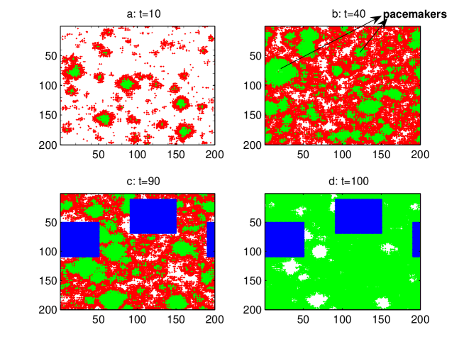
Figure 1: Spatial SIRS model simulation illustrating disease dynamics and aggregated vaccination. Parameters (as in [19]): $k=3,\tau_{I}=4,\tau_{R}=9,p=0.02,q=0.2$. (a) $t=10$. Circular waves of infected individuals (red) spread through a population of susceptible (white) and recovered/immune (green) individuals located in a $200\times 200$ lattice. (b) $t=40$. Data-analysis has identified two periodically reappearing pacemaker centers (red rings) of infected individuals. (c) $t=90$. Aggregated vaccination of all individuals (blue) located in proximity to the pacemaker centers - comprising only $18\%$ of the entire population. (d) $t=100$. Disease rapidly brought to extinction (all red infectives eliminated) in absence of other pacemaker centres.

When considering the population dynamics of STD’s it is important to take into account that some individuals spread the disease to a much greater extent than others. In this way, social behavior and sexual promiscuity governs the heterogeneity of the contact structure in the population. This contrasts with standard mean field differential equation models which are based on the assumption of a ”randomly mixing” population and lack a heterogeneous contact structure. However, there is no unanimous agreement on how the contact structure of the network should be fixed. Barabasi et al. [20, 21] have argued that ”scale free” networks, whose nodes have a power law connectivity distribution, are the most appropriate for STD’s. Lloyd and May [11], on the other hand, suggest that such a formulation is unnecessarily exaggerated. We follow Eames and Keeling [3, 4] who use a small world model as a first approximation for STD’s. Their model assumes that STD’s are generally transmitted locally but long-range infection pathways exist and are important in spreading the disease through the population network. Moreover, the small world approach creates heterogeneity in the connectivity distribution with most individuals having several connections, but some being more connected than others.

The small-world formulation is used here to study the spatio-temporal SIRS dynamics of recurrent diseases with temporal immunity. We first describe the network model and its spatio-temporal dynamics. For representative parameters the model exhibits expanding circular waves of infection, some of which are generated by unusual ”pacemaker centers”. These we study in detail; the important role of such ”pacemakers” suggests a practical disease control strategy based on targeted vaccination. We show that by vaccinating or quarantining the regions around pacemaker centers, the disease can be eradicated. The vaccination scheme is tested on various more realistic modifications of the basic model. We then formulate a very simple difference equation model that captures some of the main features of the heterogeneous network.

1 The network SIRS model

The network model is based on a $2-$dimensional lattice of individuals (/nodes) whose connectivity $p$ can be preassigned. Each node on the lattice is occupied and is connected to $k$ nearest neighbors oriented in each of four directions (North, South, East, West, with diagonal connections excluded). That is, each node is initially connected to $K=4k$ nearest neighbors, with $k=3$ unless otherwise specified. The horizontal and the vertical edges of the lattice are “glued” together creating a $2-$torus. Then, with a probability $p$, each of the $K$ nearest neighbors of each of the edges in the lattice is randomly rewired to an arbitrary node. These rewired connections, or “short-cuts” [18, 19], may extend to far regions of the network.

The parameter $p$ controls the population’s connectivity structure: $p=0$ corresponds to nearest neighbor contacts only, and where clustering is at its maximum; small $p$ in the range $0<p<0.1$ corresponds to a “small world” network (each individual has a certain amount of nearest neighbor contacts + a small proportion of distant contacts, “short-cuts”); large $p>0.4$ is qualitatively equivalent to a randomly mixing population with minimal clustering [19]. As $p$ is the probability of a short-cut, it may be viewed as an index of population mobility. Alternatively, it may be interpreted as an index of social behavior such as sexual promiscuity in the case of STD’s, given the manner in which it controls overall network connectivity and clustering [18].

Disease dynamics follow the classical Susceptible-Infectious-Recovered-Susceptible (SIRS) formulation [1, 22, 19, 3, 14] with Susceptible individuals ($S$) having a probability $q$ of becoming infected when linked to an Infected individual ($I$). Infected individuals eventually recover from the disease after a fixed time period, $\tau_{I}$, and are conferred temporary immunity. After a time period of $\tau_{R}$ time units, immunity wears off and Recovered individuals ($R$) return once again to the Susceptible pool ($S$) closing the SIRS loop.

This is implemented on the network using a $2-$dimensional cellular automata (CA), SIRS spatial model. At time $t$, an individual at the $(i,j)$’th location of the lattice has the state $x_{i,j}(t)$ which is either $S,I$ or $R$. The model is based on the following transition rules:

$$x_{i,j}(t)\in S\rightarrow\left\{\begin{array}[]{cc}x_{i,j}(t+1)\in I&with\quad prob.\quad 1-(1-q)^{k_{\inf}}\\ x_{i,j}(t+1)\in S&otherwise\end{array}\right.$$ (3)

$$x_{i,j}(t)\in I\longrightarrow x_{i,j}(t+1)\in I\rightarrow\cdot\cdot\cdot\longrightarrow x_{i,j}(t+\tau_{I})\in R$$

$$x_{i,j}(t)\in R\rightarrow x_{i,j}(t+1)\in R\rightarrow\cdot\cdot\cdot\longrightarrow x_{i,j}(t+\tau_{R})\in S.$$

Infections are transmitted to susceptible individuals with a probability $q$, if they are connected to an infective via a nearest neighbor or a short-cut. Thus the probability that a susceptible becomes infected is $1-(1-q)^{k_{\inf}}$, where $k_{\inf}$ is the total number of infected neighbors of the individual, be they connected via nearest neighbors or via short-cuts. The proportion of $S(t),I(t)$ and $R(t)$ individuals are calculated over the lattice and their dynamics are followed as a function of time.

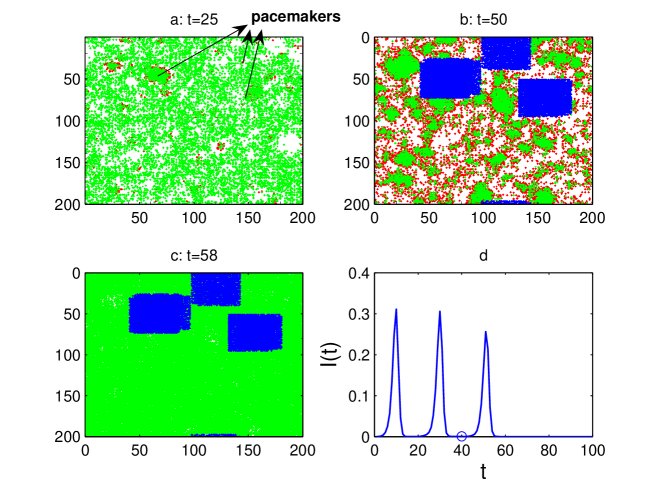
Figure 2: Model simulation of syphilis dynamics (3); white - susceptibles, red - infected, green - recovered, $k=3$, $\tau_{I}=6$ months, $\tau_{R}=4-8$ years, $p=0.065$, $q=0.36$, $\varphi=0.2$ p.y., $\mu=0.02$ p.y. (a) Three pacemakers are seen at time $t=12.5$ years. (b) Pacemaker areas are vaccinated with random spread of $86\%$ of each pacemaker area on average, at $t=41$ ($20.5$ years), resulting in vaccinating $14.5\%$ of the population. (c) Disease eradication at $t=58$ ($28$y.). (d) Time series of the proportion of infectives per $0.5$y. The period of oscillation is $T\thickapprox 10y$. The vaccination time is indicated by ’o’, after which the disease undergoes another smaller peak, and reaches complete extinction within less than one period of the disease ($8.5$ years).

To help fix ideas, we focus on two representative parameter settings: (a) parameters used in a general theoretical model taken from [19]. The infectious period is fixed at $\tau_{I}=4$ time units and a recovery period of $\tau_{R}=9$ time units (see simulations in Fig. 1); (b) parameters associated with syphilis epidemics as based closely on the study of Grassly et al. [14] (see simulations in Fig. 2). In the latter case $\tau_{I}=1$ time unit, which is taken to correspond to half a year; the recovery time varies randomly and uniformly in the range $\tau_{R}\in\{8,9,10,...,16\}$ time units corresponding to a period of $4-8$ years of immunity. To add realism, several other features are also incorporated. A birth-death process is introduced at rate $\mu$, indicating the proportion of births/death per time step with appropriate network rewiring. In Fig. 2, $\mu=0.01$ per half-year time step, which is equivalent to a rate of $\mu=0.02$ per year. Provision is made for the possibility that a proportion $\varphi$ of individuals fail to gain immunity after infection (similar to [14]). Thus $\varphi=0$ corresponds to all nodes passing through an SIRS loop while $\varphi=1$ corresponds to all nodes exhibiting SIS dynamics (no individual can acquire immunity). In Fig. 2 a proportion of $\varphi=0.2$ of the population ($20\%$) gaining no immunity per year.

1.1 Recurrent circular waves and pacemaker centers

We have found that in the small world regime, models of type (3) exhibit concentric waves which give rise to unusual “pacemaker centers.” Indeed, for $0.001<p<0.15$, the model (3) exhibits spatial oscillations with expanding circular waves of infection traveling through the lattice (see Fig. 1a). Some of these waves are recurrent, both spatially and temporally. The latter are generated by pacemakers (Figs. 1b and 2a) that form at connectivity centers - localized areas denser in short-cuts. The waves grow in size about the pacemakers as the infection spreads radially. When infected individuals recover, the interior of the growing wave boundary becomes a fresh pool of susceptible individuals. At the end of the cycle, a distant infectee “short-cuts” through the network to reinfect the wave’s focal pacemaker, enabling it to perpetuate. The cycle allows recurrent spatial waves to propagate with a fixed period, $T$. For the syphilis parameters (see Fig. 2 legend), $T\thickapprox 10$ years, as observed in US syphilis datasets [14, 23]. Similar spatial wave patterns had been observed in a number of biological contexts including epidemiology [24], ecology [25], neural networks [26] and theoretical studies of excitable systems [27].

These pacemakers follow a pattern formation mechanism. We observe that there is a minimal necessary amount of short-cuts needed for the creation of a pacemaker center. In addition, within the small-world range, a pacemaker wave region has more short-cuts than a non-pacemaker wave region.

The initiation of a pacemaker also requires that the infection is able to spread both in the horizontal and in the vertical directions. That is, the development of the infection from an initial state should progress in the two directions spanning a plane (i.e., in an X or an L shape). This condition follows the rule that heterogeneities are needed for creation of spirals in excitable media (see [27]). For these reasons, having an aggregation of short-cuts in a small region enhances the likelihood of creating a pacemaker. On the other hand, having too large an aggregation of short-cuts in a localized area of the lattice results in the opposite effect - disease extinction will occur in this localized area due to a synchronization effect (see [28] and below).

1.2 A Targeted Vaccination Scheme

The important role of “pacemaker centers” suggests a practical control strategy. We have found that by vaccinating or quarantining the regions surrounding pacemakers, the disease can be usually brought to a complete extinction within one period of the disease (in some cases, depending on the refinement of the vaccination algorithm and specific parameter values, two vaccination pulses are required). Thus, rather than the conventional scheme of immunizing some $85\%$ of the population to achieve herd immunity [1], it is only necessary to vaccinate groups enclosing the pacemakers. This requires vaccination of some $10\%-30\%$ of the population (depending on the specific application and algorithm refinement; $~{}\thicksim 20\%$ in most cases). Fig. 1 and Fig. 2 show spatial snapshots of an infected population upon application of the vaccination scheme. In the first frames (subfigs. 1a,b and 2a) the characteristic circular waves of infection (red) are seen. Vaccination around the pacemakers leads to complete eradication of the disease. Pacemakers have such large impact on the spatial dynamics that they are relatively easy to detect using a simple threshold algorithm that identifies recurring aggregations of infected individuals. Once a pacemaker is identified, a small region enclosing the pacemaker is marked out and vaccinated by effectively removing these nodes from the simulation (the blue rectangles in figures 1c,d and 2b,c).

For the theoretical values of [19] used in the simulations of Fig. 1, the ratio $\tau_{I}/\tau_{R}=4/9$ is relatively large, hence the pacemakers are large in size and few in number (usually $1-3$). In some cases, the scheme is able to remove all pacemakers after one application with vaccinating less than $10\%$ of the population. However, as the “pacemakers” compete with one another, there are cases where only the main pacemaker(s) is removed and secondary pacemaker(s) may appear in the next period. Eradication then requires a second application of the vaccination in the area of the remaining pacemaker(s). As shown in figure 1c,d, in such cases it typically requires vaccinating a total of some $18\%$ of all individuals over both applications to bring the disease to total extinction.

For the same model with syphilis parameters, the ratio $\tau_{I}/\tau_{R}$ varies in a simulation within the range $\{1/8,...,1/16\}$. As this ratio is small and variable, the pacemakers generated are more numerous (usually $2-5$) and smaller in size. The additional model realism ($20\%$ of the population not gaining any immunity, birth/death process) makes the pacemakers “less circular” in shape (see Fig. 2a). As a consequence, it is necessary to vaccinate more areas, although each area is smaller in size. Nevertheless, the vaccination scheme generally eradicates the disease in a single application, requiring vaccination of $14\%-22\%$ of individuals (see Fig. 2). As in practice it is difficult to obtain full coverage when vaccinating an entire population, or even a specific targeted group, to add realism (and lower vaccination rates) we vaccinated in Fig. 2 only an average of $86\%$ of each of the identified areas, enclosing pacemakers. In more detail, the algorithm vaccinates up to $98\%$ in the core of the pacemaker, where the high clustering of repeatedly infected individuals reside and as low as $60\%$ (randomly chosen) in the outskirts of the pacemaker.

It is of interest to examine the effects of simple random vaccination of the population. For the theoretical parameter values (a) based on [19] and used in Fig. 1, the random scheme is only successful in eradicating the disease after vaccinating at least $80\%$ of the population. For the syphilis parameter values, however, the random vaccination threshold is $43\%$ of the population (this is somewhat similar to the results presented in [29] for an SIR model). Hence, a further gain can be achieved by combining random vaccination with the targeted scheme above. This advantageously reduces the vaccination threshold to some $10\%-15\%$ of the population for the syphilis parameters. Instead of vaccinating the entire area surrounding the pacemaker it suffices to randomly vaccinate only $60\%$ of the area normally targeted.

In reality, this control scheme may be implemented by vaccination, quarantine or a targeted education plan, depending on the disease and on the means available for it’s control (for information on efforts to eliminate syphilis in the US see [15] and CDC reports [23]). The main advantage of the vaccination methods proposed here is that they avoid the usual practice of vaccinating a large proportion of the population. In addition vaccination is confined solely to relatively small and specified areas (see figures 1c,d and 2b,c). In practice, it is always preferable to vaccinate as small a group as possible, as vaccination always carries a risk. Hence, it is advantageous to target only the relevant groups, already at risk. In the case of syphilis, a vaccine [30] is still under development, but it is feared to be of relatively high risk - so if at all, vaccinating only carefully targeted population already at risk (e.g., in proximity to core groups of highly active individuals [31, 3]) will be desirable if and when such a vaccine is available. Note, however, that while other works refer to tracing infected individuals or the most connected individuals for applying a targeted vaccination scheme (e.g., [29, 32, 3]), in the scheme proposed here no contact tracing is required - the pacemaker waves stem from the SIRS dynamics and the small world structure in a natural and intrinsic way. Hence, these areas are easily identified as small areas where the infection appears repeatedly (see Figs. 1 and 2).

1.3 Synchronization and disease extinction

Worthy of comment is the model’s behavior for larger values of $p$, typically $p>0.1$, outside the “small world” regime, and corresponding to high levels of sexual promiscuity in the case of STD’s. Counterintuitively, the epidemic consistently dies out abruptly due to the appearance of large-scale synchronized epidemics [19, 28, 25] – a well known cause of disease extinction. The synchronization manifests with the formation of large spatial aggregations of infected individuals. Upon recovery, these infectives gain temporary immunity for a lengthy time period. Thus the areas that once contained aggregations of infectives, become exhausted of susceptibles and there is no possibility for an epidemic to sustain – it soon dies out.

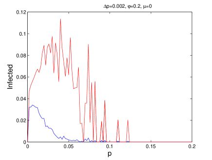
Figure 3: A bifurcation diagram of the proportion of infectives $I$ for typical syphilis parameter values (as in Fig.2) as a function of shortcuts $p$. For small $p$ there is an endemic equilibrium. After a bifurcation point the dynamics exhibit a limit cycle with radius varying with $p$. The diagram plots the maximum and minimum values of $I$ on the cycle. After a second bifurcation value of $p$ the disease goes to extinction (due to synchronization).

Although it might at first seem unusual, the model implies that for society at large, grand sexual promiscuity has the potential to eliminate STD’s such as syphilis altogether after about two decades of consistent behavior (see Fig. 3 and Fig. 4(c)). The same would be true for populations in which individuals consistently have few proximate sexual partners. The most conducive conditions for the persistence of such STD’s, appears to be the small world structure similar to the varying manifestation of sexual promiscuity seen in western society over the last centuries.

1.4 The impact of short-cuts

The effect of the parameter $p$ – the proportion of short-cuts, on the disease dynamics, may be assessed from the bifurcation diagram in Fig. 3. The figure plots the range in the number of infectives (maximum and minimum values) for any given $p$, when the model is run using the standard syphilis parameters. The following bifurcation scenario takes place: for $p=0$ the disease goes to extinction; for small $p<0.001$ an endemic equilibrium is reached in which there is a relatively small proportion of infectives $0<I^{*}\ll 1$; for $0.001<p<0.13$ (approximately) there is a limit cycle of radius depending on $p$ and hence noticeable oscillations in the number of infectives; for $p\gtrsim 0.13$ the disease goes to extinction due to a synchronization effect. The “limit cycle region” is the region where pacemaker centers develop and within it lies the region where the targeted vaccination scheme works very effectively. This region is an open strip of $p$ values in the “small world” regime. Note that both for $p=0$ and for large $p$ the disease rapidly goes to extinction. Thus, despite the period of temporary immunity built into this model, oscillations in $I$ vanish for either very small or relatively large values of $p$ (i.e., outside the small world regime).

2 Difference equation model

We formulate the following difference equation model to help gain insights into the network model’s dynamics. Let $S_{t}$, $I_{t}$ and $R_{t}$ be the proportion of susceptible, infective and recovered individuals in a large population at time $t$. Again, let $\tau_{I}$ be the time period an individual remains infectious and $\tau_{R}$ the period an individual remains immune. If we assume that $\tau_{I}=1$, as the case for syphilis, the proportion of recovered individuals can be described by the sum: $\Sigma_{i=1}^{\tau_{0}-1}I_{t-i}$, and thus:

$$S_{t}=1-I_{t}-\Sigma_{i=1}^{\tau_{0}-1}I_{t-i},$$ (4)

where $\tau_{0}=\tau_{I}+\tau_{R}$. The above model formulation is well known (see e.g., [33]), but is extended as follows. We suppose each individual has on average $K$ connections including those to nearest neighbors and short-cuts. For the typical individual, denote by $K_{t}^{\inf K}$ the number of nearest neighbors that are infected at time $t$ and denote by $K_{t}^{\inf p}$ the number of short-cut links that point to infected individuals. Then:

$$K_{t}^{\inf K} = I_{t}(1-p)K,$$ (5)

$$K_{t}^{\inf p} = I_{t}pK.$$ (6)

Set $q_{p}$ as the probability of being infected by a short-cut link and set $q_{K}$ as the probability of being infected by a nearest neighbor. In practice $q_{p}>q_{K}$, because of the important role short-cuts play in spreading the epidemic through the network. For example, simulations of the lattice model (Eqn. 3) under syphilis parameters show that $q_{p}\thicksim 4q_{K}$. For the model parameterized with the theoretical values taken from [19], $q_{p}\thicksim 10q_{K}$. Incorporating this important observation in the difference equation leads to the following model of the $SIRS$ dynamics on a complex contact network:

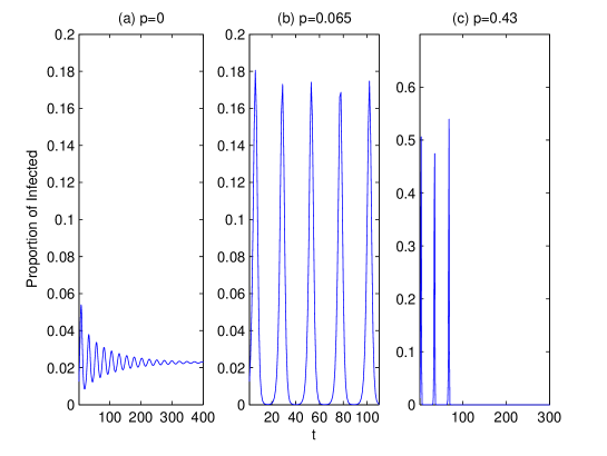
Figure 4: Time series of the difference equation model (7) for different $p$ values close to bifurcation points; $qK=0.11$, $qp=0.65$, $K=12$.

$$I_{t+1}=(1-(1-q_{K})^{K_{t}^{\inf K}}(1-q_{p})^{K_{t}^{\inf p}})S_{t},$$ (7)

where $q_{K}<q_{p}\leq 1$. Note that equation (7) captures both the time delay dynamics resulting from the temporary immunity of the disease and the social effects of the short-cuts.

The dynamics of the model (7) depend on $p$ in a manner that is very similar to the more complex contact network model (3). Fig. 4 shows results based on setting $q_{K}=0.11$ and $q_{p}=0.65$. For $p=0$, a small endemic equilibrium is reached (see Fig. 4(a)), for $p$ in the small world range sustained oscillations arise (see Fig.4(b)) 4(b)), and for large $p$ the disease is eradicated (see Fig. 4(c)) due to a synchronization effect. Comparing figures 2d and 4(b) 4(b) – one can see exactly the same type of dynamics with similar period of about $10$ years, as observed in syphilis datasets [23, 14].

2.1 Stability analysis

The equilibrium solutions of model (7) are found by solving the following equation for $I^{\ast}$:

$$I^{\ast}=(1-(1-q_{K})^{I^{\ast}(1-p)K}(1-q_{p})^{I^{\ast}pK})(1-\tau_{0}I^{\ast}).$$ (8)

It is easily seen that the infection-free equilibrium $I^{\ast}=0$ is always a solution. A stability analysis (based on linearizion of Eqn. 7) reveals that the infection-free equilibrium is stable when the following inequality holds:

$$R_{0}=-K[{(1-p)\ln(1-q_{K})+p\ln(1-q_{p})}]\leq 1.$$ (9)

Hence, for the given model parameters and relevant $K$ values ($K=8$ or $12$), the infection free equilibrium is stable either only for extremely small $p$ values ($K=8$), or never ($K=12$). This is visualized in Fig. 5(a) which plots the bifurcation curve of the infection free equilibrium as a function of the parameters $K$ and $p$. The infection free equilibrium is stable for all values of parameters below the (lower solid) curve where $R_{0}<1$ and unstable otherwise since $R_{0}>1$. For $K\leq 4$, the infection free equilibrium is stable in a wide strip of the parameter plane, containing the small world regime (as visible in Fig.5a).

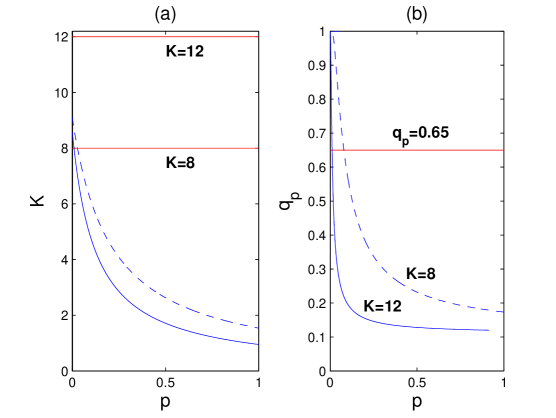
Figure 5: Bifurcation diagrams of the difference equation [7]; $\tau_{0}=11$, $q_{K}=0.11$. (a) $q_{p}=0.65$. Infection free equilibrium $(I^{*}=0)$ is stable for parameters below solid curve along which $R_{0}=1$. Dashed curve is the approximation based on estimating $R_{0}$ (see text). (b) Hopf bifurcation curves. Endemic equilibrium is stable for parameters below indicated curves and a stable limit cycle is born when these curves are crossed (solid curve: $K=12$, dashed curve: $K=8$).

A similar result is obtained by estimating the reproductive number $R_{0}$, approximating it as the average number of secondary infectives produced by a typical infective individual in a sea of susceptibles. In the case here, where a single node may infect only those nodes it is linked to, the number of secondary infections may be approximated as:

$$R_{0}\approx K(q_{K}(1-p)+q_{p}p).$$ (10)

The above estimate gives a good approximation of the exact condition (9) as seen in in Fig. 5(a) (dashed curve).

For most parameter values, the difference equation (7) has a second endemic equilibrium in which $I^{\ast}>0$. The bifurcation curves describing it’s stability in the $(p,q_{p})$ parameter plane are shown in Fig. 5(b), for $K=8$ (upper curve) and $K=12$ (lower curve). This curve indicates a Hopf bifurcation in the $(p,q_{p})$ plane, where all other parameters are kept fixed. See Appendix1 for technical details on its calculation. The endemic equilibrium exists for all parameter values for which the Hopf bifurcation curve exists. Below the bifurcation curve the endemic equilibrium is stable and is unstable above it, where a stable limit cycle exists. The stable limit cycle thus coexists with the two unstable equilibria – infection free and endemic.

Hence, the bifurcation scenario, for syphilis parameter values, for $K=8$, is as follows. For $0\leq p\leq 0.0091$, the infection free equilibrium is stable and the disease goes extinct; for $0.0091<p\lesssim 0.079$ the infection free equilibrium loses it’s stability and an endemic equilibrium is born; for $p\gtrsim 0.079$ the endemic equilibrium loses it’s stability through a Hopf bifurcation and a stable limit cycle is born. See the upper dashed Hopf bifurcation curve in Fig. 5(b). In the case of $K=12$, the infection free equilibrium is unstable for all values of $p$. However, the endemic equilibrium is stable for $0\leq p\lesssim 0.011$. When $p\gtrsim 0.011$, both equilibria are unstable and instead a stable limit cycle is observed. See the lower solid Hopf bifurcation curve in Fig. 5(b).

As in the network model, the disease goes completely extinct for relatively large $p$ values (for $K=12$, $p_{c}=0.43$ and for $K=8$, $p_{c}=0.87$), despite the fact that the infection free equilibrium is unstable (see Fig. 4(c)). The extinction should be attributed to the synchronization effect that takes place for these high $p$ values. That is, the dynamics are such that a large proportion of the population become infected together and proceed on to move to the recovered class together. The synchronization requires the initiation of a strong epidemic, implying that $R_{0}$ must be greater than unity, which explains why the infection free equilibrium is unstable in this regime. Nevertheless the disease becomes extinct due to the synchronization effect.

2.2 Vaccination

A random vaccination scheme may be incorporated into the difference equation model by replacing $S_{t}$ in Eqn. (7) with $(1-v)S_{t}$. The parameter $v$ is the proportion of susceptibles vaccinated per time unit. Denote by $v_{e}$ the threshold proportion of vaccinated needed for disease extinction. A simple algebraic expression can be obtained for the extinction threshold by linearizing Eqn. (7) about the infection free equilibrium. Then, by using equation (9), disease extinction is reached if:

$$v\geq v_{e}=1-\frac{1}{R_{0}}.$$ (11)

For the parameter values of Figs. 4 and 5, the vaccination threshold is $v_{e}=0.5297$. Numerical simulations corroborate the existence of this threshold.

As the difference equation does not give any information regarding spatial patterns, it is impossible to apply the spatially oriented targeted vaccination scheme described above. However, targeted vaccination schemes may nevertheless be explored by differentiating between vaccinating nearest neighbors and short-cuts. This can be achieved by replacing the term $I_{t}$ in equations (4) and (7) with the term $(1-v_{K})I_{t}$ for nearest neighbors and $(1-v_{p})I_{t}$ for short-cuts. The results reveal that the extinction threshold is very sensitive to and lowered dramatically by the term $v_{p}$ for vaccinating short-cuts, while the term for vaccinating nearest neighbors, $v_{K}$, has little influence. Although according to the model the infection free equilibrium is never stable for the syphilis disease in a small world type society, it appears that targeted vaccination effectively reduces the number of the actual contacts of the key individuals, thereby reducing $R_{0}<1$ in the vaccinated population. A detailed study of the targeted vaccination is left for future work.

3 Conclusion and discussion

Two models for studying the dynamics of diseases with temporary immunity in complex population networks have been proposed – a lattice model, which incorporates spatial information, and a difference equation model, which allows an analytic approach. The study focuses on the example of syphilis epidemics, which is a representative STD targeted to be eliminated in the US with little success so far. The network model reveals that diseases with temporary immunity on a small world contact network exhibit periodicity and waves of epidemics, some of which become pacemaker centers. It is shown that by eliminating pacemakers through vaccination, the disease goes to extinction within $1-2$ periods, where only about $20\%$ of the population requires vaccination. This is in contrast to standard vaccination programs that set out to achieve herd immunity by vaccinating over $80\%$ of the population. Moreover, by treating only those individuals in high risk pacemaker areas, it minimizes the application of the vaccination with its possible risks to the larger population. The difference equation model allows further investigation of the Hopf bifurcation lying at the heart of the pacemaker phenomena. The models presented here were constructed in accordance to the US syphilis datasets (see [23, 16] and [14]). The two models complement each other, allowing a more profound view of the dynamics.

This work addresses the controversy as to whether syphilis epidemics recur approximately every ten years due to the temporary immunity it endows to infected individuals ([14]) or due to changing patterns in social behavior ([23, 16]). As shown here, both factors are crucial for recurrent syphilis epidemics. Thus, for example, oscillations cannot occur outside the small world regime even in the presence of strong temporary immunity. For zero or very small $p$ values (corresponding to none, or a very few, short-cut links), an epidemics cannot develop. Moreover, the analysis performed on the difference equation model reveals that if all individuals in a small world type population network have only a small number of contacts, the infection free equilibrium is stable. In addition, on the other side of the scale, it is pointed out that for large enough $p$ outside the small world region (corresponding to many short-cut links) a synchronization effect takes place, eradicating the epidemics due to exhaustion of susceptibles. In contrast, a society whose social behavior approximates a small world network with moderate heterogeneous levels of promiscuity would sustain the periodic recurrences of the syphilis epidemics approximately every ten years.

Finally, we conjecture that complete disease extinction is nevertheless achievable by a targeted vaccination scheme similar to that presented here. The targeting and vaccination of key individuals, effectively reduces $R_{0}$ to less than unity in the vaccinated population, thereby leading to disease extinction.

Appendix A Appendix1: Technical details for the difference equation model

Here we present the technical details of the stability analysis performed for the difference equation model (7). Consider the Susceptible - Infectious - Recovered - Susceptible (SIRS) dynamics. Assume $\tau_{I}$ is the amount of time units an individual spends in the Infectious class and that $\tau_{R}$ represents the time units an individual later spends in the Recovered class. As for syphilis $\tau_{I}=1$ (where a time unit represents $6$ months), the proportion of recovered individuals can be described by the sum: $\Sigma_{i=1}^{\tau_{0}-1}I_{t-i}$. Thus, denoting by $S_{t}$ the proportion of susceptibles in the population at time $t$, we obtain:

$$S_{t}=1-I_{t}-\Sigma_{i=1}^{\tau_{0}-1}I_{t-i},$$ (12)

where $\tau_{0}=\tau_{I}+\tau_{R}$. Set $I_{t}$ to be the proportion of infectives at time $t$, denote by $K$ the number of connections an individual has on average and let $p$ be the proportion of short-cut links an individual has among it’s $K$ connections. Then, denote by $K_{t}^{\inf K}$ the number of infectious nearest neighbors an individual node has at time $t$ and by $K_{t}^{\inf p}$ the number of infectious contacts via short-cut links an individual node has among its $K$ connections at time $t$. Then:

$$K_{t}^{\inf K} = I_{t}(1-p)K,$$ (13)

$$K_{t}^{\inf p} = I_{t}pK.$$ (14)

Set $q_{p}$ as the probability of being infected via a short-cut link and set $q_{K}$ as the probability of being infected by a nearest neighbor, where $q_{K}<q_{p}<1$. Hence, the $SIRS$ dynamics on a network with nearest neighbors and short-cut connections can be described by:

$$I_{t+1}=(1-(1-q_{K})^{K_{t}^{\inf K}}(1-q_{p})^{K_{t}^{\inf p}})S_{t},$$ (15)

The dynamics of (15) are at equilibrium for the solutions, $I^{\ast}$, of the equation (16):

$$I^{\ast}=(1-(1-q_{K})^{I^{\ast}(1-p)K}(1-q_{p})^{I^{\ast}pK})(1-\tau_{0}I^{\ast}).$$ (16)

It is easily seen that the infection free equilibrium $I^{\ast}=0$ is always a solution and that an endemic equilibrium $I^{\ast}>0$ is a solution for most parameters relevant for syphilis.

Substituting $J_{t}=I_{t}-I^{\ast}$ and linearizing Eqn.(15) about $I^{\ast}$, we obtain:

$$J_{t+1}=(1-q_{K})^{(1-p)KI^{\ast}}(1-q_{p})^{pKI^{\ast}}\left(R_{0}(1-\tau_{0})J_{t}+\Sigma_{i=0}^{\tau_{0}-1}I_{t-i}\right)-\Sigma_{i=0}^{\tau_{0}-1}I_{t-i}+h.o.t.,$$

where,

$$R_{0}=-K((1-p)\ln(1-q_{K})+p\ln(1-q_{p})).$$

Now substitute $J_{t}=J_{0}\lambda^{t}$ to obtain the characteristic polynomial,

$$\lambda^{\tau_{0}}+\alpha\lambda^{\tau_{0}-1}+\beta\lambda^{\tau_{0}-2}+\cdot\cdot\cdot+\beta\lambda+\beta=0,$$ (17)

where:

$$\alpha = (1-q_{K})^{(1-p)KI^{\ast}}(1-q_{p})^{pKI^{\ast}}\left(R_{0}(\tau_{0}I^{\ast}-1)-1\right)+1,$$ (18)

$$\beta = 1-(1-q_{K})^{(1-p)KI^{\ast}}(1-q_{p})^{pKI^{\ast}}.$$

The stability of the infection free equilibrium is derived from substituting $I^{\ast}=0$ and requiring that $\left|\lambda\right|=R_{0}<1$. The stability analysis of the infection free equilibrium is presented in the main text (and Fig. 5(a)). Here we provide details regarding the endemic equilibrium stability and the calculation of the Hopf bifurcation curve(s), presented in Fig. 5 in the main text. This calculation is inspired by a calculation of the Hopf bifurcation of a mean field difference equation model in [33].

Assume such a bifurcation exists and substitute $\lambda=e^{i\phi}$ (as stability changes at $\left|\lambda\right|=1$) into Eqn.(17). Separating real and imaginary parts we obtain two equations:

$$\alpha = -\cos(\phi)-\cot\left(\frac{\phi\tau_{0}}{2}\right)\sin(\phi),$$ (19)

$$\beta = \frac{2\csc\left(\frac{\phi\tau_{0}}{2}\right)\sin\left(\frac{\phi}{2}\right)\sin(\phi)}{\cos\left(\frac{\phi(\tau_{0}-2)}{2}\right)-\cos\left(\frac{\phi\tau_{0}}{2}\right)}.$$

Substituting Eqns.(18) into Eqns.(19) and adding Eqn.(16) results in a system of three equations in the seven variables: $q_{K},q_{p},p,K,I^{\ast},\tau_{0},\phi$. Some of these parameters can be fixed to values relevant for syphilis: $\tau_{0}=11$, $K=8$ or $12$ and $q_{K}=0.11$. $\phi$ can be viewed as the frequency of the periodic solution emerging at the bifurcation, where the period of the limit cycle (when exists) is $T\thickapprox\frac{2\pi}{\phi}$. As for the syphilis parameter values the period of oscillation is $T\thickapprox 20$ time units, where $1$ time unit $=0.5y=6$ months, we fix $\phi=0.3$. Now, with these fixed parameter values, we use the Newton method to solve Eqns.(19) and (16), using the syphilis parameter values as the initial guess, once for $K=8$ (dashed curve in Fig. 5(b)) and once for $K=12$ (solid curve in Fig. 5(b)). The results are plotted in the $(p,q_{p})$ plane (see Fig. 5(b)  in the main text). In Fig. 5(b), the two bifurcation curves (one for $K=8$  - dashed and one for $K=12$ - solid) are presented, where below each curve an endemic equilibrium $I^{\ast}>0$ is stable. At the bifurcation curve the equilibrium loses its stability and a stable limit cycle is born so that above the curve a stable limit cycle coexists with two repelling (unstable) equilibria - the infection free and an endemic.

References

- [1] R.M. Anderson and R.M. May. Infectious Diseases of Humans: Dynamics and Control. Oxford University Press, New York, 1991.
- [2] S. Riley. Large-scale spatial-transmission models of infectious diseases. Science, 316:1298–1301, 2007.
- [3] K.T. Eames and M.J. Keeling. Modeling dynamic and network heterogeneities in the spread of sexually transmitted diseases. PNAS, 99(20):13330–13335, 2002.
- [4] M.J. Keeling and K.T.D. Eames. Networks and epidemic models. Interface, J. Roy. Soc., 2:295–307, 2005.
- [5] B.T. Grenfell, O.N. Bjornstad, and B.F. Finkenstadt. Dynamics of measles epidemics: scaling noise, determinism, and predictability with the tsir model. Ecol. Mon., 72:185–202, 2002.
- [6] D.J.D. Earn, P. Rohani, B.M. Bolker, and B.T. Grenfell. A simple model for complex dynamical transitions in epidemics. Science, 287:667–670, 2000.
- [7] P. Rohani, D. J. D. Earn, and B. T. Grenfell. Opposite patterns of synchrony in sympatric disease metapopulations. Science, 286:968–971, 1999.
- [8] S. Eubank, H. Guclu, V. S. A. Kumar, M. V. Marathe, A. Srinivasan, Z. Toroczkai, and N. Wang. Modelling disease outbreaks in realistic urban social networks. Nature, 429:180–184, 2004.
- [9] H.W. Hethcote and J.A. Yorke. Gonorrhea: transmission dynamics and control. Lect. Notes Biomath., 56:1–105, 1984.
- [10] J.N. Wasserheit and S.O. Aral. The dynamic topology of sexually transmitted disease epidemics: implications for prevention strategies. J. Infect. Dis.1996;, 174(2):S201–S213, 1996.
- [11] A. L. Lloyd and R. M. May. How viruses spread among computers and people. Science, 292:1316–1317, 2001.
- [12] S. A. Levin, T. G. Hallam, and L. J. (Eds.) Gross, editors. Applied Mathematical Ecology. Springer Verlag, 1989.
- [13] N. M. Ferguson, A. P. Galvani, and R. M. Bush. Ecological and immunological determinants of influenza evolution. Nature, 422:428–433, 2003.
- [14] N.C. Grassly, C. Fraser, and G.P. Garnett. Host immunity and synchronized epidemics of syphilis across the United States. Nature, 433:417–421, 2005.
- [15] M.E. St. Louis and J.N. Wasserheit. Elimination of syphilis in the United States. Science, 281:353–354, 1998.
- [16] J.M. Douglas. Jr. MD, Director, Division of STD Prevention, Letter to CDC and Cyclical Syphilis Letter to the Editor. http://www.cdc.gov, Feb 2005.
- [17] M. E. J. Newman. The structure and function of complex networks. SIAM Review, 45:167–256, 2003.
- [18] D.J. Watts and S.H. Strogatz. Collective dynamics of ’small-world’ networks. Nature, 393:440–442, 1998.
- [19] M. Kuperman and G. Abramson. Small world effect in an epidemiological model. Phys. Rev. Lett., 86(13):2909–2912, 2001.
- [20] A.-L Barab si and R. Albert. Emergence of scaling in random networks. Science, 286:509–512, 1999.
- [21] F. Liljeros, C. R. Edling, L. A. N. Amaral, H. E. Stanley, and Y. berg1. The web of human sexual contacts. Nature, 411:907–908, 2001.
- [22] J.D. Murray. Mathematical Biology, volume 17 of Interdisciplinary Applied Mathematics. Springer,, 2002, third edition.
- [23] CDC. Reports: Primary and Secondary Syphilis – US, 1997, in MMWR Weekly 47(24) (1998). Syphilis Elimination Effort report and updates (2005). http://www.cdc.gov, 1997-todate.
- [24] B.T. Grenfell, O.N. Bjornstad, and J. Kappey. Travelling waves and spatial hierarchies in measles epidemics. Nature, 72:716–723, 2001.
- [25] B. Blasius, A. Huppert, and Stone L. Complex dynamics and phase synchronization in spatially extended ecological systems. Nature, 399:354–359, 1999.
- [26] T.J. Lewis and J. Rinzel. Self-organized synchronous oscillations in a network of excitable cells coupled by gap junctions. Network: Comput. Neural Syst., 11:299–320, 2000.
- [27] J.M. Greenberg and S.P. Hastings. Spatial patterns for discrete models of diffusion in excitable media. SIAM Journal on Applied Mathematics, 34(3):515–523, 1978.
- [28] D. J. D. Earn, P. Rohani, and B. T. Grenfell. Persistence, chaos and synchrony in ecology and epidemiology. Proc. R. Soc. B, 265:7–10, 1998.
- [29] D. H. Zanette and M. Kuperman. Effects of immunization in small-world epidemics. Physica A: Statistical Mechanics and its Applications, 309(3-4):445–452, 2002.
- [30] P. A Cullen and C. E. Cameron. Progress towards an effective syphilis vaccine: the past, present and future. Expert Review of Vaccines, 5(1):67–80(14), February 2006.
- [31] J.C. Thomas and M.J. Tucker. The development and use of the concept of a sexually transmitted disease core. J Infect Dis, 174(2):S134–S143, 1996.
- [32] R. Pastor-Satorras1 and A. Vespignani. Immunization of complex networks. Phys. Rev. E, 65:036104, 2002.
- [33] M. Girvan, D. S. Callaway, M. E. J. Newman, and S. H. Strogatz. A simple model of epidemics with pathogen mutation. Phys. Rev. E, 65(031915), 2002. nlin.CD/0105044.