From Protein Interactions to Functional Annotation: Graph Alignment in Herpes

Abstract

Sequence alignment forms the basis of many methods for functional annotation by phylogenetic comparison, but becomes unreliable in the “twilight” regions of high sequence divergence and short gene length. Here we perform a cross-species comparison of two herpesviruses, VZV and KSHV, with a hybrid method called graph alignment. The method is based jointly on the similarity of protein interaction networks and on sequence similarity. In our alignment, we find open reading frames for which interaction similarity concurs with a low level of sequence similarity, thus confirming the evolutionary relationship. In addition, we find high levels of interaction similarity between open reading frames without any detectable sequence similarity. The functional predictions derived from this alignment are consistent with genomic position and gene expression data.

Introduction

With the advent of genome-wide functional data, cross-species comparisons are no longer limited to sequence information. A classic extension of sequence alignment is structural alignment, which has been used to compare evolutionary distant RNAs  [1] and proteins conserved in structure rather than sequence [2, 3]. Here we use protein interactions as evolutionary information beyond sequence [4].

We perform a cross-species analysis of two herpes viruses, the varicella-zoster virus (VZV), causing chicken pox and shingles, and the Kaposi’s sarcoma-associated herpesvirus (KSHV), responsible for cancer of the connective tissue. The two viruses have diverged approximately $200$ million years ago. Their sequence dynamics is characterised by a high rate of point mutations (at least an order of magnitude faster than their host populations [5]) and a high rate of gain and loss of genes (an order of magnitude higher than the mutation rates of procaryotes [6]). As a result, the sequence similarity between the two species is in the “twilight” region of detection by alignment: homologous proteins have an amino acid sequence identity of about $20\%$. Moreover, many open reading frames are only about $60$ amino acids long.

The protein interactions in both species have recently been measured by a yeast two-hybrid screen [4]. Together with regulatory couplings, protein interactions are believed to be an important source of phenotypic change, possibly more so than the overall change of coding sequences [7, 8]. Protein interactions are encoded in mutually matching binding domains. The evolutionary dynamics of these domains is governed by different selection and hence, by different tempi than the overall coding sequence. Moreover, amino acids relevant for binding are difficult to localise from sequence data alone, and the sequence of a domain may evolve considerably while its interaction is conserved. Therefore, we treat the experimental interaction data as evolutionary information independent of sequence data. However, these data are noisy as well, not least due to the experimental difficulties of high-throughput measurements.

Our hybrid comparison method called graph alignment jointly uses the similarity of protein interactions and of coding sequences to establish a mapping between genes of two species [9]. The underlying evolution involves a number of distinct processes, including divergent sequence evolution, gain and loss of interactions, duplication of genes and the corresponding interactions, and gain and loss of genes. Functional relationships may stem from common ancestry and thus be detectable by sequence homology, but they may also arise by convergent evolution, this analogy displayed by similar interactions without sequence similarity. An example is given in Figure 1, where one gene has functionally replaced another gene by acquiring its interactions, a process called non-orthologous gene displacement [10]. Similarly, an orthologous gene pair may diverge in sequence beyond detectability, but conserved interaction patterns remain detectable due to functional constraints. Such functional relationships are deduced from the network of interactions between genes. Computationally, graph alignment rests on a probabilistic scoring system, which weighs the cross-species similarities of sequences and interaction networks based on their evolutionary rates. Our method simplifies in special cases: (i)  If gene sequences are well conserved and gene displacements are rare, one may restrict the map between genes or proteins to sequence homology (green lines in Figure 1) and, for example, identify network parts enriched in conserved links [11, 12]. (ii) Conversely, if sequence similarity has uniformly decayed below the significance threshold, one can construct a map between genes or proteins based solely on the interactions between them [13].

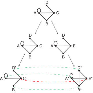
Figure 1: Detecting functional relationships by graph alignment. In this example, the gene labelled $C$ is replaced in one lineage with its functional equivalent $E$, which has the same interaction partners in the network. While some genes can still be correctly mapped across species using sequence information (green lines), the full evolutionary history and the mapping $C^{\prime}-E^{\star}$ are accessible from cross-species analysis only by taking into account the interaction networks.

For the graph alignment between the VZV and KSHV viruses studied in this paper, both the interaction networks and the gene sequences are crucial to determine functional relationships, while each part of the data by itself is often insufficient. In particular, we find protein pairs with low sequence similarity for which the interaction similarity strengthens the statistical inference of homology, as well as protein pairs without sequence similarity, which are aligned based on their interactions alone. We use this alignment to make functional predictions. These predictions turn out to be consistent with published experimental data where available.

Theory

Scoring graph alignments. We use a recently developed method for the alignment of graphs [9], adapted to the specific situation of sparse interaction networks with a low number of matching links. Open reading frames are represented by nodes, and pairwise protein interactions are represented by links between nodes. A graph alignment $\pi$ is a mapping of nodes of one network to nodes of the other network. The alignment is characterised by (i) interaction similarity of aligned nodes and (ii) sequence similarity of the aligned nodes.

Matching links in the two networks give a positive contribution to the score: aligned node pairs $i$ and $j=\pi(i)$, and $i^{\prime}$ and $j^{\prime}=\pi(i^{\prime})$ contribute a positive score if a link is present both between the pair $(i,i^{\prime})$ in one network and $(j,j^{\prime})$ in the other network. An example are the links between $D^{\prime}-C^{\prime}$ and $D^{\star}-E^{\star}$ in Figure 1. A negative contribution results if a link is present in one network, but not in the other (mismatched links, as $D^{\prime}-B^{\prime}$ and $D^{\star}-B^{\star}$ in Figure 1). The values of the link scores are encoded in the link scoring function $s_{l}(a,b)$ where $a\in{1,0}$ (link present or absent in one network), and likewise $b\in{1,0}$ (link present or absent in the other network). For binary links this scoring function is a $2\times 2$ matrix, conceptually related to the scoring matrices in sequence alignment. In addition to interaction similarity, the sequence similarities $\theta_{ij}$ between nodes contribute to the score, rewarding similarity between aligned pairs and penalising similarity between pairs not respected by the alignment.

The total graph alignment score is the sum of independent contributions from sequence similarity and from link similarity. As a result, a pair of nodes may be aligned because of high sequence similarity, or because of high node similarity, or both. Of course, the interplay between sequence similarity and link similarity depends crucially on the relative weight of node score and link score. These scoring functions are determined self-consistently from the data within a Bayesian framework, see supplementary text.

Graph alignment algorithm. We use an iterative algorithm described in [9] to find the graph alignment with maximal score, based on a mapping to the quadratic assignment problem. At each step the highest scoring alignment is identified individually for each node, while keeping the rest of the alignment fixed. A certain amount of noise is used to help the alignment to escape from local score maxima (as in simulated annealing [18]). This noise amplitude is gradually decreased to zero, starting from some initial value $T$ and an initial alignment of reciprocal best sequence matches.

Alignment regimes and method tests. We test our alignment procedure on correlated random graphs, comparable in size and average connectivity to the protein interaction networks of KSHV and VZV. Two such graphs are generated from a common ancestor graph by independently adding and deleting a certain fraction of links (see supplementary text for details). In addition, we specify the sequence similarities for a subset of the node pairs. The correct alignment maps all orthologous pairs, including those where no sequence information is specified.

For network pairs with high connectivity and high link similarity, the alignment is faithful and reproducible, independently of the noise level $T$. For example, given $80$ nodes with $60$ sequence orthologs specified, and $140$ links of which approx. $100$ match, the alignment reproduces all nodes with sequence orthologs and $70\%$ of those without. The finite recovery rate stems from node pairs lacking any matching links.

For network pairs with low link similarity, we find two different alignment regimes depending on the initial noise level $T$.

(i) In the high-fidelity regime for values of $T$ well below a threshold value $T_{D}$, the alignment consists mainly of the nodes with sequence similarity, but does not extend much beyond. For example, if only approx. 50 of 140 links match in the above network pair, the final alignment for $T=4$ contains all 32 node pairs with sequence similarity but only 4 node pairs without sequence similarity, all of which are correctly aligned.

(ii) In the low-fidelity regime for $T$ above $T_{D}$, high-scoring alignments contain many link matches (even more than in the correct alignment), but different runs have little overlap and most nodes (even with sequence similarity) are misaligned. Correspondingly, the alignment has a high link score and a low node score, see Figure 2(a). In the above example, only $29$ of $32$ nodes with sequence similarity are correctly aligned and as many as $14$ of $21$ nodes without sequence similarity are misaligned at $T=8$. This behaviour is generic to graph alignment, independent of score function and details of the algorithm. The high-scoring alignments in the low-fidelity regime are random islands of locally matching links. Their occurrence can be understood from the special case of two uncorrelated graphs with a narrow range of connectivities. Aligning a pair of randomly chosen nodes with each other, their neighbours, and their next neighbours, etc., will lead to a high link score (possibly offset to some extent by a low node score). There are many such alignments with a high score, yet low statistical significance. These spurious alignments occur for sparse networks at sufficiently low fractions of link matches and low numbers of nodes with sequence similarity. They are comparable to the score islands known in local sequence alignment [19], except that in graph alignment the number of such “islands” is much greater than in sequences.

(iii) Hence, optimal detection of similarity occurs in the high-fidelity regime for values of $T$ just below $T_{D}$; see Figure 2(b). In this region the alignment is still guided by sequence similarity, yet extends as much as possible into the set of nodes without sequence similarity. The corresponding ROC curve is shown in the supplementary text. In the above example, this conservative approach correctly aligns $5$ pairs of $48$ without sequence similarity for $T=5$, and there is no misalignment. The same way of choosing $T$ is applied to the real protein interaction network data.

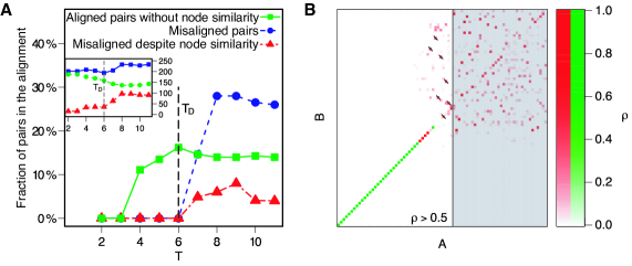
Figure 2: Testing the graph alignment: Artificial networks with low link similarity. a) Unlike in the case of high link similarity (see text), the alignment of networks with low link similarity depends on the noise parameter $T$ of the alignment algorithm. With increasing noise parameter $T$ a wider range of alignments is probed by the algorithm, leading to an increasing number of nodes correctly aligned from their link similarity alone (green $\square$-symbol). This heightened sensitivity is paid for with decreasing specificity: also the fraction of nodes aligned with a node different from their sequence homolog (red $\triangle$-symbols) and the ratio of misaligned nodes without sequence homolog (blue $\circ$-symbols) increase with $T$. Signature of the transition to the low-fidelity regime is the rapidly increasing link score (inset red $\triangle$-symbols) and the decreasing node score (inset green $\circ$-symbols) while the total score (inset blue $\square$-symbols) increases only slowly. However, just before the onset of the low-fidelity regime at $T=5$ correct alignments are obtained from network similarity alone with few incorrect alignments (in this case none).
b) The noise parameter of the algorithm is set just before the onset of the low-fidelity regime ($T=5$). The alignment is represented by the matrix $\rho$, with $\rho(i,j)$ indicating the relative frequency with which a node $i$ is aligned with $j$ over many alignment runs. The correct alignment $i=j$ lies along the diagonal. Entries of $\rho$ coloured green correspond to node pairs with mutual sequence similarity, those coloured red have no sequence similar partner and are aligned on the basis of link similarity alone. A cutoff of $\rho>0.5$ is used, and aligned node pairs with less than two matching links are discounted (crossed-out points). This leads to $5$ node pairs correctly aligned on the basis of their links only, and no misaligned node pairs. This is a conservative scheme, as can be seen by glancing along the diagonal for additional entries with lower values of $\rho$.

Results

Optimal graph alignment between VZV and KSHV. The protein interaction network of the herpes virus VZV consists of $76$ Orfs and $173$ protein-protein interactions (of these Orfs, $19$ have no detected interactions and are disregarded from the subsequent analysis). The protein interaction network of KSHV consists of $84$ Orfs and $123$ interactions ($34$ Orfs have no detected interactions). Thirty-four Orfs in VZV have reciprocally best matching sequence homologs with reading frames in KSHV. Between pairs of Orfs with such homologous partners, there are $44$ interactions in VZV and $25$ interactions in KSHV. Of these interactions, $8$ occur in both species, that is the overlap between interaction networks is about $13\%$ when the alignment is given by sequence homology.

The optimal alignment of the two networks is shown in Figure 3(a). For the list of aligned Orfs and details on the scoring see the supplementary text. The alignment consists of $26$ pairs of aligned Orfs, spanning one third of the protein interaction networks of VZV and KSHV. The alignment contains $44$ interactions, $10$ of which are self-interactions. Of the $34$ interactions between distinct Orfs, $11$ are matching interactions occurring in both protein interaction networks, only one of the $10$ self-interactions matches. Of the $26$ pairs of aligned Orfs, $24$ pairs have detectable sequence similarity. The remaining $2$ aligned pairs involve Orfs which have no detectable sequence similarity with each other or any other Orf. The mean connectivity of the aligned part of the protein interaction network network is $3.0$ interactions per Orf, compared with a mean connectivity of $2.4$ of VZV and $1.5$ of KSHV.

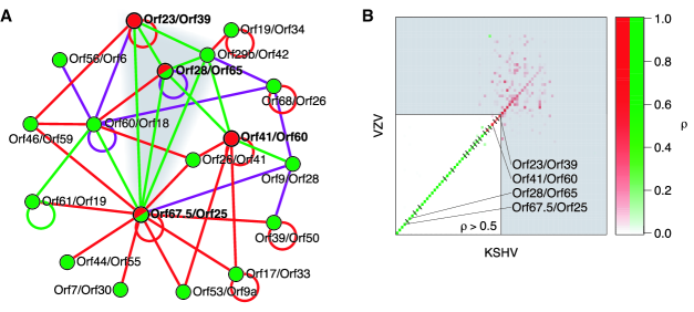
Figure 3: Alignment of the protein interaction networks of herpes viruses VZV and KSHV. a) The optimal alignment is shown with nodes representing aligned pairs of Orfs. Nodes are colour coded according to sequence similarity, measured by the sequence alignment score $\theta$ as described in the supplementary text. Green nodes have high sequence similarity with $\theta>0$, red nodes have no sequence similarity detected, red/green nodes have low similarity with $\theta\leq 0$. Protein interactions are represented by links between nodes, green links indicate interactions which have been detected in both KSHV and VZV. Interactions which have only been detected in KSHV or VZV are shown in magenta or red, respectively. The cluster of matching interactions linking nodes KSHV Orf23/VZV Orf39, 29b/42, 28/65, and 67.5/25 is highlighted.
b) The probing of the ‘twilight zone’ of low and no sequence similarity by the alignment is shown in the $\rho$-plot. Orf pairs with little or no sequence similarity are aligned due to their matching interactions (red nodes, same colour scheme as in a). The conservative consensus alignment with $\rho>0.5$ is at the bottom left. At lower values of $\rho$ spurious alignments occur (top right, see Methods). The marked cases yield functional predictions discussed in the text.

The quality of the alignment we have obtained can be tested by comparing the genomic positions of the aligned Orfs. We count the ranks of Orfs from the initial terminal repeats of the two genomes (left TR of KSHV, TRL of VZV). In Figure 4(a) the ranks of reading frames in VZV are plotted against the ranks of their alignment partners in KSHV. Aligned Orfs without any sequence similarity fit very well into the sequence of Orfs in their respective genomes. In addition, the molecular weights of the aligned nodes are highly correlated, see Figure 4(b).

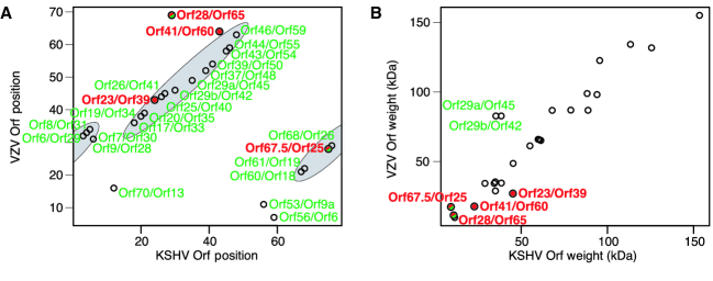
Figure 4: Corroborating evidence for the network alignment from gene position and molecular weight. a) The gene rank of reading frames of VZV is plotted against the rank in KSHV of their alignment partner. The points fall into two diagonal bands indicating the conservation of gene order between the two viruses. The Orf pairs aligned solely on the basis of matching interactions fall within the those bands. The only significant deviation from those bands, the pair KSHV Orf28/VZV Orf65, has related sequences, see text.
b) The molecular weights of aligned pairs of reading frames show a strong correlation (Pearson’s correlation coefficient $r=0.94$). The two exceptions again are aligned because they have related sequences (top left, indicated in green). The aligned Orfs with little or no sequence similarity (red circles, see text) show highly correlated molecular weights.

In some cases, sequence similar pairs of Orfs are not aligned because of mismatched interactions. As an extreme case an Orf may have several interactions in one species, but none in the other, indicating most likely an unsuccessful Y2H experiment. Examples are KSHV Orf64/VZV Orf22, 22/37, 42/53, 36/47, and 33/44.

Functional relationships detected by interaction similarity. Some Orfs are aligned due to their matching interactions, either with low or with no detectable sequence similarity. We discuss these cases separately.

KSHV Orf67.5/VZV Orf25. These Orfs have a sequence identity of only $18\%$ over $76$ aa (see Methods for details). They are listed as homologs in the VIDA3 database [20], and both of them are thought to be homologs of the HHV-1 protein U_L33 [21]. The alignment of these Orfs largely results from $4$ matching links out of $5$ in KSHV and $12$ in VZV (p-value of $4\times 10^{-3}$, see supplementary text for details) with a local link score $S_{L}=4.57$ versus node score $S_{N}=4.20$. Our alignment thus confirms the homology.

KSHV Orf28/VZV Orf65. These Orfs have a sequence identity of only $11\%$ over 102 aa. They are not listed as sequence homologs in databases VOCS [14], VIDA3 [20] and NCBI [15]. However, the sequence alignment extends over their complete length, with no gaps. Again, the alignment of these nodes results from $4$ matching links out of $4$ in KSHV and out of $5$ in VZV (p-value of $10^{-3}$) with a local link score $S_{L}=6.30$ versus node score $S_{N}=3.50$. Functional annotation is available only for VZV Orf65; it belongs to the membrane/glycoprotein class, most likely it is a type-II membrane protein [22]. The alignment of KSHV Orf28 with VZV Orf65 leads us to predict that KSHV Orf28 also codes for a membrane glycoprotein.

Several experimental studies support this prediction. Gene expression studies show that Orf28 is co-expressed with tertiary lytic Orfs and hence probably falls in the classes of structural or host–virus-interaction genes [23, 24]. The expression of Orf28 is affected by blocking DNA replication [25] showing Orf28 is a secondary or tertiary gene. Furthermore, Orf28 has been detected in the virion by mass spectroscopy, leading to a tentative functional classification as a glycoprotein–envelope protein [26]. Finally, Orf28 is a positional homolog of the Epstein-Barr virus Orf BDLF3, which is known to encode glycoprotein gp150.

KSHV Orf23/VZV Orf39. These Orfs have no significant sequence similarity: although the alignment obtained with clustalW [27] has a sequence identity of $18\%$ over $240$ aa, it is statistically insignificant; a randomised test yields a p-value of $0.43$. A systematic analysis involving a wide range of different scoring parameters does not yield a statistically significant sequence alignment either (see supplementary text). The reading frames KSHV Orf23 and VZV Orf39 are aligned purely due to $3$ matching interactions out of $4$ of KSHV and $4$ of VZV (p-value $2\times 10^{-2}$). The local link score equals $4.47$ versus a node score of $-0.49$. Functional classification is available only for VZV Orf39 as a membrane/glycoprotein [20]. The alignment thus leads us to predict that KSHV Orf23 also codes for a membrane glycoprotein.

This prediction is supported by several experimental studies. Again Orf23 is co-expressed with tertiary lytic Orfs [23] and is sensitive to blocked DNA replication [25], so it is a late gene. The expression patterns of Orf23 are similar to those of structural and packaging genes.

KSHV Orf41/VZV Orf60. These Orfs have $3$ matching interactions out of $3$ in KSHV and $6$ in VZV ($p=2\times 10^{-2}$), but no significant sequence similarity (The clustalW sequence alignment has identity of $12\%$ over $160$ aa with p-value $0.94$). They are aligned with a local link score of $4.39$ versus a node score of $-0.49$. Both Orfs are functionally annotated. KSHV Orf41 codes for a helicase/primase associated factor [28] and is not affected by blocking DNA replication [25]. On the other hand, VZV Orf60 codes for the glycoprotein L [20, 29]. It may be that either of them has a so-far unknown function, leading to the matching protein interactions. This idea finds support in [23], where the expression maximum of Orf41 was found to come after the secondary lytic phase. This is surprising because the transcript is needed already during the secondary lytic phase (DNA replication). No other DNA-replicating gene controlled by a different operon to KSHV Orf41 has an expression dynamics with this property. Such a delay of the maximum of expression may have two reasons: either the transcription of the Orf41 is not controlled after its role is finished, or Orf41 indeed has a hitherto uncharacterised function in the tertiary lytic phase, possibly a structural one.

We also note that Orf41 is specific to the class of $\gamma$-herpesviruses, of which KSHV is a member. Analogously, Orf60 is $\alpha$-herpesvirus specific. It is possible that the homolog of Orf41 in VZV and the homolog of Orf60 in KSHV were lost as a result of either of these proteins acquiring a new function. This would be an example of non-orthologous gene displacement [10].

Interaction clusters. The alignment shown in the Figure 3(a) contains a cluster of genes all interacting with each other. This cluster comprises the aligned pairs KSHV Orf23/VZV Orf39, 28/65, 29b/42, and 67.5/25 connected by matching links only. The p-value for such a fully connected cluster (a clique) to emerge at random is approximately $5\times 10^{-11}$. The pair KSHV Orf41/VZV Orf60 discussed above is connected to this cluster by two matching links, forming an almost fully connected cluster of $5$ Orfs pairs with $8$ of $10$ possible links present and matching. Surprisingly, while all the other Orfs in the cluster code for structural proteins (virion assembly and structure proteins), Orf41 of KSHV is annotated as a helicase/primase associated factor, and hence a gene involved in DNA replication. The association with structure-related genes may be interpreted as a further evidence towards another function of Orf41 as a structural Orf.

The individual species contain further clusters, but these are not conserved across species. The cluster comprising Orfs 28, 29b, 41 and K10 in KSHV contains genes coding for predicted virion proteins, virion assembly and host–virus interaction proteins. Orfs 25, 19, 27, and 38 forming a fully connected cluster in VZV code for proteins involved in virion assembly, nucleotide repair, metabolism, and host–virus interaction.

Discussion

Graph alignment results from sequence and interaction similarity. Our alignment of Orfs in two different herpes viruses yields a cross-species mapping between Orfs based jointly on the correlation between amino acid sequences and on the correlation between their protein interactions. This approach is distinct from searching for the overrepresentation of matching interactions among sequence homologs [30]. It allows the identification of homology in cases where sequence similarity between two Orfs has decayed to statistically insignificant levels. The resolution of this ‘twilight region’ of sequence similarity by using the information on protein interactions is particularly relevant for the case of short genes (such as in the present application), or high levels of domain shuffling. It also allows to detect functional analogs, proteins with similar interactions but without common ancestry.

Functional predictions from interaction similarity. We find several cases of Orfs with no detectable sequence similarity which are aligned with each other solely on the basis of matching interactions. There are different possible mechanisms generating this situation; (i) a pair of orthologous genes lose their sequence similarity, and (ii) a gene functionally substitutes for another gene. The original gene may then be excised from the genome without phenotypic effect. This process has been termed non-orthologous gene displacement [10].

In both of these cases, sequence information is insufficient for functional prediction. Based on the alignment due to matching interactions and on the annotation of one of the alignment partners, we predict the function of several Orfs. These predictions are supported by gene expression experiments and by the genomic position of the Orfs.

Functional cluster as conserved subgraph. The optimal alignment (Figure 3(a)) contains a cluster of $4$ Orfs whose products all interact with each other in both viruses. All members of this cluster belong to a single functional class; they are involved in virion formation and structure and code for tertiary lytic transcripts.

There are other fully connected clusters both in VZV and KSHV, but none of them occur in both viruses. These clusters contain proteins in different functional classes; one cluster in VZV contains proteins involved in virion assembly, nucleotide repair, metabolism, and host–virus interaction.

The guilt-by-association scheme of assigning like functions to interacting proteins [31] would fail in these cases. Refinement of the principle to guilt-by-conserved-association, where functional correlation is only assumed for proteins with an interaction in both species, correctly describes the functional correlations in the above clusters. Looking at the functions of interacting genes in a single species, the functional classes are only correlated very weakly (mutual information entropy of $0.006$ bits, see supplementary text). However, pairs of proteins with conserved interactions are more likely to share the same function (mutual information entropy of $0.107$ bits).

Guilt-by-conserved-association might go beyond the statistical significance gained from filtering false positives by cross-species comparison. Interactions between proteins of the same functional class are $1.6$ times as likely to be conserved between VZV and KSHV than interactions between proteins of different functions. Correspondingly, the mutual information on links between homologous pairs of Orfs is nearly ten times higher for Orfs of the same function than for Orfs of different function. This points to a particular mode of evolution of protein interactions, namely interactions between proteins of like function changing more slowly than those between proteins of different function. Multi-species alignments of interactions networks will provide an opportunity to address evolutionary questions of this type by tracing the dynamics of interactions along the phylogenetic tree.

Data deposition: The protein interactions for KSHV strain BC-1 and VZV Oka-parental were taken from the yeast two-hybrid screens (Y2H) of the Peter Uetz lab [4]. The sequences of the two herpesviruses were downloaded from the VOCs database [14] and the NCBI database [15, 16, 17].

Accession numbers: Genomes: KSHV: Human herpesvirus 8 strain cell line BC-1 (VOCs genome ID 890); VZV: Human herpesvirus 3 strain Oka parental (VOCs genome ID 921). KSHV Orfs: Orf 67.5: provided by Peter Uetz, sequence follows: ”MEYASDQLLP RDMQILFPTI YCRLNAINYC QYLKTFLVQR AQPAACDHTL VLESKVDTVR QVLRKIVSTD AVFSEARARP”; Orf 28: Genbank accession NP_572080.1; Orf 23: NP_572075.1; Orf 41: NP_572094.1; Orf 29b: NP_572081.1. VZV Orfs: Orf25: VOCs ID 59436; Orf65: 59475; Orf39: 59450; Orf60: 59470; Orf42: 59453.

Acknowledgments: The authors thank Peter Uetz for several fruitful discussions and making the interaction data available prior to publication, Gordon Brown and Derek Gatherer for discussions on the protein sequence alignment, and Maria Mar Albà for providing functional information data. Funding from the DFG is acknowledged under grants SFB 680, SFB-TR12, and BE 2478/2-1. This research was supported in part by the National Science Foundation under Grant No. PHY05-51164

Supplemental Text

1 Networks comparison

1.1 Protein interaction networks data

The protein interaction data comes from the work of the group of Peter Uetz, [1], and is publicly available as the supplement of the cited article.

1.2 Network alignment

The protein interaction data are represented by a network (a graph) in which each nodes represents an Orf of a species, and links denote experimentally observed protein interactions. The two herpesviral protein interaction networks are shown in the Figure 5. We denote the KSHV network as $A$ and the VZV network as $B$ when applicable. The networks $A$ and $B$ are described by their adjacency matrices, which are square matrices with terms $a_{ij}$, $b_{ij}$ equal $1$ if there is a link between Orfs $i$ and $j$ in the respective interaction network and zero otherwise.

A network alignment of two networks is a one-to-one mapping $\pi$ from the set of nodes (Orfs) of the network $A$ to the set of nodes of the network $B$:

$$\pi:\{i\in A\}\to\{j\in B\},\quad j=\pi(i).$$ (1)

The nodes that are not aligned to any node in the other species, are in our implementation aligned to a virtual dummy node.

Each network alignment may be assessed by a score combining both interaction and sequence data. The score we define in the following text is a log-likelihood score that stems from the comparison of two models: a model of evolutionary related networks and the null model of independently created nodes and links. The score has two parts; the first contribution to the alignment score quantifies the similarity of interactions of the aligned Orfs that is the local topological likeness of the two networks. Hence it is connected with the links of the networks and we term it the link score $S_{L}$. The other part utilises the sequence similarity of aligned Orfs, and hence it is connected with the nodes. We term it the node score $S_{N}$. The two contributions sum up to make the total score of the alignment

$$S=S_{L}+S_{N}.$$ (2)

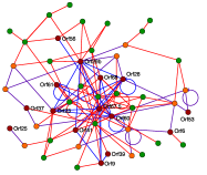
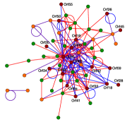
Figure 5: The protein interaction networks of a) KSHV and b) VZV. Each node in a network represents a single Orf. A link between two Orfs represents an observed protein–protein interaction. The subnetworks that belong to the final alignment are shown by dark red nodes and blue links. Their nodes are distributed homogeneously in the networks. The orange nodes are the Orfs that have been pruned out during the alignment pruning. Together with dark red nodes they show position of the consensus alignment. The violet links belong to the consensus alignment. All other nodes are plotted green and the links red.

1.2.1 Link score

The alignment of nodes induces an alignment of links; a link present between two nodes in one network may either be present or absent between their alignment partners in the other network. The topological part of the score is expressed as a sum of all rewards for aligned links that are present in both networks (matching links, conserved links) and of all penalties for the links that are present in one network only (mismatching links). These rewards/penalties are parameterised by scoring matrices $s_{l}$ for links between different nodes and $s_{s}$ for self-links. If we denote by $A^{\pi}$ and $B^{\pi}$ the subnetworks of the networks $A$ and $B$ that are aligned, that is the sets of nodes that have alignment partners together with all links within these sets, we may write the total link score as

$$S_{L}(\pi)=\sum_{(ij)\in A^{\pi}}s_{l}(a_{ij},b_{\pi(i)\pi(j)})+\sum_{i\in A^{\pi}}s_{s}(a_{ii},b_{\pi(i)\pi(i)})\ ,$$ (3)

where $\pi(i)$ is the alignment partner of the node $i\in A$ in the network $B$.

The parameters $s_{l}$ and $s_{s}$ are inferred by comparison of the model of evolutionarily related networks and of the null hypothesis in which the networks evolved independently. While in the independently evolved networks the existence of links between nodes $i,i^{\prime}$ and $j=\pi(i),j^{\prime}=\pi(i^{\prime})$ are uncorrelated, the existence of links between homologous genes in the two evolutionarily related networks will correlate. The extend of this correlation, which depends on the evolutionary distance of the two networks, specifies the magnitude of the scoring parameters $s_{l}$ and $s_{s}$. We infer their values from the available protein–interaction data in the Section 1.2.4.

1.2.2 Node score

In general, we expect that evolutionary related Orfs have correlated sequences and hence we want to reward the alignment of nodes with correlated sequences and penalise the alignment of pairs of nodes with dissimilar sequences. The measure of the similarity of the sequences is the score $\theta$ of the sequence alignment which will be thoroughly defined in the Section 2. The node score is then parameterised by some function $s_{1}(\theta)$, which is to be inferred from the data and which we expect to be an increasing function of $\theta$. Similarly, we also want to penalise the existence of pairs of Orfs that are not aligned but have similar sequences. We expect the scoring function $s_{2}(\theta)$ which parameterises this contribution to the node score. Again this function needs to be inferred from the data and is expected to be a decreasing function of the sequence similarity $\theta$.

Both functions $s_{1}$ and $s_{2}$ express the differences between the evolutionarily related networks and the model of independently evolved networks. In the evolutionary model, we expect that homologous genes, that is genes with high sequence similarity $\theta$, are aligned. In the model of unrelated networks, we expect on the contrary, that the potentially aligned genes are not similar in their sequences. We expect also that in the evolutionarily model no pair of Orfs that are not aligned has high sequence similarity. Thus when compared to the unrelated networks of the null model, the frequency of such highly sequence similar pairs must be lower. The parameter functions $s_{1}$ and $s_{2}$ gauge the difference of the evolutionarily and unrelated–networks model and are inferred from the sequence and protein interaction data in the Section 1.2.6. The total node score is expressed as

$$S_{N}(s_{1},s_{2},\pi)=\sum_{i\in A^{\pi}}s_{1}(\theta_{i\pi(i)})+\sum_{\mathrm{others}}s_{2}(\theta_{jk})\ ,$$ (4)

where we first sum all the rewards/penalties for the aligned pairs and then we add the contributions of all the pairs that are not aligned to each other but at least one Orf of the pair is aligned to some partner. The two symbolic sums may be rewritten for any alignment $\pi$ as

$$S_{N}(s_{1},s_{2},\pi)=\sum_{i\in A^{\pi}}\left[s_{1}(\theta_{i\pi(i)})+\sum_{j\in B\setminus\pi(i)}w^{\pi}_{ij}s_{2}(\theta_{ij})+\sum_{j\in A\setminus i}w^{\pi}_{j\pi(i)}s_{2}(\theta_{j\pi(i)})\right],$$ (5)

where $A\setminus i$ is the set of all nodes in $A$ but $i$ and the factor $w^{\pi}_{ij}$ prevents overcounting of score contributions. Its value is $1$, when only one of $i$ and $j$ is aligned, and $0.5$ when both nodes are aligned to different partners.

1.2.3 Matrix representation of the score and the difference algorithm

The problem of finding the optimal network alignment is mapped to the quadratic assignment problem, which is solved iteratively by repeated solutions of the Linear Assignment Problem.

Both contributions to the alignment score, link and node score, can be expressed in a matrix form. The node score is encoded in the matrix $M^{\pi}$ and the topological part of the score in the matrix $R^{\pi}$:

$$S=S_{N}+S_{L}=\mathrm{Tr}\;\pi(M^{\pi}+R^{\pi})\ ,$$ (6)

with

$$M_{ij}^{\pi}=\frac{1}{2}\sum_{k\in A^{\pi},k\neq j,\pi(k)\neq i}s_{l}(a_{jk},b_{i\pi(k)})+s_{s}(a_{jj},b_{ii})\ ,$$ (7)

and

$$R_{ij}^{\pi}=s_{1}(\theta_{ji})+\sum_{k\in B\setminus i}w^{\pi}_{jk}s_{2}(\theta_{jk})+\sum_{k\in A\setminus j}w^{\pi}_{ki}s_{2}(\theta_{ki})\ .$$ (8)

$\mathrm{Tr}M$ stands for the trace of matrix $M$.

For the sake of algorithm performance, we use instead of the total score its generalised derivative, that is the change of the score upon addition or removal of a node pair $ji$ to the alignment. This approach makes the algorithm more greedy during the initial phase, yet keeps it exact in the final stage. The derivative as represented in a matrix form reads

$$\Delta M_{ij}^{\pi}=\sum_{k\in A^{\pi},k\neq j,\pi(k)\neq i}s_{l}(a_{jk},b_{i\pi(k)})+s_{s}(a_{jj},b_{ii})$$ (9)

for the change of the node score and

$$\Delta R_{ij}^{\pi}=s_{1}(\theta_{ji})+\sum_{m\in B\setminus B^{\pi},m\neq i}s_{2}(\theta_{jm})+\sum_{m\in A\setminus A^{\pi},m\neq j}s_{2}(\theta_{mi})\ .$$ (10)

for the change of the link score. The iterative update of the alignment is then done according to the scoring matrix $\Delta M^{\pi}+\Delta R^{\pi}$, by repeatedly solving the linear–assignment problem instance, [4].

$$\pi\leftarrow\mathrm{argmax}_{\pi^{\prime}}\mathrm{Tr}\;\pi^{\prime}(\Delta M^{\pi}+\Delta R^{\pi}+T\chi\eta)$$ (11)

until convergence. A noise term has been added so the algorithm can escape from local score maxima: $\eta$ is a random matrix with terms drawn independently at each iteration from the normal distribution with the mean 0 and the standard deviation 1. The addition of this random matrix similar to the simulated annealing method of statistical physics, [5]. The amplitude of the noise starts at an initial value $T$ and decreases continuously; the schedule function $\chi$ is a linear function decreasing from 1 at the beginning of the algorithm run to 0 at its end. The temperature $T$ specifies the depth valleys in the score landscape the algorithm can overcome and hence extent of the space of alignments that is sampled. The higher the temperature $T$, the larger the volume of the space of alignments that is sampled.

A package called GraphAlignment implementing this algorithm under the R-project is available for download on [6].

1.2.4 Score parameters

In order to find the score parameters, we evaluate the likelihood of the scenario in which the two networks evolved from a common ancestor and compare it to the likelihood of the null model of two independently created ER networks.

The likelihood of an alignment $\pi$ of the interaction networks $A$ and $B$ reads

$$P(\pi|\{A,B\})=\frac{P(\{A,B\}|\pi)P(\pi)}{P(\{A,B\})}\ ,$$ (12)

where, within the Viterbi approximation [7], the prior $P(\{A,B\})$ consists of the two terms in comparison: the evolutionarily related model ($\pi$) and the null hypothesis ($R$).

$$P(\{A,B\})=P(\{A,B\}|\pi)P(\pi)+P(\{A,B\}|R)P(R)\ .$$ (13)

The likelihood may be expressed in terms of a log-likelihood score $S$ in the form of the sum of the link and node score $S=S_{L}+S_{N}$, (2),

$$P(\pi|\{A,B\})=\frac{1}{1+e^{-S(\pi)}}\ .$$ (14)

This score consists of two independent terms: The contribution depending on the network topology in the conditional probabilities $P(\{A,B\}|\pi)$ and $P(\{A,B\}|R)$, and the contribution of the priors $P(\pi)$ and $P(R)$. The independence of the two terms allows us to assign the topological score $S_{L}$ to the first one and the node score $S_{N}$ to the latter term,

$$S_{L} = \ln\frac{P(\{A,B\}|\pi)}{P(\{A,B\}|R)},$$ (15)

$$S_{N} = \ln\frac{P(\pi)}{P(R)}.$$

By identifying (15) with (3, 4) we can readily find the scoring matrices $s_{s}$ and $s_{l}$ together with the scoring functions $s_{1}$ and $s_{2}$. Before doing so, we introduce a new quantity, the density matrix, which allows us to control closely the behaviour of the aligning algorithm.

1.2.5 Density matrix $\rho$

For the evaluation of the scoring parameters we accumulate the results of several runs of the alignment algorithm.

To store this data, we define the density matrix $\rho$ in the following way. We count the number of times $m_{ij}$ a pair of nodes $i\in A$ and $j\in B$ were aligned in $M$ runs of the algorithm, and set the corresponding matrix term $\rho_{ij}=m_{ij}/M$. We can rewrite the definition in terms of the resulting alignments $\pi^{\alpha}$,

$$\rho_{ij}=\frac{1}{M}\sum_{\alpha=1}^{M}\delta(\pi^{\alpha}(i),j)\ .$$ (16)

By $\pi^{\alpha}(i)$ we denote the alignment partner of the node $i\in A$ in the graph $B$ in the run $\alpha$. The term $\rho_{ij}$ of the density matrix then approximates the probability of finding the pair $(ij)$ in the final alignment.

1.2.6 Mean values of the scoring parameters

For the evaluation of the link score matrices we count frequencies matched/mismatched links in the alignment. That is, for each pair $(i,i^{\prime})\in A$ and the alignment partners $j=\pi(i)$ and $j^{\prime}=\pi(i^{\prime})$ the terms $a_{ii^{\prime}}$ and $b_{jj^{\prime}}$ of the entries of the adjacency matrices are compared and the frequency table is accordingly updated. We calculate the frequency tables both for the links and the self-links:

$$q_{l}(a,b) = \frac{1}{N_{l}}\sum_{(i,j)\in A}\sum_{(k,l)\in B}\rho_{ik}\rho_{jl}\delta({a_{ij},a})\delta({b_{kl},b}),$$ (17)

$$q_{s}(a,b) = \frac{1}{N_{s}}\sum_{i\in A}\sum_{k\in B}\rho_{ik}\delta({a_{ii},a})\delta({b_{kk},b})\ ,$$

where $N_{l}$ and $N_{s}$ are the normalisation constants of the two distributions and $a,b\in\{0,1\}$.

If the two networks evolved independently, as it is assumed in the null model, we can marginalise the frequency tables and find the probabilities of having a link between two nodes in the graph $A$ or $B$,

$$p_{l}^{A}(a) = \sum_{b=0}^{1}q_{l}(a,b),$$ (18)

$$p_{l}^{B}(b) = \sum_{a=0}^{1}q_{l}(a,b).$$

By the marginalisation of the self link distribution, we obtain $p_{s}^{A}$ and $p_{s}^{B}$.

Finally, we obtain the score parameters $s_{l}$ and $s_{s}$ by comparing the null and evolutionary model,

$$s_{r}(a,b)=\ln\frac{q_{r}(a,b)}{p_{r}^{A}(a)p_{r}^{B}(b)},\quad r\in\{l,s\}.$$ (20)

Similarly, the node score parameters are inferred from the sequence similarities $\theta_{ij}$ and the current alignment. Three situations may occur for a pair of Orfs $i\in A$ and $j\in B$. Either the two Orfs are aligned in $\pi$, or they are aligned to some other partners, but not to each other, or they are not aligned to any partner. These three disjoint sets of pairs of Orfs define three ensembles for which we evaluate frequencies of the sequence similarity $\theta$; $d_{1}(\theta)$ for the aligned pairs, $d_{2}(\theta)$ for the second ensemble, and $d_{0}(\theta)$ for the pairs of nodes that are not aligned. We take the score $\theta$ as defined in the Section 2 as the sequence similarity measure. The three distributions of $\theta$ are

$$d_{1}(\theta) = \frac{1}{N_{1}}\sum_{i\in A}\sum_{j\in B}\rho_{ij}\theta_{ij},$$ (21)

$$d_{2}(\theta) = \frac{1}{N_{2}}\sum_{i\in A}\sum_{j\in B}(1-\rho_{ij})\left[1-\prod_{k\in A,k\neq i}(1-\rho_{kj})\prod_{l\in B,l\neq j}(1-\rho_{il})\right]\theta_{ij},$$ (22)

$$d_{0}(\theta) = \frac{1}{N_{0}}\sum_{i\in A}\sum_{j\in B}(1-\rho_{ij})\prod_{k\in A,k\neq i}(1-\rho_{kj})\prod_{l\in B,l\neq j}(1-\rho_{il})\theta_{ij}\ ,$$ (23)

where $N_{0}$, $N_{1}$, and $N_{2}$ are normalisation constants. In general, we expect $d_{1}(\theta)$ to be an increasing function of $\theta$, reflecting the fact that the aligned Orfs should have similar functions. Indeed, many sequence–homologous pairs belong to this set. The distribution $d_{2}(\theta)$ is, on the other hand, expected to be a decreasing function of $\theta$, similarly to $d_{0}(\theta)$.

The distribution $d_{0}(\theta)$ of similarities of unaligned Orfs may be considered as the background distribution of $\theta$, and is taken as the distribution in the null model. The node scores $s_{1}$ and $s_{2}$ read

$$s_{r}(\theta)=\ln\frac{d_{r}(\theta)}{d_{0}(\theta)},\quad r\in\{1,2\}.$$ (24)

1.2.7 Consensus and pruned alignment

From the $\rho$ matrix we extract the consensus alignment as the alignment of Orfs that have the corresponding $\rho$-matrix term larger than $0.5$. This conservative choice of the cut-off is further discussed in the following section.

The consensus alignment is then pruned in order to remove marginally aligned pairs. These we define as the pairs that have a negative sequence score and at the same time less than two matching interactions. This pruning removes spuriously aligned pairs with both low sequence similarity and low topological match.

1.2.8 Estimate of the p-value of the network alignment

To calculate the p-value of aligning two nodes $i\in A$ and $j\in B$, we remove the pair $(ij)$ from the alignment and find the probability of placing in the vacancy a pair of nodes with a topological match as good or better than the match of the pair $(ij)$. These two nodes are chosen from two ER networks with sizes and mean connectivities identical to those of the KSHV and VZV networks. These two unrelated ER graphs correspond to the null model of independently evolved networks.

A pair of nodes has the same or better topological match whenever it has the same or a larger number of matching links to other aligned pairs or it has a smaller number of mismatching links. For the pair $(ij)$ with $r$ matching links in the alignment graph (Figure 3a in the main text) the p-value is defined as the probability of finding a nodes pair with $r$ or more matching links and at most $n_{A}-r$ (resp. $n_{B}-r$) mismatching links, where $n_{A}$ ($n_{B}$) is the total number of links adjacent to $i$ in $A^{\pi}$ ($j$ in $B^{\pi}$).

This probability is easily evaluated for uncorrelated networks using the multinomial distribution. For $p_{A}\ll 1$ and $p_{B}\ll 1$ it reads

$$\!\!\!\!\!\!\!\!\!\!\!\!\!\!p(r,n_{A},n_{B},N^{\pi})=$$ (25)

$$(N_{A}-N^{\pi}+1)(N_{B}-N^{\pi}+1)$$

$$\times\;\;\sum_{m_{A}=r}^{n_{A}}\sum_{m_{B}=r}^{n_{B}}\sum_{s=r}^{s=\min\{m_{A},m_{B}\}}\begin{pmatrix}N^{\pi}-1\\ s,m_{A}-s,m_{B}-s,N^{\pi}-1-m_{A}-m_{B}+s\end{pmatrix}$$

$$\times\;\;[p_{A}p_{B}]^{s}[p_{A}(1-p_{B})]^{m_{A}-s}[(1-p_{A})p_{B}]^{m_{B}-s}[(1-p_{A})(1-p_{B})]^{N^{\pi}-1-m_{A}-m_{B}+s}\ ,$$

where $N^{\pi}$ is the size of the aligned subnetworks ($N^{\pi}=26$), and $p_{A}$ and $p_{B}$ are the link probabilities in the two ER graphs which we estimate from the complete KSHV and VZV networks respectively, giving $p_{A}=0.0330$ and $p_{B}=0.0561$. The individual terms of equation (25) can be understood intuitively: first we choose a node in the network $A\setminus A^{\pi}\cup i$ (one node out of $N_{A}-N^{\pi}+1$), and a partner node from the network $B\setminus B^{\pi}\cup j$. Next we choose from the $N^{\pi}-1$ remaining nodes in the alignment network $s$ nodes that are connected by matching links with the probability $p_{A}p_{B}$, $m_{A}-s$ (resp. $m_{B}-s$) nodes that are connected by links only in the KSHV (VZV) subnetwork with appropriate probability, and the remaining nodes that are not linked to the pair $(ij)$ in either subnetwork. Finally, we sum over all possible choices of the nodes (the multinomial coefficient) and over all options that are equally good or better than the actual alignment of $(ij)$. The contribution from the self–links (which are typically mismatching) is close but smaller than $1$ and is neglected here. The result is then an upper bound of the p-value. The estimated p-values for the pairs of Orfs discussed in the main text are listed in the Table 4.

Similarly, we estimate the p-value of finding in the alignment networks a clique with $M_{C}$ pairs, out of which $M_{O}$ pairs are sequence related, and which are connected by matching links only. We calculate this p-value as the probability of finding such a clique and of finding among the links adjacent to the vertices of the clique the same number or more matching links and the same number or less of links that are present in one PIN only. Denoting the pairs of the clique $(i^{a}j^{a})$, where $a\in\{1,2,\ldots,M_{C}-M_{O}\}$, the numbers of the matching links $r^{a}$, and the total number of links adjacent to $i^{a}$ ($j^{a}$) in KSHV (VZV) as $n_{A}^{a}$ ($n_{B}^{a}$), this p-value is

$$\!\!\!\!\!\!\!\!\!\!\!\!\!\!p(M_{C},M_{O},\{r^{a}\},\{n_{A}^{a}\},\{n_{B}^{a}\},N^{\pi})=$$ (26)

$$\begin{pmatrix}N_{A}-N^{\pi}+M_{C}-M_{O}\\ M_{C}-M_{O}\end{pmatrix}\begin{pmatrix}N_{B}-N^{\pi}+M_{C}-M_{O}\\ M_{C}-M_{O}\end{pmatrix}(M_{C}-M_{O})!(p_{A}p_{B})^{M_{C}\choose 2}$$

$$\times\prod_{a=1}^{M_{C}-M_{O}}\sum_{m_{A}=r^{a}}^{n_{A}^{a}}\sum_{m_{B}=r^{a}}^{n_{B}^{a}}\!\!\!\sum_{s=r^{a}}^{s=\min\{m_{A},m_{B}\}}\begin{pmatrix}N^{\pi}-M_{C}\\ s,m_{A}-s,m_{B}-s,N^{\pi}-M_{C}-m_{A}-m_{B}+s\end{pmatrix}$$

$$\times\;\;[p_{A}p_{B}]^{s}[p_{A}(1-p_{B})]^{m_{A}-s}[(1-p_{A})p_{B}]^{m_{B}-s}[(1-p_{A})(1-p_{B})]^{N^{\pi}-M_{C}-m_{A}-m_{B}+s}\ .$$

The contribution of self links is again omitted and giving upper bound to the p-value. The formula (26) reduces to (25) in the case of an isolated node (1-clique) in which case $M_{C}=1,M_{O}=0$.

The p-value for the clique formed by the pairs $67.5/25$, $28/65$, $29b/42$, $23/39$ given by (26) is $5\times 10^{-11}$. The p-values of finding such a clique in the PINs of the two species can be estimated similarly and they are $2\times 10^{-3}$ in KSHV and $4\times 10^{-2}$ in VZV. The difference between the p-value inferred from the aligned networks and the p-values estimated from the single–species networks indicates the significance of the evolutionary conservation of the clique.

1.3 Test of the procedure on artificial data

We test the performance of the algorithm on artificially generated networks with topological characteristics similar to those of the actual KSHV and VZV networks. Since the correct alignment is known for the generated networks, we can assess the specificity and selectivity of the graph alignment in these cases.

1.3.1 High similarity of graphs

We align two highly similar ER networks generated in the following way. An ER network is generated with $98$ links and $80$ nodes. A copy of this network is made and another $42$ links are placed in each network independently of each other. For $60$ nodes chosen at random in one of the networks, we assigned node similarity with their “orthologs”.

The two resulting networks thus share 98 links out of 140 and contain 60 sequence–homologous Orfs out of 80. With such a high similarity we expect the algorithm to find easily the correct alignment of the two networks, which is also what we observe (93% of the nodes are correctly aligned, none is misaligned, see the Figure 6). The quality of the alignment does not depend on the details of the algorithm schedule, the updating of all scoring parameters by the means of (20) and (24) is possible. With increasing temperature, the number of aligned pairs increases, yet the quality of the alignment is not compromised. The optimal performance of the algorithm is reached at an intermediate temperature $T=6$.

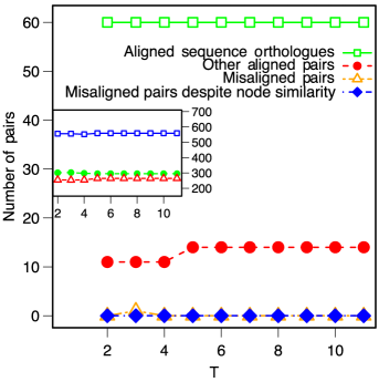
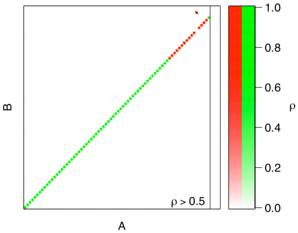
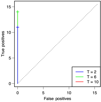
Figure 6: Alignment of two highly similar Erdős-Rényi graphs.
a) Main figure: Low noise level leads to sub-optimal alignments. The dependence of the number of aligned sequence–homologous pairs ($\square$), the number of other aligned pairs ($\circ$), the number of wrongly aligned pairs ($\triangle$), and of the number of wrongly aligned pairs in which one or both partners are sequence homologous to a different Orf ($\diamond$) on the temperature $T$.
a) Inset: For highly similar networks the score parameters are stable with updating. The resulting total ($\square$), node ($\circ$), and link ($\triangle$) scores do not vary with the temperature.
b) At $T=6$ is the alignment of the two random networks perfectly recovered. The $\rho$ matrix gives the probability of aligning nodes pairs from the networks $A$ and $B$. The Orfs $i\in A$ are sorted with decreasing value of $\max_{j\in B}\rho_{ij}$. The Orfs of $B$ are on the other hand sorted in such a way that the diagonal of the density matrix corresponds to the correctly aligned pairs and the off-diagonal elements correspond to false positive predictions. The pairs of Orfs with detectable sequence similarity are shown in green, those with no sequence similarity in red. All pairs to the left of the vertical line denoting the $50\%$ cut-off belong to the consensus alignment. The pairs that have been pruned out in the pruned alignment are crossed out.
c) Another signature of the quality of the alignment are the numbers of true and false positives. The numbers of true and false predictions are plotted and the cut-off value of $50\%$ is shown by the crosses. Only node pairs that do not have any sequence similarity are counted as true and false positives, hence the curve shows the result coming from the topological similarity only. The number of correctly aligned values increases with the temperature and reaches its optimal value at $T=6$.

1.3.2 Moderate similarity of graphs

To test the performance of the algorithm in the regime appropriate to the actual data, we repeat the test over graphs generated to resemble the data. We generated a pair of ER graphs that out of $80$ nodes and $140$ links share $49$ links and contain $32$ nodes with related sequences, and hence their level of similarity is comparable to the estimate for the real data. For these graphs we observe a nontrivial dependence of the number of aligned and misaligned pairs on the temperature; the choice of the temperature becomes crucial at this level of network conservation. As the optimal temperature we have chosen, in a conservative scheme, the largest temperature for which the values of the score parameters remain close to their values inferred from the initial alignment of sequence homologs, see Figure 7.

We observe that with decreased similarity of the two networks, the optimal temperature at which we run the algorithm decreases to some intermediate value. Already in the case of highly similar graphs we saw that the temperature must not be too low, for otherwise the sampled region of the alignment space is too small. In the example of moderately related networks we see another phenomenon: also too high a temperature decreases the quality of the alignment. The case of high temperatures is termed the low-fidelity regime, where the link score contribution grows quickly with temperature and the node score, and hence the contribution from the sequence similarity, decreases steeply. The essence of the phenomenon is best described with a very simple example of aligning two Cayley trees. If we distribute over the trees “sequence homologs” densely, the correct alignment will be recovered, as in the case of the highly similar Erdős–Rényi graphs. However, if we distribute the sequence homologs sparsely or we do not place any homologs at all in the trees, the number of possible alignments with perfectly matching links would be huge, but none of these alignments would express the actual correlation of the graphs. There would be no statistical significance of the huge score. Updating of scores according to (20) and (24) would result in a low or negligible node score and a high link score, and consequently in a low reward for aligning sequence related Orfs and an exaggerated reward for matching links. This is exactly the behaviour that is observed in the Figure 7a.

To prevent the divergence of the scoring parameters we do not update the link score parameters, instead we fix them to the values inferred from the initial alignment of sequence homologs. Furthermore, being rather conservative, we keep the temperature low, below the transition value $T_{D}$, in order to restrict the search for alignments only within the neighbourhood of the initial alignment in the configuration space. By such a restriction, we recover some of the nodes pairs properly even at low network similarity and at the same time we keep the false positives rate low, see the Figure 7b. At temperature $T=5$, that is slightly below the critical temperature $T_{D}$, we correctly recover all $32$ sequence homologs, and another $5$ pairs of Orfs without sequence similarity. In total, we recover $46\%$ of the complete network with $80$ nodes. If we concentrate on the orthologs without sequence similarity solely, the algorithm recovers at $T=5$ $10\%$ of non-sequence homologous pairs. Here we note that among non-sequence homologous pairs only $73\%$ have some topological similarity, $33\%$ share at least two links, and only $10\%$ share three or more links. The aligned pairs without sequence similarity share two or three links.

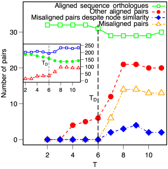
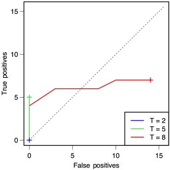
Figure 7: Alignment of two moderately related Erdős-Rényi graphs. For the legend see the caption of the Figure 6. See also the Figure 2 in the main text for the corresponding $\rho$-matrix.
a) Low-fidelity regime is linked to a steep increase of the link score. Inset: The low-fidelity alignments have scores higher than the alignment of the sequence homologs, hence the search must be restricted only to the alignments in the vicinity of the sequence–homologs alignment. The temperature $T_{D}$ manifests itself in the steep increase of the link score.
b) Intermediate values of $T$ are optimal for searching the optimal alignment. The false–true positives curves show that for too low $T$ the recovered alignment is trivial, and for too high $T$ it is faulty. The intermediate temperature $T=5,T\lesssim T_{D}$, shows the best ratio of true positives.

2 Sequences comparison

2.1 Genome data

The sequences of the two herpesviruses (KSHV strain BC-1 and VZV Oka-parental) have been downloaded from the VOCs database [3]. Further Orfs (alternative splices) have been obtained from the NCBI database [8] or the VIDA database [2] or have been provided by Peter Uetz [1].

2.2 Sequence alignment

To assess mutual sequence similarity of the Orfs in the two viral species we generate sequence alignments of each KSHV Orf with each VZV Orf. Since the open reading frames are short and the level of sequence similarity is low, care has to be taken in obtaining the optimal alignment, as detailed below.

To account for the uneven level of sequence conservation across the genome, we optimise the scoring parameters of the Needleman–Wunsch algorithm individually for each pair of Orfs [9]. We use affine gap penalties and the scoring matrices of the BLOSUM series (BLOSUM35 to BLOSUM90, [10]). We optimise the following parameters: the gap–opening penalty, the gap–extension penalty and the evolutionary distance encoded by the BLOSUM matrices. The code for the sequence alignment, termed sequenceAlign is available upon request.

2.2.1 Score

We define a standard log-likelihood score of an alignment of two sequences by comparing a model based on evolutionary relation of the two sequences with a random model. The random model of independently evolved sequences depends only on the frequencies of amino-acids occurring in natural peptides. If we denote these frequencies by $p(a)$, where $a$ stands for an amino-acid residue and has $20$ possible values, we may write the probability of generating randomly a sequence $\mathbf{a}$ of length $L$ with a composition $\{a_{i}\}$ as

$$P(\mathbf{a})=\prod_{i=1}^{L}p(a_{i})\ .$$ (27)

The probability of generating sequences $\mathbf{a}$ and $\mathbf{b}$ under this uncorrelated model reads

$$P^{\prime}(\lambda,\mathbf{a},\mathbf{b})=P(\mathbf{a})P(\mathbf{b})=\prod_{j=1}^{L}p(a_{j})p(b_{j})\ .$$ (28)

For evolutionary related sequences, we expect a higher probability observing two equal or similar residues, which is expressed by the log-likelihood score matrices $\sigma$. Hence

$$Q^{\prime}(\lambda,\mathbf{a},\mathbf{b})=\frac{1}{Z^{\prime}(\mathbf{a},\mathbf{b})}\prod_{j=1}^{L}p(a_{j})p(b_{j})e^{\sigma(a_{j},b_{j})}\ ,$$ (29)

where $Z^{\prime}(\mathbf{a},\mathbf{b})$ is a normalisation constant

$$Z^{\prime}(\mathbf{a},\mathbf{b})=\sum_{\lambda}\prod_{j=1}^{L}p(a_{j})p(b_{j})e^{\sigma(a_{j},b_{j})}\ .$$ (30)

The construction of the scoring matrices of the BLOSUM series ascertains that the normalisation constant $Z^{\prime}$ equals $1$ for sequences with the residue frequencies $p(a)$ close to those inferred from current databases. This condition is also typically satisfied for all proteins with $100$ and more residues. The log-likelihood score of an alignment (without gaps) is then expressed as

$$\theta^{\prime}(\lambda,\mathbf{a},\mathbf{b}) = \ln\frac{Q^{\prime}(\lambda,\mathbf{a},\mathbf{b})}{P^{\prime}(\lambda,\mathbf{a},\mathbf{b})}$$

$$= \sum_{j=1}^{L}\sigma(a_{j},b_{j})-\ln Z^{\prime}(\mathbf{a},\mathbf{b})\ .$$

With the proper normalisation of $Q^{\prime}$ by $Z^{\prime}$, the score $\theta^{\prime}$ is larger than zero whenever the two sequences $\mathbf{a}$ and $\mathbf{b}$ are more likely to evolve under the evolutionary model underlying the scoring matrices in use.

To allow gaps in the global alignment we add two more parameters to the model, the gap–opening penalty $\ln\mu$ and the gap–extension penalty $\ln\nu$ (affine gaps). The score splits into two parts: the substitutions score and the gap score:

$$\theta(\lambda,\mathbf{a},\mathbf{b},\mu,\nu,\sigma) = \ln\frac{Q(\lambda,\mathbf{a},\mathbf{b})}{P(\lambda,\mathbf{a},\mathbf{b})}$$

$$= \sum_{\mathrm{aligned\;r.}\,j}\sigma(a_{j},b_{j})+\sum_{\mathrm{gaps}\,j}\left[\ln\mu+(l_{j}-1)\ln\nu\right]-\ln Z^{L}\ .$$

Here we first sum all contributions from residue substitutions and then we sum all the gap costs. The affine gap costs increase linearly with the gap length $l_{j}$.

$Z^{L}$ is the normalisation constant of the probabilities $Q$ and it depends on the length of the alignment $L$, the two sequences, the scoring matrix in use, and the gap score parameters. Since the BLOSUM score matrices are properly normalised by construction, $Z^{\prime}=1$, or

$$\sum_{a,b}p(a)p(b)e^{\sigma(a,b)}=1\ ,$$ (33)

the only contribution to $Z^{L}$ comes from the gaps. To calculate this contribution, we will consider the following Markov chain.

We start with the two sequences completely unaligned and we choose one option of: either (i) we align the two initial residues of the considered sequences (a substitution), or (ii) we align the initial residue of the second sequence with a gap, that is, we create a gap on the first sequence (a deletion), or (iii) we create a gap on the other sequence (an insertion). In this way the alignment is started and we extend it by one of the following steps: either (i) we align the residues that follow in the two sequences (a substitution), or (ii) we create the gap on the first sequence (a deletion), or (iii) we create a gap on the other sequence (an insertion). We repeat the steps (i–iii) until the last residue is aligned to a residue or to a gap. The length of the alignment $L$ is the number of the steps in the Markov chain. For this Markov chain we can calculate the normalisation constant $Z^{L}$ by a simple transfer matrix method. At each step $l$ there are three possibilities of the end state of the alignment: either the last step was a substitution, or a deletion or an insertion. Hence, we split $Z^{l}$ in three parts $Z^{l}=Z_{s}^{l}+Z_{d}^{l}+Z_{i}^{l}$ that correspond to the respective end-states. We may express the vector $Z^{l+1}=(Z^{l+1}_{s},Z^{l+1}_{d},Z^{l+1}_{i})$ at step $l+1$ of the Markov chain as a function of the vector $Z^{l}$ at the step $l$:

$$Z^{l+1}=TZ^{l},$$ (34)

where the transfer matrix $T$ reads

$$T=\begin{pmatrix}1&1&1\\ \mu&\nu&0\\ \mu&0&\nu\end{pmatrix}.$$ (35)

At the beginning of the alignment process we may start with a substitution, a deletion or an insertion and hence $Z^{0}=(1,1,1)$. The normalisation constant for an alignment of length $L$ can be readily calculated by applying the transfer matrix $L$-times on the initial vector $Z^{0}$

$$Z^{L}=T^{L}Z^{0}.$$ (36)

For long alignments the dominant contribution comes from the largest eigenvalue of the transfer matrix $\alpha$,

$$\alpha=\frac{\nu+1+\sqrt{(\nu-1)^{2}+8\mu}}{2}\ ,$$ (37)

and it reads

$$Z^{L}=\frac{(2\mu-\nu+3\alpha)}{\sqrt{(\nu-1)^{2}+8\mu}}\alpha^{L}\ .$$ (38)

Since the logarithm of the normalisation constant $\ln Z^{L}=C(\mu,\nu)+L\ln\alpha$ is extensive in the length $L$ and since $L$ is the sum of numbers of substitutions, deletions and insertions, the normalisation can be implemented as a shift of scores:

$$\theta(\lambda,\mathbf{a},\mathbf{b},\mu,\nu,\sigma) = \sum_{\mathrm{aligned\;r.}}(\sigma(a_{j},b_{j})-\ln\alpha)$$

$$+ \sum_{\mathrm{gaps}}[\ln\mu-\ln\alpha+(l_{j}-1)(\ln\nu-\ln\alpha)]-C(\mu,\nu).$$

The score defined by the last formula is properly normalised for any choice of scoring parameters $\mu,\nu$ and $\sigma$, whenever the substitution scoring matrix is normalised according to (33). The normalisation is done against all alignments of length $L$, what is an approximation of the exact normalisation evaluated by Yu and Hwa, [11], who considered all possible alignments of the two sequences. However, this approximation allows to evaluate the normalisation constant explicitly (instead of the iterative formulae of [11]) and is at the same time a very good estimate for sufficiently large negative gap penalties. The normalisation allows us to search for the optimal parameters for an alignment of any two sequences $\mathbf{a}$ by maximising the score $\theta(\lambda,\mathbf{a},\mathbf{b},\mu,\nu,\sigma)$ over arguments: the alignment $\lambda$ and the parameters $\mu,\nu,\sigma$. This maximisation is performed iteratively by the code sequenceAlign.

The final score is computed by subtracting the contribution of leading and trailing gaps. All alignments which are either too short ($6$ residues and less) or contain too many gaps (a gap opening every $6^{\mathrm{th}}$ residue on average), are disregarded as insignificant. The final score is used as the measure of the sequence similarity $\theta$ which is used, in completion to interaction data, in the network alignment. For the remaining alignments we compute also the percent identity defined as the number of identities in the alignment divided by the total number of substitutions in the alignment. Knowing the optimal alignment and its score for all pairs of nucleotide sequences, we search for the reciprocally best matching Orfs in the two species, considered bona-fide sequence homologs.

The number of sequence homologs in the KSHV/VZV genome is 34, that is approximately $40\%$ of the Orfs of each species. The list of the sequence homologs and parameters of their alignments are given in the Table 1, together with the scores calculated using clustalW (version 1.81, default parameters [12]). For the four Orfs pairs discussed in the Results section of the main text we have estimated also p-values of the clustalW alignment and we present the data in the Table 3.

Here we define the p-value of the clustalW alignment as the probability of obtaining an alignment of two random sequences with the same or higher percent identity and with a comparable length ($\pm 10\%$) as the alignment of the real protein sequences. To generate the ensemble of random sequences ($1000$ pairs) we permute the real sequences in a random fashion. In this way we keep the lengths and base compositions of the two sequences, but we remove any sequence relation. The random pairs are afterwards aligned with clustalW and the p-value is estimated from the frequencies of the percent identities.

KSHV Orf	VZV      Orf	seq. orth.	sequenceAlign identity (%)	score	clustalW       identity (%)	score
9	28	*	43.3	467	39.8	2155
70	13	*	63.7	369	61.8	1247
44	55	*	36.5	293	34.1	1431
25	40	*	29.9	281	27.0	1628
61	19	*	32.6	174	31.2	1035
60	18	*	37.4	162	37.6	676
29b	42	*	38.4	148	37.8	680
8	31	*	24.8	145	24.3	924
29b	45		41.2	123	35.3	643
46	59	*	39.9	113	43.4	560
43	54	*	24.5	89	24.5	668
6	29	*	20.1	81	20.6	790
56	6	*	30.2	51	23.3	726
7	30	*	23.6	48	22.4	548
68	26	*	20.0	34	20.7	370
29a	45		28.5	34	25.1	305
39	50	*	18.9	32	18.6	280
37	48	*	23.5	32	19.8	291
20	35	*	34.2	22	23.0	154
17	33	*	28.1	22	21.9	311
19	34	*	19.8	10	18.1	304
53	9a	*	23.8	8	28.6	76
26	41	*	14.5	4	20.3	169
67.5	25	*	20.0	0	18.4	57
28	65	*	9.9	0	10.8	-31
53	8.5		20.8	-1	26.4	57
K6	1	*	10.6	-1	11.6	-26
69	27	*	21.7	-1	16.4	126
28	8.5		20.0	-1	14.7	-41
67	24	*	14.0	-3	14.3	2
30	8.5		16.2	-4	20.8	6
72	7	*	10.2	-7	13.4	-42
52	1		13.1	-8	18.5	7
65	0	*	20.6	-9	18.2	-19
38	49	*	21.7	-9	18.0	11
72	35		6.6	-9	13.3	-38
28	1		11.9	-10	14.7	-29
53	0		13.9	-11	17.3	31
52	46		17.7	-11	19.9	27
K6	S/L		11.7	-11	20.0	5
30	9a		14.5	-11	19.5	20
53	65		6.9	-11	15.7	-17
67.5	49		7.6	-12	11.7	-31
K5	58	*	11.4	-12	12.7	-48
67.5	9a		15.4	-12	15.6	-19
38	7		11.7	-12	29.5	16
K15	65		8.1	-12	10.1	-42
16	69	*	11.5	-12	10.9	-42
16	64	*	11.5	-12	10.9	-42
67.5	7		13.9	-13	25.0	6
K8	23	*	10.7	-13	13.9	-18
K4	S/L		12.9	-13	22.3	18
K4	9a		4.7	-13	19.2	1
53	1		4.7	-14	14.2	-28
30	57		10.0	-14	17.4	-23
74	36	*	10.0	-14	12.9	-30
55	58		9.1	-14	9.6	-93

Table 1: The detected sequence homologs: We list all the pairs of putative sequence homologs detected by sequenceAlign together with the score and the percent identity returned by the code. The score and the percent identity obtained with clustalW (version 1.81, standard parameters values) are also listed. The pairs that are considered putatively sequence homologous are marked by asterisk.

3 Graph alignment of VZV and KSHV

The optimal temperature for the algorithm run has been estimated from the Figure 8. By comparison of the plot with the Figure 7 we estimate the value of the transition temperature $T_{D}=6$ and run the alignment algorithm with the schedule defined by $T=5$. In this way, we maximise the number of aligned pairs while aiming to keep the estimated number of wrongly aligned pairs negligible. The alignment contains $26$ node pairs out $84$ of KSHV and $76$ of VZV (approximately $33\%$).

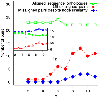
Figure 8: Choice of the temperature $T$ for the real data. For the legend see Figure 7. Main figure: The numbers of aligned pairs of the two herpesviral protein interaction networks show similar trends as in the tests with artificial data. The threshold temperature is estimated to $T_{D}=6$. Inset: Also the observed scores show similar dependence on the temperature $T$ as in the case of artificial data. By comparison with the random test in the Figure 7 we choose the optimal temperature $T=5$. For the corresponding $\rho$-matrix see the Figure 3(b) of the main text.

The list of pairs of Orfs that are present in the resulting alignment is shown in the Table 2 together with local scores for the pairs. The local scores give the contributions of the pair to the total node and link scores of the alignment. Comparison of the sequences of the pairs of Orfs which are discussed in the Results section of the main text are summarised in the Table 3. The comparison of the interaction patterns of these pairs is summarised in the Table 4.

KSHV Orf	VZV Orf	node score	link score
28	65	3.50	6.30
29b	42	4.30	6.14
67.5	25	4.20	4.57
23	39	-0.49	4.47
41	60	-0.49	4.39
61	19	5.41	2.00
60	18	5.41	1.67
9	28	5.41	0.91
6	29	5.41	0.35
25	40	5.41	0.35
37	48	5.41	0.35
20	35	4.66	0.35
29a	45	4.30	0.35
43	54	5.41	0.35
70	13	5.41	0.35
8	31	5.41	0.35
7	30	5.41	0.14
44	55	5.41	0.14
19	34	5.41	0.06
56	6	5.41	0.01
53	9a	2.49	-0.08
17	33	5.41	-0.16
39	50	5.41	-0.29
26	41	5.21	-0.29
46	59	5.41	-0.29
68	26	5.41	-0.76

Table 2: The list of Orfs in the optimal alignment. The aligned node pairs are ordered according to the value of the link score.

KSHV Orf	VZV      Orf	seq. orth.	sequenceAlign identity (%)	length	score	clustalW       identity (%)	length	score	p-value
67.5	25	*	20.0	80	0	18.4	76	57	0.44
28	65	*	10.8	102	0	10.8	102	-31	0.66
23	39		—	—	—	17.5	240	41	0.43
41	60		—	—	—	11.9	160	-42	0.94

Table 3: The sequence similarity of the pairs that are discussed in the Result Section of the main text. Results of sequenceAlign and clustalW are shown. The p-values for the clustalW results are calculated from the ensemble of randomised sequences as discussed in the main text.

KSHV Orf	VZV      Orf	links in the alignment         KSHV	VZV	shared links	link score	p-value
67.5	25	5	12	4	4.57	$4\times 10^{-3}$
28	65	4	5	4	6.30	$1\times 10^{-3}$
23	39	4	4	3	4.47	$2\times 10^{-2}$
41	60	3	6	3	4.39	$2\times 10^{-2}$

Table 4: Topological similarity of the pairs aligned because of conservation of PIN topology. The numbers of common links and other links in the aligned subnetwork of the KSHV and VZV network are listed, together with the resulting link score. The p-values are given by equation (25).

Together with other characteristics of the aligned Orfs (the sequence length and the position in the genome described in the main text), we compared also the GC content of the aligned pairs. The plot in the Figure 9 shows that there is no correlation of this sequence characteristic. The fact that also very closely related herpesviral Orfs may have very different GC contents has been observed already by Vlček et al. in [13].

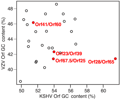
Figure 9: GC content analysis does not show any correlation. The correlation of GC content has decayed during the independent evolution of the two viruses.

3.1 Conservation of the network–aligned Orfs pairs at the sequence level

The pairwise sequence comparison described in Section 2 have not yielded a significant sequence similarity for $2$ node pairs aligned solely due to their interaction similarity.

To further test the possibility of detection of sequence homology homology we have searched for multiple sequence alignments of the protein families to which these Orfs belong. We have extracted the respective families from the VOCs database [3], and compared them using DIALIGN [14], Parallel PRRN [15], MUSCLE [16], T-COFFEE [17], PSALIGN [18], SAM-T99 [19], and MSA [20].

For each pair KSHV 67.5/VZV 25, 28/65, 23/39, 41/60 we have selected from the VOCs database a representative subset of the herpesviral proteins in the same family (at least ten or all proteins) and compared these families using the multiple alignment searching tools. While for the pair 67.5/25 we have found very weak alignment of the corresponding families, for the other three pairs we have detected no sequence similarity. This observation further shows the extend of the evolutionary divergence for the pairs of Orfs.

Returning back to the pairwise alignment we have generated the dot plots for the pairs listed in the Table 1. Here we observe a very clear pattern: while for the Orfs pairs with a high similarity the dot plot is dominated by a single diagonal, with increasing divergence this diagonal disappears among short diagonal lines that correspond to random alignments, see Figure 10. The network–aligned pairs show the dot–plot pattern of an intermediate quality.

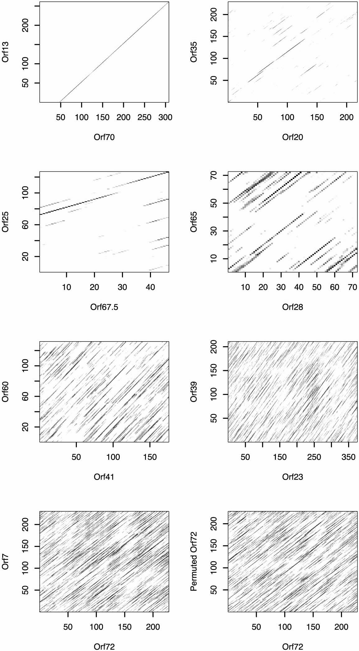
Figure 10: Network alignment allows detection of homologs with poor sequence similarity. With decreasing level of sequence conservation the dominant diagonal in the dot plot disappears among traces of random alignments. From top–left to bottom–right: Orfs KSHV 70/VZV 13, an almost perfect match; Orfs 35/20, a typical match of sequence homologs, Orfs 67.5/25, the pair aligned due to sequence and network conservation; Orfs 28/65, 41/60 and 23/39, the pairs aligned dominantly or only because of interaction conservation; Orfs 72/7, spurious sequence homologs not aligned by the network alignment; Orf 72/permuted Orf 72, comparison with a random sequence. The sliding window of size 30 has been used for the generation of the dot plots.

a) sequenceAlign

Query=  KSHV-BC1-Orf67.5            Length= 80
Sbjct=  VZV-Oka_p-Orf25             Length= 156
Score=  0.2433
logMu  -6.798, logNu 0.006, logAlpha 0.049,
Matrix: blosum50

Q:                EYAS--------------------------------------------------------
S:                YESENASEHHPELEDVFSENTGDSNPSMGSSDSTRSISGMRARDLITDTDVNLLNIDALE
                    +

Q:                ----------------DQLLPRDMQILFPTIYCRLNAINYCQYLKTFLVQR--------A
S:                SKYFPADSTFTLSVWFENLIPPEIEAILPTTDAQLNYISFTSRLASVLKHKESNDSEKSA
                                  ++L+P +++ ++PT   +LN I++ + L + L ++        A

Q:                QPAACDHTLVLESKVDTVRQVLRKIVSTDAVFSEA
S:                YVVPCEHSASVTRRRERFAGVMAKFLDLHEILKDA
                      C+H+  +  + +    V+ K +    ++ +A

b) clustalW

Sequence 1: KSHV-BC1-Orf67.5               80 aa
Sequence 2: VZV-Oka_p-Orf25                156 aa
Alignment Score 57
CLUSTAL W (1.81) multiple sequence alignment

KSHV-BC1-Orf67.5  --------MEYAS----DQLLPRDMQILFPTIYCRLNAINYCQYLKTFLVQRAQP-----
VZV-Oka_p-Orf25   ESKYFPADSTFTLSVWFENLIPPEIEAILPTTDAQLNYISFTSRLASVLKHKESNDSEKS
                            ++     ++L+P +++ ++PT  ++LN I++ + L ++L ++ +

KSHV-BC1-Orf67.5  ---AACDHTLVLESKVDTVRQVLRKIVSTDAVFSEARARP
VZV-Oka_p-Orf25   AYVVPCEHSASVTRRRERFAGVMAKFLDLHEILKDA----
                     ++C+H+  +  + + +  V+ K+++ + ++++A

Figure 11: Weak sequence similarity of the KSHV Orf 67.5 and the VZV Orf 25. Both sequenceAlign (a) and clustalW (b) find alignments with 20% (18%) identity over approximately 80 aa. The score of the sequenceAlign alignment is $0.2$, meaning that the random model is almost as likely as the model of evolutionary related sequences. This is also shown by the very high p-value of the clustalW alignment, $p=0.44$. Such a level of sequence similarity cannot prove homology of the two Orfs, if it is not supported by another method.

Sequence 1: KSHV-BC1-028      102 aa
Sequence 2: VZV-Oka_p-065     102 aa
Alignment Score -31
CLUSTAL W (1.81) multiple sequence alignment

KSHV-BC1-028         MSMTSPSPVTGGMVDGSVLVRMATKPPVIGLITVLFLLVIGACVYCCIRVFLAARLWRAT
VZV-Oka_p-065        MAGQNTMEGEAVALLMEAVVTPRAQPNNTTITAIQPSRSAEKCYYSDSENETADEFLRRI
                     M+  ++    +  +  +++V   ++P    + ++        C Y+  +   A ++ R

KSHV-BC1-028         PLGRATVAYQVLRTLGPQAGSHAPPTVGIATQEPYRTIYMPD
VZV-Oka_p-065        GKYQHKIYHRKKFCYITLIIVFVFAMTGAAFALGYITSQFVG
                        + ++ ++      +    ++ + +G A    Y T  + +

Figure 12: Homology of the Orfs KSHV Orf28 and VZV Orf65 cannot be inferred from the sequence comparison only. The alignment produced by sequenceAlign and clustalW are identical. The p-value of the alignment is $p=0.66$, though. Another method is needed to support the homology.

Sequence 1: KSHV-BC1-023         404 aa
Sequence 2: VZV-Oka_p-039        240 aa
Alignment Score 41
CLUSTAL W (1.81) multiple sequence alignment

KSHV-BC1-023         MLRVPDVKASLVEGAARLSTGERVFHVLTSPAVAAMVGVSNPEVPMPLLFEKFGTPDSST
VZV-Oka_p-039        ----------------------------------------------------------MN
                                                                                +

KSHV-BC1-023         LPLYAARHPELSLLRIMLSPHPYALRSHLCVGEETASLGVYLHSKPVVRGHEFEDTQILP
VZV-Oka_p-039        PPQARVSEQTKDLLSVMVNQHP--------------------------------------
                      P   + +   +LL +M++ HP

KSHV-BC1-023         ECRLAITSDQSYTNFKIIDLPAGCRRVPIHAANKRVVIDEAANRIKVFDPESPLPRHPIT
VZV-Oka_p-039        --------------------------------------EEDAKVCKSSDNSPLYNTMVML
                                                           +E A+  K  D ++      +

KSHV-BC1-023         PRAGQTRSILKHNIAQVCERDIVSLNTDNEAASMFYMIGLRRPRLGESPVCDFNTVTIME
VZV-Oka_p-039        SYGGDTDLLLSS----ACTRTSTVNRSAFTQHSVFYIIST----VLIQPICCIFFFFYYK
                     + +G+T  +L+     +C R  +  ++     S+FY+I+     +  +P+C +  +   +

KSHV-BC1-023         RANNSITFLPKLKLNRLQHLFLKHVLLRSMGLENIVSCFSSLYGAELAPAKTHEREFFGA
VZV-Oka_p-039        ATRCMLLFTAGLLLTILHHFRLIIMLL----------CVYRNIRSDLLPLSTSQQLLLGI
                      ++  + F + L L+ L+H+ L  +LL          C+     ++L P +T ++ ++G

KSHV-BC1-023         LLERLKRRVEDAVFCLNTIEDFPFREPIRQPPDCSKVLIEAMEKYFMMCSPKDRQSAAWL
VZV-Oka_p-039        IVVTRT-----MLFCITAYYTLFIDTRVFFLITGHLQSEVIFPDSVSKILPVSWGPSPAV
                     ++   +      +FC+++   + +   +             + + +    P +  +++ +

KSHV-BC1-023         GAGVVELICDGNPLSEVLGFLAKYMPIQKECTGNLLKIYALLTV
VZV-Oka_p-039        LLVMAAVIYAMDCLVDTVSFIG-----PRVWVRVMLKTSISF--
                        ++ +I   + L ++++F++      +  +  +LK    +

Figure 13: Homology of KSHV Orf 23 and VZV Orf 39 cannot be inferred from sequence similarity. The sequenceAlign does not find any nontrivial alignment and the clustalW alignment has the p-value equal to $0.43$. Another method is needed to support the homology.

Sequence 1: KSHV-BC1-041         205 aa
Sequence 2: VZV-Oka_p-060        160 aa
Alignment Score -42
CLUSTAL W (1.81) multiple sequence alignment

KSHV-BC1-041         MAGFTLKGGTSGDLVFSSHANLLFSTSMGYFLHAGSPRSTAGTGGEPNPRHITGPDTEGN
VZV-Oka_p-060        ---------MASHKWLLQMIVFLKTITIAYCLHLQDDTPLFFGAKPLSDVSLIITEPCVS
                               +++  + +   +L + +++Y LH  +  +    +   +   +  +++  +

KSHV-BC1-041         GEHRNSPNLCGFVTWLQSLTTCIERALNMPPDTSWLQLIEEVIPLYFHRRRQTSFWLIPL
VZV-Oka_p-060        SVYEAWDYAAPPVSNLSEALSGIVVKTKCP--------VPEVILWFKDK--QMAYWTNPY
                     + ++     +  V+ L++  + I    + P        + EVI  + ++  Q ++W  P

KSHV-BC1-041         SHCEGIPVCPPLPFDCLAPRLFIVTKSGPMCYRAGFSLPVDVNYLFYLEQTLKAVRQVSP
VZV-Oka_p-060        VTLKGLTQSVGEEHKSGDIRDALLDALSGVWVDS------------------------TP
                        +G++ +    +++   R  ++   + +   +                        +P

KSHV-BC1-041         QEHNPQDAKEMTLQLEAWTRLLSLF
VZV-Oka_p-060        SSTNIPENGCVWGADRLFQRVCQ--
                     ++ N  +   +    + + R+ +

Figure 14: ClustalW alignment of the KSHV Orf 41 and VZV Orf 60 is not statistically significant. Its p-value is 0.94. SequenceAlign does not find any nontrivial alignment.

3.2 Conserved links typically connect alike Orfs

To examine the relationship between function of the proteins and the conservation of links among them, we analyse the likeliness of the conservation of the links among the proteins with similar functions and of the conservation of the links between the proteins with dissimilar functions.

First we test if the conserved links are more likely to connect alike proteins. To do so, we group the Orfs to two functional classes: the protein belongs either to the class of ‘structure–related’ proteins (classes: capsid/core protein, membrane/glycoprotein, virion protein, virion assembly) or to the class of ‘information–processing’ proteins (DNA replication, gene expression regulation, nucleotide repair/metabolism, host–virus interaction). We calculate the frequencies $p(f_{i},f_{j})$ of functional annotations $f_{i}$, $f_{j}$ of adjacent Orfs $i$ and $j$ in the subgraph containing all sequence homologs (resp. all network–aligned Orfs),

$$p(g,h)=\frac{\sum_{links}\delta(f_{i}=g)\delta(f_{j}=h)}{\sum_{links}1}.$$ (40)

We evaluate this sum separately for all the links in the subgraph ($p_{A}$), the conserved links only ($p_{M}$) and for the nonconserved (mismatching) links in the subgraph ($p_{MM}$).

Then we calculate the mutual information as the measure of the influence of the functional annotation of the adjacent Orfs on the link state,

$$I=\sum_{g}\sum_{h}p(g,h)\ln\frac{p(g,h)}{p(g)p(h)},$$ (41)

where $p(g)$ is the marginal $p(g)=\sum_{h}p(g,h)$. Keeping the subscripts we find: $I_{A}=0.0014$ for the subgraph of sequence homologs ($0.0092$ for the alignment subgraph), $I_{M}=0.0743$ ($0.1178$), and $I_{MM}=1\times 10^{-6}$ ($0.0001$). Clearly, the largest mutual information of functional annotation of adjacent Orfs is among nodes connected by matching links (by a factor of 100 or more). We have evaluated also the frequency tables for the complete protein interaction networks, $p_{K}$ and $p_{V}$. Not surprisingly, the mutual information is small for these graphs $I_{K}=0.0030$, and $I_{V}=0.0052$.

To estimate the p-value of such a mutual information we have reshuffled the positions of the conserved links randomly and we have evaluated the mutual information $I_{M}$ for such randomised graphs. The probability of finding equal or better mutual information $I_{M}$ in an ensemble of $10^{5}$ graphs generated in this way has been taken as the p-value. The estimates are $0.12$ for the subgraph of sequence homologs and $0.05$ for the alignment subgraph.

Secondly, we test if the links between similar proteins are more likely to be conserved. Taking the subgraph of the sequence homologs as the basis of our analysis, we create the matrix $n_{F}(a,b)$ defined in the following way: $n_{F}(0,0)$ is the number of pairs of the alike Orfs between which there is a link in neither species; $n_{F}(1,0)$ is the number of the pairs of the alike Orfs that are connected by a link in KSHV solely; $n_{F}(0,1)$ the same for VZV; and $n_{F}(1,1)$ is the number of conserved links between alike Orfs. We create the second matrix $n_{D}$ defined similarly for the pairs of Orfs with unlike functional annotation.

Then we define the conservation ratio $p_{F}$ as the ratio of the number of conserved links and the total number of links

$$c_{F}=n_{F}(1,1)/(n_{F}(0,1)+n_{F}(1,0)+n_{F}(1,1)).$$ (42)

In the same way we define $c_{D}$ for the links between unlike Orfs.

A rough estimate of the odds in the link conservation can be expressed as the ratio of the two conservation ratios

$$C_{F}=c_{F}/c_{D}.$$ (43)

Its value is $1.62$, that is the links between alike Orfs are $62\%$ more likely to be conserved than the links between unlike Orfs ($c_{F}=0.15$, $c_{D}=0.09$). The p-value evaluated over the same graph with a randomised annotation list is $0.47$.

More refined estimate of the odds which takes in consideration also the link statistics of the two networks uses mutual information, $I_{F}$ and $I_{D}$. The mutual information expresses the level of correlation of the presence of the link in the two networks. If we normalise the frequencies $n_{F}$, $p_{F}(a,b)=n_{F}(a,b)/\sum_{c,d}n_{F}(c,d)$, we may write the mutual information as

$$I_{F}=\sum_{a,b}p_{F}(a,b)\ln\frac{p_{F}(a,b)}{p_{F}^{A}(a)p_{F}^{B}(b)},$$ (44)

where the marginals are defined as $p_{F}^{A}(a)=\sum_{b}p_{F}(a,b)$ and $p_{F}^{B}(a)=\sum_{a}p_{F}(a,b)$. In the same way we define the mutual information $I_{D}$ for the unlike Orfs pairs. For the subgraph of the sequence homologs the mutual information reads $I_{F}=0.049$, $I_{D}=0.005$. Defining the final information odds, $D_{F}=I_{F}/I_{D}$, we get $D_{F}=9.58$ with the p-value 0.13 (the same test as for $C_{F}$).

References

- [1] Havgaard JH, Lyngso RB, Stormo GD, Gorodkin J (2005) Bioinformatics 21(9): 1815–24.
- [2] Ponomarenko JV, Bourne PE, Shindyalov IN (2005) Proteins: Structure, Function and Bioinformatics 58: 855–865.
- [3] Zhang Y and Skolnick J (2005) Nucleic Acids Res. 33(7): 2302–2309.
- [4] Uetz P, Dong Y-A, Zeretzke C, Atzler C, Baiker A, Berger B, Rajagopala SV, Roupelieva M, Rose D, Fossum E, Haas J (2006) Science 311: 239–242.
- [5] McGeoch DJ and Cook S (1994) J. Mol. Biol. 238: 9–22.
- [6] Mar Albà M, Das R, Orengo CA, and Kellam P (2001) Genome Res. 11: 43–54.
- [7] King MC and Wilson AC (1975) Science 188: 107–166.
- [8] Beltrao P, Serrano L (2007) PLoS Comput Biol. 3(2): e25.
- [9] Berg J and Lässig M (2006) Proc. Natl. Acad. Sci. USA 103(29): 10967–10972.
- [10] Koonin EV, Mushegian AR, Bork P (1996) Trends Genet. 12(9): 334–336.
- [11] Sharan R, Suthram S, Kelley RM, Kuhn T, McCuine S, Uetz P, Sittler T, Karp RM, and Ideker T (2005) Proc Natl Acad Sci USA 102(6): 1974–1979.
- [12] S. Bandyopadhyay, R. Sharan, and T. Ideker (2006) Genome Res. 16: 428–435.
- [13] Trusina A, Sneppen K, Dodd IB, Shearwin KE, Egan JB (2005) PLoS Computational Biology 1(7): e74.
- [14] Hiscock D, Upton C (2000) Bioinformatics 16: 484–485.
- [15] Bao Y, Federhen S, Leipe D, Pham V, Resenchuk S, Rozanov M, Tatusov R, and Tatusova T (2004) J Virol. 78(14): 7291–7298.
- [16] Davison AJ, Scott JE (1986) J Gen Virol. 67(9): 1759–1816.
- [17] Russo JJ, Bohenzky RA, Chien MC, Chen J, Yan M, Maddalena D, Parry JP, Peruzzi D, Edelman IS, Chang Y, Moore PS (1996) Proc Natl Acad Sci USA 93(25): 14862–14867.
- [18] Kirkpatrick, S., C. D. Gelatt Jr., M. P. Vecchi, (1983) Science 220: 671–680.
- [19] Hwa T and Lässig M (1996) Phys. Rev. Lett. 76: 2591–2594.
- [20] Mar Albà M, Lee D, Pearl FMG, Shepherd AJ, Martin N, Orengo CA, and Kellam P (2001) Nuleic Acids Research 29(1): 133–136.
- [21] Reynolds AE, Fan Y, Baines JD (2000) Virology 266(2): 310–318.
- [22] Cohen JI, Sato H, Srinivas S, and Lekstrom K (2001) Virology 280: 62–71.
- [23] Jenner RG, Mar Albà M, Boshoff C, and Kellam P (2001) Journal of Virology 75(2): 891–902.
- [24] Paulose-Murphy M, Ha N-K, Xiang C, Chen Y, Gillim L, Yarchoan R, Meltzer P, Bittner M, Trent J, and Zeichner S (2001) Journal of Virology 75(10): 4843–4853.
- [25] Lu M, Suen J, Frias C, Pfeiffer R, Tsai M-H, Chuang E, and Zeichner SL (2004) Journal of Virology 78(24): 13637–13652.
- [26] Zhu FX, Chong JM, Wu L, and Yuan Y (2005) Journal of Virology 79(2): 800–811.
- [27] Thompson JD, Higgins DG and Gibson TJ (1994) Nucleic Acids Research 22: 4673–4680.
- [28] Wu FY, Ahn J-H, Alcendor DJ, Jang W-J, Xiao J, Hayward DS and Hayward GS (2001) Journal of Virology 75(3): 1487–1506.
- [29] Marešová L, Kutinová L , Ludvíková V, Žák R, Mareš M, and Němečková Š (2000) Journal of General Virology 81: 1545–1552.
- [30] Kelley BP, Sharan R, Karp RM, Sittler T, Root DE, Stockwell BR, Ideker T (2003) Proc Natl Acad Sci USA 100(20): 11394–11399.
- [31] Oliver S (2000) Nature 403: 601–603.

References

- [1] Uetz P, Dong Y-A, Zeretzke C, Atzler C, Baiker A, Berger B, Rajagopala SV, Roupelieva M, Rose D, Fossum E, Haas J (2006) Herpesviral protein networks and their interaction with the human proteome. Science 311: 239–242.
- [2] Mar Albà M, Lee D, Pearl FMG, Shepherd AJ, Martin N, Orengo CA, and Kellam P (2001) VIDA: a virus database system for the organisation of virus genome open reading frames. Nuleic Acids Research 29(1): 133–136.
- [3] Hiscock D, Upton C (2000) Viral Genome Database: A tool for storing and analyzing genes and proteins from complete viral genomes. Bioinformatics 16: 484–485.
- [4] Martello S and Toth P (1987) Linear assignment problems. Annals of Discrete Math. 31: 259–282.
- [5] Kirkpatrick S and Gelatt CD and Vecchi MP (1983) Optimization by Simulated Annealing. Science Vol 220 No 4598: 671–680.
- [6] Meier JP, Kolář M, Mustonen V, Lässig M, and Berg J (2007) R: GraphAlignment Package Manual http://XXX.XXX.XXX/GraphAlignment
- [7] Viterbi AJ (1967) Error bounds for conventional codes and an asymptotically optimum decoding algorithm. IEEE Transactions on Information Theory 13(2): 260–269.
- [8] Bao Y, Federhen S, Leipe D, Pham V, Resenchuk S, Rozanov M, Tatusov R, and Tatusova T (2004) National Center for Biotechnology Information Viral Genomes Project. J Virol. 78(14): 7291–7298.
- [9] Needleman SB, Wunsch CD (1970) A general method applicable to the search for similarities in the amino acid sequence of two proteins J. Mol. Biol., 48, 443-453.
- [10] Henikoff S and Henikoff JG (1992) Amino acid substitution matrices from protein blocks Proc. Natl. Acad. Sci. USA, 89, 10915-10919.
- [11] Yu Y-K and Hwa T, (2001) Statistical significance of probabilistic sequence alignment and related local Hidden Markov Models Journal of Computational Biology, Vol. 8, Num. 3, 249-282.
- [12] Thompson JD, Higgins DG and Gibson TJ (1994) CLUSTAL W: improving the sensitivity of progressive multiple sequence alignment through sequence weighting, positions-specific gap penalties and weight matrix choice. Nucleic Acids Research 22: 4673–4680.
- [13] Vlček Č, Beneš V, Lu Z, Kutish GF, Pačes V, Rock D, Letchworth GJ and Schwyzer M, (1995) Nucleotide sequence analysis of a 30-kb region of the bovine herpesvirus 1 genome which exhibits a colinear gene arrangement with the UL21 to UL4 genes of herpes simplex virus Virology 210 (1): 100–108.
- [14] Morgenstern B (2004) DIALIGN: Multiple DNA and protein sequence alignment at BiBiServ. Nucleic Acids Research 32: W33–W36.
- [15] Gotoh O (1996) Significant improvement in accuracy of multiple protein sequence alignments by iterative refinement as assessed by reference to structural alignments. J. Mol. Biol. 264: 823–838.
- [16] Edgar RC (2004) MUSCLE: multiple sequence alignment with high accuracy and high throughput. Nucleic Acids Research 32(5): 1792–97.
- [17] Notredame C, Higgins D, Heringa J (2000) T-Coffee: A novel method for multiple sequence alignments. Journal of Molecular Biology 302: 205–217.
- [18] Sze S-H, Lu Y, and Yang Q (2006) A polynomial time solvable formulation of multiple sequence alignment. Journal of Computational Biology 13: 309–319.
- [19] Karplus K, Barrett C, and Hughey R (1998) Hidden Markov Models for detecting remote protein homologies. Bioinformatics 14(10): 846–856.
- [20] Lipman D, Altschul S, and Kececioglu J (1989) A Tool for Multiple Sequence Alignment Proc. Natl. Acad. Sci. USA 86: 4412–4415.