Abstract

A system with Bose-Einstein condensate is considered in the frame of the self-consistent mean-field approximation, which is conserving, gapless, and applicable for arbitrary interaction strengths and temperatures. The main attention is paid to the thorough analysis of the condensate and superfluid fractions in the whole range of the interaction strength, between zero and infinity, and for all temperatures between zero and the critical point $T_{c}$. The normal and the anomalous averages are shown to be of the same order for almost all interactions and temperatures, except the close vicinity of $T_{c}$. But even in the vicinity of the critical temperature, the anomalous average cannot be neglected, since only in the presence of the latter the phase transition at $T_{c}$ becomes of second order, as it should be. Increasing temperature influences the condensate and superfluid fractions in a similar way, by diminishing them. But their behavior with respect to the interaction strength is very different. For all temperatures, the superfluid fraction is larger than the condensate fraction. These coincide only at $T_{c}$ or under zero interactions. For asymptotically strong interactions, the condensate is almost completely depleted, even at low temperatures, while the superfluid fraction can be close to one.

PACS number(s): 03.75.Hh, 03.75.Kk, 03.75.Nt, 05.30.Ch

1 Introduction

The relation between Bose-Einstein condensation (BEC) and superfluidity is of long-standing interest. The most thorough studies, both experimental and theoretical, of Bose-system properties have been accomplished for the region of low temperatures and weak interactions (see review works [1–7]), where the Bogolubov approximation [8,9] is applicable. In this region, almost the entire system is Bose-condensed, being just slightly depleted by interactions, at the same time, practically the whole system is superfluid. When the condensate and superfluid fractions are so close to each other, one often uses as synonyms the terms ”Bose-condensed” and ”superfluid”.

The opposite situation occurs for strongly interacting liquids, such as superfluid ⁴He, where the superfluid fraction at low temperatures almost reaches one, while the condensate fraction never exceeds the values of the order of $10\%$. The superfluid properties of helium are among the best-measured in experimental physics, as can be inferred, e.g., from the books [10–13]. The BEC fraction in superfluid helium, has been measured by using the $x$-ray scattering [14] and deep-inelastic neutron scattering [15]. Theoretical investigation, because of strong interactions between helium atoms, is rather complicated and mainly is done numerically, for instance, by means of Monte Carlo techniques [16,17].

It would be important to understand the behavior of the condensate and superfluid fractions of the same system in the whole region of varying interaction strength and temperature. Present-day Feshbach-resonance techniques do allow for the variation of the interaction strength in a very wide range [18,19]. It is the aim of the present paper to investigate the condensate and superfluid fractions for all temperatures between zero and the critical temperature $T_{c}$ and for all interaction strengths between zero and infinity. Such an analysis can be accomplished in the frame of the self-consistent mean-field theory [20–25], which is conserving, gapless, satisfies all thermodynamic relations and conservation laws. It was shown that this theory yields good agreement with Monte Carlo simulations for weak as well as strong interactions [24] and can also be applied for Bose systems in random potentials with arbitrary strong strength of disorder [25].

Studying here the condensate and superfluid fractions, we analyse their properties both analytically and numerically. We use the system of units with $\hbar\equiv 1$ and $k_{B}\equiv 1$.

2 Uniform Equilibrium System

Let us consider a uniform equilibrium Bose system with BEC. The appearance of BEC, as is known [26–28], is equivalent to the gauge symmetry breaking. The most convenient way to realize the latter is by means of the Bogolubov operator shift [29,30] representing the Bose field operator as the sum

$$\hat{\psi}({\bf r})\equiv\eta({\bf r})+\psi_{1}({\bf r})\;.$$ (1)

The first term here is the condensate wave function normalized to the number of condensed atoms

$$N_{0}=\int|\eta({\bf r})|^{2}\;d{\bf r}\;,$$ (2)

and the second term is the field operator of uncondensed atoms, satisfying the Bose commutation relations and the normalization to the number of uncondensed atoms

$$N_{1}=\int<\psi_{1}^{\dagger}({\bf r})\psi_{1}({\bf r})>d{\bf r}\;.$$ (3)

The angle brackets mean, as usual, statistical averaging. The condensate function $\eta({\bf r})$ and the operator of uncondensed atoms $\psi_{1}({\bf r})$ are treated as independent variables, orthogonal to each other,

$$\int\eta^{*}({\bf r})\psi_{1}({\bf r})\;d{\bf r}=0\;.$$ (4)

The total average density is the sum

$$\rho=\rho_{0}+\rho_{1}$$ (5)

of the condensate density $\rho_{0}$ and the density $\rho_{1}$ of uncondensed atoms,

$$\rho_{0}\equiv\frac{N_{0}}{V}\;,\qquad\rho_{1}\equiv\frac{N_{1}}{V}\;,$$ (6)

where $V$ is the system volume. The atoms are assumed to interact with each other through the local interaction potential

$$\Phi({\bf r})=\Phi_{0}\delta({\bf r})\;,\qquad\Phi_{0}\equiv 4\pi\;\frac{a_{s}}{m}\;,$$ (7)

with $a_{s}$ being the scattering length and $m$ being atomic mass.

For a uniform equilibrium system, the condensate function is constant,

$$\eta({\bf r})=\sqrt{\rho_{0}}\;.$$ (8)

The field operator of uncondensed atoms can be expanded over plane waves

$$\varphi_{k}({\bf r})\equiv\frac{e^{i{\bf k}\cdot{\bf r}}}{\sqrt{V}}\;,$$

which gives

$$\psi_{1}({\bf r})=\sum_{k}a_{k}\varphi_{k}({\bf r})\;.$$ (9)

From the orthogonality equation (4) it follows that

$$\lim_{k\rightarrow 0}a_{k}=0\;.$$ (10)

Therefore, in expansion (9), the summation is over ${\bf k}\neq 0$. This condition can either be shown explicitly in Eq. (9) or just one can keep in mind property (10).

Accomplishing the Bogolubov shift for the field operator (1), we have the grand Hamiltonian

$$H=\sum_{n=0}^{4}H^{(n)}$$ (11)

consisting of five terms, labelled according to their order with respect to $a_{k}$ and $a_{k}^{\dagger}$. The zero-order term does not contain the field operators of uncondensed atoms

$$H^{(0)}=\left(\frac{1}{2}\;\rho_{0}\Phi_{0}-\mu_{0}\right)N_{0}\;.$$ (12)

The first-order term is identically zero,

$$H^{(1)}=0\;,$$ (13)

because of the orthogonality equation (4). The second-order term is

$$H^{(2)}=\sum_{k}\left[\left(\frac{k^{2}}{2m}+2\rho_{0}\Phi_{0}-\mu_{1}\right)a_{k}^{\dagger}a_{k}+\frac{1}{2}\;\rho_{0}\Phi_{0}\left(a_{k}^{\dagger}a_{-k}^{\dagger}+a_{-k}a_{k}\right)\right]\;.$$ (14)

Respectively, one has the third-order term

$$H^{(3)}=\sqrt{\frac{\rho_{0}}{V}}\;\Phi_{0}\;\sum_{p,q}\left(a_{q}^{\dagger}a_{q-p}a_{p}+a_{p}^{\dagger}a_{q-p}^{\dagger}a_{q}\right)$$ (15)

and the fourth-order term

$$H^{(4)}=\frac{\Phi_{0}}{2V}\;\sum_{k,p,q}a_{p}^{\dagger}a_{q}^{\dagger}a_{k+p}a_{q-k}\;.$$ (16)

In Eqs. (14), (15), and (16), the sums do not contain the terms with the operators $a_{k}$, for which ${\bf k}=0$, due to the limiting condition (10).

The momentum distribution of uncondensed atoms is given by the normal average

$$n_{k}\;\equiv\;<a_{k}^{\dagger}a_{k}>\;.$$ (17)

Because of the broken gauge symmetry, there also appears the anomalous average

$$\sigma_{k}\;\equiv\;<a_{k}a_{-k}>\;.$$ (18)

The normal and anomalous averages are equally important and neither of them can be neglected. Omitting the anomalous average would make the theory not self-consistent and would yield a spurious system instability [5,31]. Summing Eqs. (17) and (18) gives the density of uncondensed atoms

$$\rho_{1}=\frac{1}{V}\;\sum_{k}n_{k}$$ (19)

and the anomalous average

$$\sigma_{1}=\frac{1}{V}\;\sum_{k}\sigma_{k}\;,$$ (20)

for which the value $|\sigma_{1}|$ defines the density of pair-correlated atoms [32].

Applying for terms (15) and (16) the Hartree-Fock-Bogolubov approximation and involving the Bogolubov canonical transformation

$$a_{k}=u_{k}b_{k}+u_{-k}^{*}b_{-k}^{\dagger}\;,$$

we reduce [24] the grand Hamiltonian (11) to the form

$$H=E_{B}+\sum_{k}\varepsilon_{k}b_{k}^{\dagger}b_{k}\;,$$ (21)

in which

$$E_{B}=-\left(\frac{1}{2}\;\rho_{0}+2\rho_{1}+\sigma_{1}\right)\Phi_{0}N_{0}\;-\;\frac{\Phi_{0}}{2\rho}\left(2\rho_{1}^{2}+\sigma_{1}^{2}\right)N+\frac{1}{2}\;\sum_{k}(\varepsilon_{k}-\omega_{k})$$ (22)

is a nonoperator quantity;

$$\varepsilon_{k}=\sqrt{(ck)^{2}+\left(\frac{k^{2}}{2m}\right)^{2}}$$ (23)

is the Bogolubov-type spectrum, but with the sound velocity $c$ defined by the equation

$$mc^{2}=(\rho_{0}+\sigma_{1})\Phi_{0}\;.$$ (24)

For the momentum distribution (17), we get

$$n_{k}=\frac{\omega_{k}}{2\varepsilon_{k}}\;{\rm coth}\left(\frac{\varepsilon_{k}}{2T}\right)\;-\;\frac{1}{2}\;,$$ (25)

where $T$ is temperature and

$$\omega_{k}\equiv\frac{k^{2}}{2m}+mc^{2}\;.$$ (26)

And for the anomalous average (18), we find

$$\sigma_{k}=-\;\frac{mc^{2}}{2\varepsilon_{k}}\;{\rm coth}\left(\frac{\varepsilon_{k}}{2T}\right)\;.$$ (27)

We may notice that

$$n_{k}+\frac{\omega_{k}}{mc^{2}}\;\sigma_{k}+\frac{1}{2}=0\;,$$

which indicates that $\sigma_{k}$ is, generally, of the same order as $n_{k}$.

Using Eq. (25) and passing in the standard way from summation over momenta to their integration, we obtain for the density of uncondensed atoms (19)

$$\rho_{1}=\frac{(mc)^{3}}{3\pi^{2}}\left\{1+\frac{3}{2\sqrt{2}}\;\int_{0}^{\infty}\;\left(\sqrt{1+x^{2}}-1\right)^{1/2}\left[{\rm coth}\left(\frac{mc^{2}}{2T}\;x\right)-1\right]\;dx\right\}\;.$$ (28)

For the anomalous average (20), using Eq. (27), we find

$$\sigma_{1}=\sigma_{0}\;-\;\frac{(mc)^{3}}{2\sqrt{2}\;\pi^{2}}\;\int_{0}^{\infty}\;\frac{\left(\sqrt{1+x^{2}}-1\right)^{1/2}}{\sqrt{1+x^{2}}}\left[{\rm coth}\left(\frac{mc^{2}}{2T}\;x\right)-1\right]\;dx\;,$$ (29)

where in the calculation of the term

$$\sigma_{0}=\frac{(mc)^{2}}{\pi^{2}}\;\sqrt{m\rho_{0}\Phi_{0}}$$ (30)

the dimensional regularization [24] is employed, in line with the general rules of the dimensional regularization [5,33].

3 Condensate and Superfluid Fractions

Our main aim here is to study the condensate and superfluid fractions. The condensate fraction

$$n_{0}\equiv\frac{N_{0}}{N}=1-n_{1}$$ (31)

can be found by calculating the normal fraction

$$n_{1}\equiv\frac{N_{1}}{N}=\frac{\rho_{1}}{\rho}\;,$$ (32)

with the normal density (28).

The superfluid fraction can be represented [2,25] as

$$n_{s}=1-\frac{2Q}{3T}\;,$$ (33)

where $Q$ is the dissipated heat,

$$Q\equiv\frac{\Delta^{2}(\hat{\bf P})}{2mN}\;,$$ (34)

expressed through the dispersion

$$\Delta^{2}(\hat{\bf P})\;\equiv\;<\hat{\bf P}^{2}>-<\hat{\bf P}>^{2}$$

of the total momentum operator $\hat{\bf P}$. For the dissipated heat, in the considered mean-field approximation, we have

$$Q=\frac{1}{\rho}\;\int\frac{k^{2}}{2m}\left(n_{k}+n_{k}^{2}-\sigma_{k}^{2}\right)\frac{d{\bf k}}{(2\pi)^{3}}\;.$$ (35)

Substituting here Eqs. (25) and (27), we get

$$Q=\frac{1}{8m\rho}\;\int\;\frac{k^{2}}{{\rm sinh}^{2}(\varepsilon_{k}/2T)}\;\frac{d{\bf k}}{(2\pi)^{3}}\;.$$ (36)

The latter equation can be transformed to

$$Q=\frac{(mc)^{5}}{\sqrt{2}(2\pi)^{3}m\rho}\;\int_{0}^{\infty}\;\frac{(\sqrt{1+x^{2}}-1)^{3/2}\;x\;dx}{\sqrt{1+x^{2}}\;{\rm sinh}^{2}(mc^{2}x/2T)}\;.$$ (37)

For the following analysis, it is convenient to introduce dimensionless quantities. We define the gas parameter

$$\gamma\equiv\rho^{1/3}a_{s}\;,$$ (38)

measuring the interaction strength, and the dimensionless temperature

$$t\equiv\frac{mT}{\rho^{2/3}}\;.$$ (39)

We introduce the dimensionless sound velocity

$$s\equiv\frac{mc}{\rho^{1/3}}$$ (40)

and the dimensionless anomalous average

$$\sigma\equiv\frac{\sigma_{1}}{\rho}\;.$$ (41)

In terms of these notations, the dimensionless velocity (40), in view of Eq. (24), satisfies the equation

$$s^{2}=4\pi\gamma(n_{0}+\sigma)\;.$$ (42)

The condensate fraction (31) is expressed through the normal fraction (32), for which we have

$$n_{1}=\frac{s^{3}}{3\pi^{2}}\left\{1+\frac{3}{2\sqrt{2}}\;\int_{0}^{\infty}\;\left(\sqrt{1+x^{2}}-1\right)^{1/2}\left[{\rm coth}\left(\frac{s^{2}x}{2t}\right)-1\right]\;dx\right\}\;.$$ (43)

The anomalous average (41), according to Eqs. (29) and (30), becomes

$$\sigma=\frac{2s^{2}}{\pi^{3/2}}\;\sqrt{\gamma n_{0}}\;-\;\frac{s^{3}}{2\sqrt{2}\;\pi^{2}}\;\int_{0}^{\infty}\;\frac{(\sqrt{1+x^{2}}-1)^{1/2}}{\sqrt{1+x^{2}}}\;\left[{\rm coth}\left(\frac{s^{2}x}{2t}\right)-1\right]\;dx\;.$$ (44)

And the superfluid fraction (33) takes the form

$$n_{s}=1\;-\;\frac{s^{5}}{6\sqrt{2}\;\pi^{2}t}\;\int_{0}^{\infty}\;\frac{(\sqrt{1+x^{2}}-1)^{3/2}x\;dx}{\sqrt{1+x^{2}}\;{\rm sinh}^{2}(s^{2}x/2t)}\;.$$ (45)

Equations (42) to (45), together with the relation $n_{0}=1-n_{1}$, define all characteristics we wish to investigate.

4 Varying Interactions and Temperature

Our aim is to study Eqs. (42) to (45) for the varying interaction strength $\gamma\geq 0$ and temperature $t\geq 0$. First, we find analytic expressions for low temperatures and for the temperature close to the critical point.

A. Low Temperature

At sufficiently low temperature, such that

$$\frac{t}{s^{2}}\ll 1\;,$$ (46)

we find from Eqs. (43) to (45) the asymptotic expansions for the normal fraction

$$n_{1}\simeq\frac{s^{3}}{3\pi^{2}}+\frac{t^{2}}{12s}\;,$$ (47)

the anomalous average

$$\sigma\simeq\frac{2s^{2}}{\pi^{3/2}}\;\sqrt{\gamma n_{0}}\;-\;\frac{t^{2}}{12s}\;,$$ (48)

and for the superfluid fraction

$$n_{s}\simeq 1\;-\;\frac{2\pi^{2}t^{4}}{45s^{5}}\;.$$ (49)

We may notice that between the condensate and superfluid fractions there is the relation

$$(1-n_{s})(1-n_{0})^{5/3}\simeq\frac{2t^{4}}{135\pi(9\pi)^{1/3}}\;.$$ (50)

Substituting these expansions into Eq. (42), we obtain the asymptotic behavior of the dimensionless sound velocity

$$s\simeq s_{0}+at^{2}\qquad(t\rightarrow 0)\;.$$ (51)

Here the zero-temperature term is defined by the equation

$$\pi\left(4\gamma s_{0}^{3}+3\pi s_{0}^{2}-12\pi^{2}\gamma\right)^{2}=192\gamma^{3}s_{0}^{4}\left(3\pi^{2}-s_{0}^{3}\right)\;.$$ (52)

The coefficient $a$ in the second term of Eq. (51) is

$$a=\frac{3\pi^{2}(4\gamma s_{0}^{3}-\pi s_{0}^{2}-12\pi^{2}\gamma)}{16(2\gamma s_{0}^{6}+3\pi s_{0}^{5}-18\pi^{2}\gamma s_{0}^{3}+36\pi^{4}\gamma)}\;.$$ (53)

Using expansion (51) in Eq. (48) gives the anomalous average

$$\sigma\simeq\sigma_{0}+bt^{2}\;,$$ (54)

in which

$$\sigma_{0}=\frac{4\gamma s_{0}^{3}+3\pi s_{0}^{2}-12\pi^{2}\gamma}{12\pi^{2}\gamma}\;,\qquad b=-\;\frac{\sqrt{\pi}}{12\sqrt{\gamma}}\left[1+\frac{2\gamma s_{0}^{3}}{\pi^{5}\sigma_{0}}\left(28s_{0}^{3}+\pi^{2}-48\pi^{2}a\right)\right]\;.$$ (55)

Finally, we obtain the asymptotic temperature expansions for the condensate fraction

$$n_{0}\simeq 1\;-\;\frac{s_{0}^{3}}{3\pi^{2}}\;-\;\frac{\pi^{2}+12as_{0}^{3}}{12\pi^{2}s_{0}}\;t^{2}$$ (56)

and for the superfluid fraction

$$n_{s}\simeq 1\;-\;\frac{2\pi^{2}}{45s_{0}^{5}}\;t^{4}\;.$$ (57)

Equations (56) and (57) show that $n_{s}>n_{0}$.

In order to specify the behavior of $n_{0}$ and $n_{s}$ as functions of the interaction strength, let us consider two limiting cases, of weak and strong interactions. When the interaction is weak, such that $\gamma\rightarrow 0$, Eqs. (52) and (53) give

$$s_{0}\simeq 2\sqrt{\pi}\;\gamma^{1/2}+\frac{16}{3}\;\gamma^{2}\;,\qquad a\simeq-\;\frac{1}{12}\qquad(\gamma\rightarrow 0)\;.$$ (58)

Then the sound velocity (51) is

$$s\simeq 2\sqrt{\pi}\;\gamma^{1/2}\;-\;\frac{t^{2}}{12}\;.$$ (59)

Remembering condition (46), we see that the considered expansions are valid for the low temperatures for which

$$t\ll\gamma\ll 1\;.$$ (60)

For the anomalous average (54), we get

$$\sigma\simeq\frac{8\gamma^{3/2}}{\sqrt{\pi}}\left(1\;-\;\frac{t^{2}}{192\gamma^{2}}\right)\;.$$ (61)

The condensate fraction (56) becomes

$$n_{0}\simeq 1\;-\;\frac{8\gamma^{3/2}}{3\sqrt{\pi}}\left(1+\frac{t^{2}}{64\gamma^{2}}\right)\;,$$ (62)

which is in agreement with the known temperature expansion for the weakly interacting Bose gas [5], first derived by Lee and Yang [34]. And for the superfluid fraction (57), we have

$$n_{s}\simeq 1\;-\;\frac{\gamma^{3/2}}{720\sqrt{\pi}}\left(\frac{t}{\gamma}\right)^{4}\;.$$ (63)

Noting that

$$\frac{n_{s}}{n_{0}}\simeq 1+\frac{8\gamma^{3/2}}{3\sqrt{\pi}}\left(1+\frac{t^{2}}{64\gamma^{2}}\right)\;,$$ (64)

we clearly see that $n_{s}>n_{0}$, though they are close to each other when $\gamma\ll 1$ and $t\ll 1$.

In the opposite case of very strong interactions, when $\gamma\rightarrow\infty$, Eqs. (52) and (53) yield

$$s_{0}\simeq\left(3\pi^{2}\right)^{1/3}-\;\frac{\pi}{64}\left(\frac{\pi}{3}\right)^{2/3}\gamma^{-3}\;,\qquad a\simeq-\;\frac{1}{36}\qquad(\gamma\rightarrow\infty)\;.$$ (65)

The sound velocity (51) behaves as

$$s\simeq\left(3\pi^{2}\right)^{1/3}-\;\frac{t^{2}}{36}\;.$$ (66)

For the anomalous average (54), we find

$$\sigma\simeq\frac{(9\pi)^{1/3}}{4}\left(\frac{1}{\gamma}\;-\;\frac{t^{2}}{9\pi}\right)\;.$$ (67)

In this way, we obtain the condensate fraction

$$n_{0}\simeq\frac{\pi}{64}\;\gamma^{-3}+O(t^{4})$$ (68)

and the superfluid fraction

$$n_{s}\simeq 1\;-\;\frac{2}{135\pi(9\pi)^{1/3}}\left(1+\frac{5\pi}{192\gamma^{3}}\right)t^{4}\;.$$ (69)

The ratio

$$\frac{n_{s}}{n_{0}}\simeq\frac{64}{\pi}\;\gamma^{3}\qquad(\gamma\rightarrow\infty)$$ (70)

shows that $n_{s}$ is much larger than $n_{0}$.

B. Critical Region

The analysis of Eqs. (42) to (45) demonstrates that there is the critical temperature

$$t_{c}=\frac{2\pi}{[\zeta(3/2)]^{2/3}}=3.312498\;,$$ (71)

where $n_{0}$, $n_{s}$, $\sigma$, and $s$ all tend to zero. Temperature (71) is the same as the condensation temperature of the ideal Bose gas, as it should be in the case of a mean-field approximation for atoms with local interactions [5].

Considering the critical region close to $t_{c}$, when

$$\frac{s^{2}}{t_{c}}\ll 1\;,$$ (72)

we find from Eqs. (43), (44), and (45) the normal fraction

$$n_{1}\simeq\left(\frac{t}{t_{c}}\right)^{3/2}+\frac{s^{3}}{3\pi^{2}}\;,$$ (73)

the anomalous average

$$\sigma\simeq\frac{2s^{2}}{\pi^{3/2}}\;\sqrt{\gamma n_{0}}\;-\;\frac{st}{2\pi}\;,$$ (74)

and the superfluid fraction

$$n_{s}\simeq 1-\left(\frac{t}{t_{c}}\right)^{3/2}+\frac{\zeta(1/2)}{\zeta(3/2)}\left(\frac{t}{t_{c}}\right)^{1/2}\frac{s^{2}}{t_{c}}\;.$$ (75)

Calculating the last term in Eq. (75), the dimensional regularization was employed.

When temperature $t$ tends to $t_{c}$, then it is convenient to introduce the relative temperature

$$\tau\equiv 1\;-\;\frac{t}{t_{c}}\;\rightarrow\;+0\;,$$ (76)

which tends to zero. Then, solving Eq. (42) results in

$$s\simeq\sqrt{6\pi\gamma}\;\tau^{1/2}$$ (77)

for any $\gamma>0$. Equations (73) and (74) yield the expansions

$$n_{1}\simeq 1\;-\;\frac{3}{2}\;\tau+2\;\sqrt{\frac{6}{\pi}\;\gamma^{3}}\;\tau^{3/2}\;,$$

$$\sigma\simeq-\;\sqrt{\frac{3\gamma}{2\pi}}\;t_{c}\tau^{1/2}+\frac{12\gamma}{\sqrt{\pi}}\;\tau+\sqrt{\frac{3\gamma}{2\pi}}\;t_{c}\tau^{3/2}\;.$$

Using these, we obtain the condensate fraction

$$n_{0}\simeq\frac{3}{2}\;\tau-2\;\sqrt{\frac{6}{\pi}\;\gamma^{3}}\;\tau^{3/2}$$ (78)

and the superfluid fraction

$$n_{s}\simeq\frac{3}{2}\left[1+4\pi\frac{\zeta(1/2)\gamma}{\zeta(3/2)t_{c}}\right]\tau\;.$$ (79)

As we see, because of the ratio

$$\frac{n_{s}}{n_{0}}\simeq 1+4\pi\frac{\zeta(1/2)\gamma}{\zeta(3/2)t_{c}}\;,$$ (80)

the superfluid fraction is again larger than the condensate fraction for all $\gamma>0$.

Strictly speaking, the above expansions for the critical region are valid for not too large gas parameter $\gamma$. This is because the first term in Eq. (29) has been obtained using the dimensional regularization, which results in Eq. (30). The dimensional regularization is known [5] to be asymptotically exact in the limit of weak interactions. The analytical continuation of Eq. (30) to finite interactions may become not accurate for large values of the latter. In the above expansions, we constantly meet the combination $\gamma t$, which is to be smaller than one to make the expansions quantitatively correct. From the inequality $\gamma t\leq 1$, in the critical region, when $t\approx t_{c}$, we get $\gamma\leq 0.3$. Considering in what follows the critical properties of the system, for $\gamma>0.4$, we keep in mind that the behaviour of thermodynamic characteristics for these values of $\gamma$ is only approximate.

The asymptotic behavior of $n_{0}$ and $n_{s}$ in expansions (78) and (79) makes it apparent that both $n_{0}$ and $n_{s}$ tend simultaneously to zero at $t_{c}$, so that BEC coincides with the superfluid transition. This phase transition is of second order, which agrees with the universality theory. According to the latter, the considered Bose system with BEC belongs to the universality class of the 3-dimensional $O(2)$-symmetric spin model, hence, must display the second-order phase transition [5,35,36]. It is worth noting the importance of the anomalous average $\sigma$. Though it tends to zero, as $t\rightarrow t_{c}$, but it cannot be neglected, since $n_{0}$ also tends to zero. Neglecting the anomalous average $\sigma$ would result in the first-order phase transition [5], which is not correct. In addition, omitting $\sigma$ would make the system unstable at all temperatures [31].

C. Numerical Solution

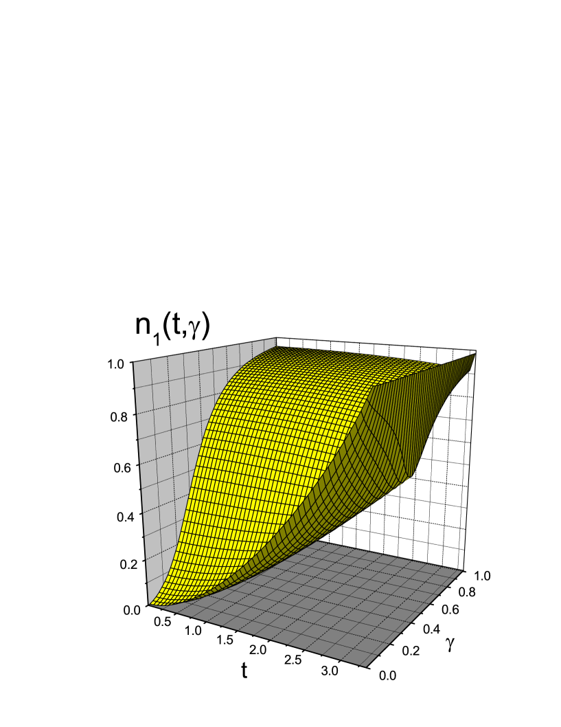
Figure 1: Fraction of uncondensed atoms $n_{1}=n_{1}(t,\gamma)$ as a function of the dimensionless temperature $t$ and of the interaction strength $\gamma$.

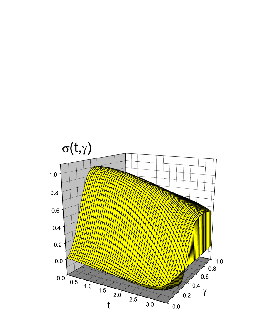
Figure 2: Anomalous average $\sigma=\sigma(t,\gamma)$ as a function of the variables $t$ and $\gamma$.

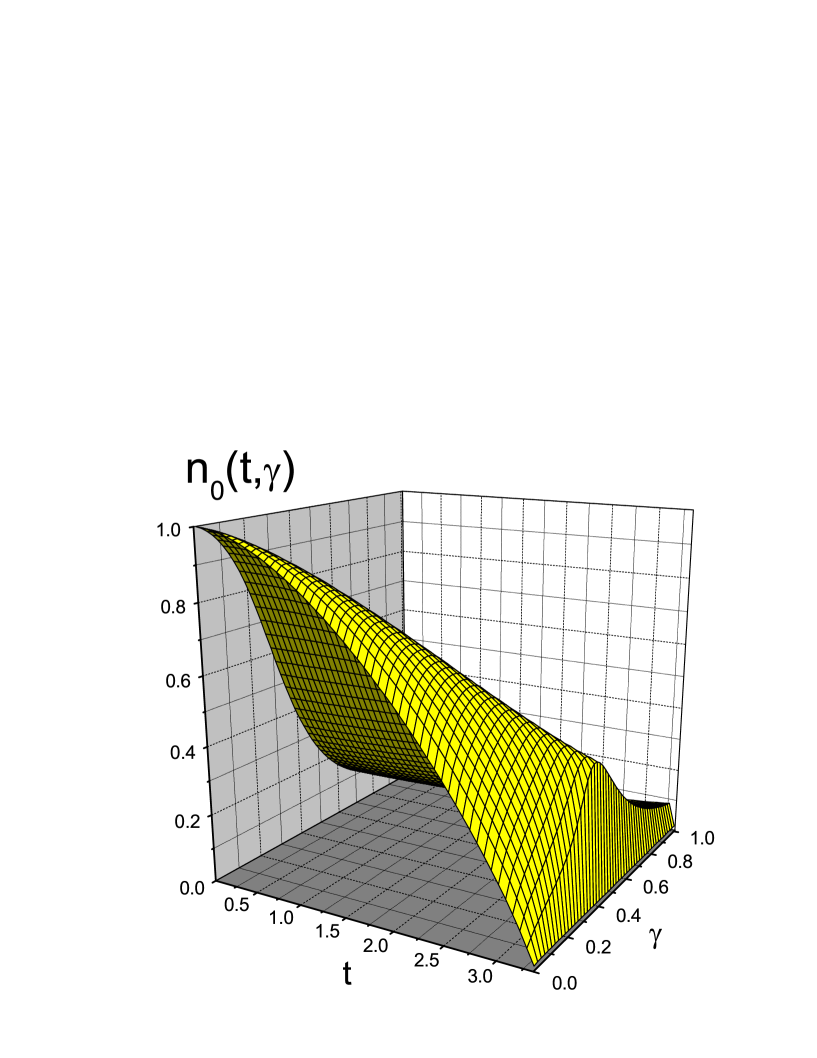
Figure 3: Condensate fraction $n_{0}=n_{0}(t,\gamma)$ as a function of the variables $t$ and $\gamma$.

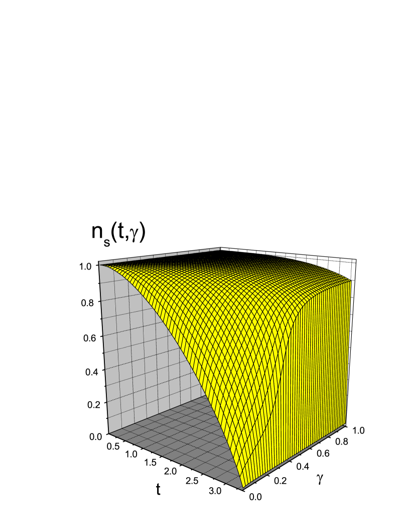
Figure 4: Superfluid fraction $n_{s}=n_{s}(t,\gamma)$ as a function of the variables $t$ and $\gamma$.

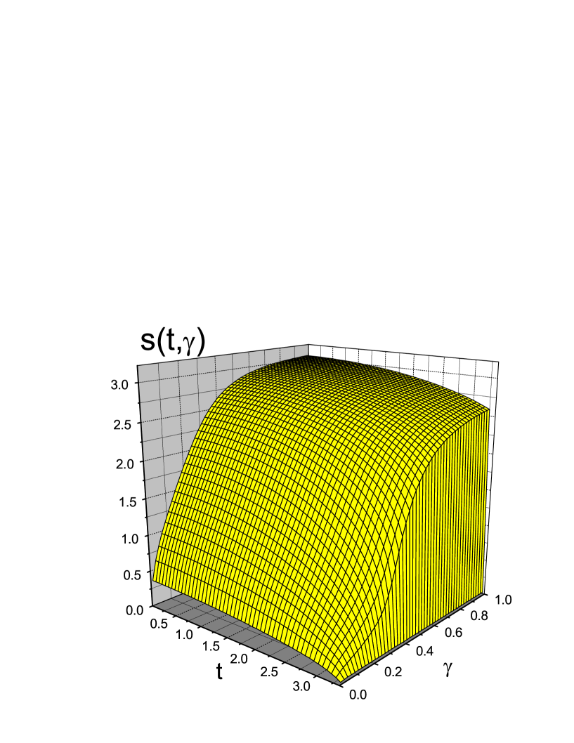
Figure 5: Dimensionless sound velocity $s=s(t,\gamma)$ as a function of temperature $t$ and the interaction strength $\gamma$.

In order to investigate the behavior of the characteristic quantities in the whole range of temperatures $t\in[0,t_{c}]$ and for arbitrary interactions $\gamma\geq 0$, we solve numerically the system of equations (42), (43), (44), and (45), together with the relation $n_{0}=1-n_{1}$. Figure 1 presents the normal fraction (43) as a function of the dimensionless temperature (39) and the interaction strength (38). In Fig. 2, we show the anomalous average (44) as a function of the same variables $t$ and $\gamma$. The condensate fraction is depicted in Fig. 3 and the superfluid fraction Fig. 4. Increasing temperature depletes both $n_{0}$ and $n_{s}$. But their dependence on the interaction strength $\gamma$ is not the same. Increasing $\gamma$ always strengthens superfluidity, and $n_{s}$ becomes larger. However the dependence of $n_{0}$ on $\gamma$ is not trivial. At zero temperature, the condensate fraction diminishes with increasing $\gamma$. But at finite temperatures, $n_{0}$, first, increases with rising $\gamma$ and then diminishes. This nonmonotonic behavior of $n_{0}$ is connected with the nonmonotonic dependence of the anomalous average $\sigma$ on $\gamma$. The dimensionless sound velocity (40), given by the solution of Eq. (42), is displayed in Fig. 5. Temperature always diminishes $s$, while interactions make $s$ larger.

5 Discussion

We have presented a detailed analysis of the condensate, $n_{0}$, and superfluid, $n_{s}$, fractions for arbitrary interactions strengths and for all temperatures in the internal $[0,T_{c}]$. The consideration is based on the self-consistent mean-field theory [20–25]. For the limiting cases of low temperatures and for those in the critical region, we derive analytic expressions for $n_{0}$ and $n_{s}$. And for the whole range of temperatures and interactions, we accomplish numerical calculations. The appearance of BEC and superfluidity occurs simultaneously at the critical temperature $T_{c}$. This transition is of second order, as it must be according to the universality theory. The superfluid fraction is practically always larger than the condensate one. They coincide only at $T_{c}$ or for the case of the ideal Bose case.

It is important to stress the crucial role of the anomalous average (44). If it would be neglected, the phase transition would be of first order, which is not correct. And, moreover, neglecting the anomalous average renders the consideration not self-consistent and the system unstable.

We may mention that the relation between the condensate and superfluid fractions can be connected with the infrared behavior of the single-particle Green function $G_{11}({\bf k},\omega)$ in the momentum-energy representation. This asymptotic behavior, having the form

$$\left|G_{11}({\bf k},0)\right|\simeq\frac{mn_{0}}{n_{s}k^{2}}\qquad(k\rightarrow 0)\;,$$

has been, first, obtained by Bogolubov, analyzed in great detail in Refs. [37], and summarized in his books [29,30]. As is evident, the Bogolubov infrared expression for $G_{11}({\bf k},0)$ can be rewritten as the limit

$$\frac{n_{0}}{n_{s}}=\lim_{k\rightarrow 0}\;\frac{k^{2}}{m}\left|G_{11}({\bf k},0)\right|\;.$$

The same asymptotic infrared expression has also been rederived and discused in Refs. [38–40]. Actually, the above relation is not an explicit definition of the ratio $n_{0}/n_{s}$ but it is an implicit equation, since $G_{11}$ itself is a complicated function of $n_{0}$. In our paper, the relation between $n_{0}$ and $n_{s}$ is given by $n_{0}=1-n_{1}$, with $n_{1}$ defined in Eq. (43), and by Eq. (45) for $n_{s}$. These equations (43) and (45) also are not the explicit expressions for $n_{0}$ and $n_{s}$, but are a part of the system of equations (42), (43), (44), and (45). Solving these equations makes it possible to extract the condensate and superfluid fractions as functions of temperature and interaction strength.

There is no simple general relation between the condensate and superfluid fractions, represented as explicit functions of temperature and gas parameter. In some limiting cases, it is possible to find asymptotic relations between these functions. For example, at low temperature, the fractions are related through Eq. (50). When, in addition, the interaction is asymptotically weak, satisfying Eq. (60), then both these fractions are close to each other, as in Eqs. (62), (63), and (64).

In the opposite case, when temperatures are low, but the interaction is strong, the condensate fraction is drastically depleted, in agreement with Eq. (68). At the same time, the superfluid fraction, according to Eq. (69), is close to one. The limiting case, corresponding to Eq. (70), could be realized in low-temperature experiments with cold atoms by increasing their scattering length by means of the Feshbach-resonance techniques. Then the state of the Bose gas can be achieved, which contains a very small condensate fraction, though being almost completely superfluid.

Another way of creating the state with a tiny condensate fraction, but with a large superfluid fraction, close to one, could be by loading atoms into an optical lattice, so that to reduce their effective mass. Diminishing the effective mass, as follows from Eq. (7), is equivalent to the increase of the effective interaction. In the one-dimensional case, the strengthening of atomic interactions would result in the effective fermionization of bosons, corresponding to the Girardeau mapping (see review article [7]).

The analysis of the present paper can be straightforwardly extended to nonuniform systems, such as atomic systems in trapping potentials. For shallow traps, the local-density approximation (see Refs. [2.3]) can be employed. Then the overall consideration remains practically the same as above, merely with the appearing dependence on the real-space variable. In that case, the equations of the present paper can be interpreted as being written for the center of the trap.

In the general case of an arbitrary trapping potential, we again could follow the same steps as above, just with some technical complications, caused by the system nonuniformity [20-22, 32]. Then the main difference is that the Hartree-Fock-Bogolubov decoupling for the field operators of uncondensed atoms should be done in the real-space representation and the general form of the Bogolubov canonical transformations [29, 30] has to be used, as in Ref. [32]. Following this way for atoms in a trap with a trapping potential $U({\bf r})$ and local interactions $\Phi({\bf r})=\Phi_{0}\delta({\bf r})$, we can use the Hartree-Fock-Bogolubov approximation for a nonuniform matter and the canonical transformations as in Ref. [32]. Then, introducing the notation

$$\omega({\bf r})=-\;\frac{\nabla^{2}}{2m}+U({\bf r})+2\Phi_{0}\rho({\bf r})-\mu_{1}\;,$$

$$\Delta({\bf r})=\Phi_{0}\left[\rho_{0}({\bf r})+\sigma_{1}({\bf r})\right]\;,$$

where the total density of atoms is the sum of the density of condensed and uncondensed atoms,

$$\rho({\bf r})=\rho_{0}({\bf r})+\rho_{1}({\bf r})\;,$$

we obtain the Bogolubov equations, providing the diagonalization of the Hamiltonian,

$$\omega({\bf r})u_{k}({\bf r})+\Delta({\bf r})v_{k}({\bf r})=\varepsilon_{k}u_{k}({\bf r})\;,\qquad\omega^{*}({\bf r})v_{k}({\bf r})+\Delta^{*}({\bf r})u_{k}({\bf r})=-\varepsilon_{k}v_{k}({\bf r})\;.$$

Here $k$ is a multi-index labelling the solutions to the above eigenproblem. Since $\omega({\bf r})$ is real, we can take $\Delta({\bf r})$ to be also real. The Bogolubov equations define the spectrum of collective excitations and the coefficient functions $u_{k}({\bf r})$ and $v_{k}({\bf r})$. The latter functions have to satisfy the canonical conditions, similar to the uniform case, which would guarantee the Bose commutation relations of the field operators. Note that the anomalous average in these equations cannot be omitted, since, as has been shown above, the anomalous average is of the order of the normal average. Omitting the anomalous average would lead to incorrect results.

The space-dependent condensate density

$$\rho_{0}({\bf r})=|\eta({\bf r})|^{2}\;$$

is defined through the condensate wave function $\eta({\bf r})$, satisfying the equation

$$\left[-\;\frac{\nabla^{2}}{2m}+U({\bf r})\right]\eta({\bf r})+\Phi_{0}\left[|\eta({\bf r})|^{2}\eta({\bf r})+2\rho_{1}({\bf r})\eta({\bf r})+\sigma_{1}({\bf r})\eta^{*}({\bf r})\right]=\mu_{0}\eta({\bf r})\;.$$

If $\Delta({\bf r})$ is real, then $\sigma_{1}({\bf r})$ is also real. For an equilibrium system, the condensate function $\eta({\bf r})$ is real. The parameter $\mu_{0}$ is given by the normalization condition

$$N_{0}=\int|\eta({\bf r})|^{2}\;d{\bf r}\;.$$

The normal and anomalous averages, $\rho_{1}({\bf r})$ and $\sigma_{1}({\bf r})$, are defined in the standard way. The number of uncondensed atoms is

$$N_{1}=\int\rho_{1}({\bf r})\;d{\bf r}\;.$$

The condition of the condensate existence

$$\min_{k}\varepsilon_{k}=0\;,\qquad\varepsilon_{k}\geq 0\;,$$

gives $\mu_{1}=\mu_{1}(T)$ as a function of temperature and other system parameters, such as the gas parameter. Hence, the number of uncondensed atoms, $N_{1}=N_{1}(T)$, is also a function of temperature and all other system parameters, As as result, we can find the number of condensed atoms $N_{0}=N_{0}(T)$ as $N_{0}(T)=N-N_{1}(T)$ and, respectively, the condensate fraction $N_{0}/N$.

Thus, the whole procedure for trapped atoms is ideologically the same as for the uniform system. The technical complications come from the necessity to solve the equation for the condensate function and the Bogolubov equations for the coefficient functions and the collective spectrum. This, generally, requires the usage of extensive numerical calculations.

Figure Captions

Fig. 1. Fraction of uncondensed atoms $n_{1}=n_{1}(t,\gamma)$ as a function of the dimensionless temperature $t$ and of the interaction strength $\gamma$.

Fig. 2. Anomalous average $\sigma=\sigma(t,\gamma)$ as a function of the variables $t$ and $\gamma$.

Fig. 3. Condensate fraction $n_{0}=n_{0}(t,\gamma)$ as a function of the variables $t$ and $\gamma$.

Fig. 4. Superfluid fraction $n_{s}=n_{s}(t,\gamma)$ as a function of the variables $t$ and $\gamma$.

Fig. 5. Dimensionless sound velocity $s=s(t,\gamma)$ as a function of temperature $t$ and the interaction strength $\gamma$.

References

- [1] A.S. Parkins and D.F. Walls, Phys. Rep. 303, 1 (1998).
- [2] P.W. Courteille, V.S. Bagnato, and V.I. Yukalov, Laser Phys. 11, 659 (2001).
- [3] L. Pitaevskii and S. Stringari, Bose-Einstein Condensation (Clarendon, Oxford, 2003).
- [4] V.I. Yukalov, Laser Phys. Lett. 1, 435 (2004).
- [5] J.O. Andersen, Rev. Mod. Phys. 76, 599 (2004).
- [6] K. Bongs and K. Sengstock, Rep. Prog. Phys. 67, 907 (2004).
- [7] V.I. Yukalov and M.D. Girardeau, Laser Phys. Lett. 2, 375 (2005).
- [8] N.N. Bogolubov, J. Phys. (Moscow) 11, 23 (1947).
- [9] N.N. Bogolubov, Moscow Univ. Phys. Bull. 7, 43 (1947).
- [10] W.H. Keesom, Helium (North-Holland, Amsterdam, 1942).
- [11] K. Mendelssohn, Cryophysics (Interscience, New York, 1960).
- [12] I.M. Khalatnikov, Theory of Superfluidity (Nauka, Moscow, 1971).
- [13] S.J. Putterman, Superfluid Hydrodynamics (North-Holland, Amsterdam, 1974).
- [14] F.H. Wirth and R.B. Hallock, Phys. Rev. B 35, 89 (1987).
- [15] T.R. Sosnick, W.M. Snow, and P.E. Sokol, Phys. Rev. B 41, 11185 (1990).
- [16] E.I. Pollock and D.M. Ceperley, Phys. Rev. B 36, 8343 (1987).
- [17] D.M. Ceperley, Rev. Mod. Phys. 67, 279 (1995).
- [18] E. Timmermans, P. Tommasini, M. Hussein, and A. Kerman, Phys. Rep. 315, 199 (1999).
- [19] R.A. Duine and H.T.C. Stoof, Phys. Rep. 396, 115 (2004).
- [20] V.I. Yukalov, Phys. Rev. E 72, 066119 (2005).
- [21] V.I. Yukalov, Phys. Lett. A 359, 712 (2006).
- [22] V.I. Yukalov, Laser Phys. Lett. 3, 406 (2006).
- [23] V.I. Yukalov and H. Kleinert, Phys. Rev. A 73, 063612 (2006).
- [24] V.I. Yukalov and E.P. Yukalova, Phys. Rev. A 74, 063623 (2006).
- [25] V.I. Yukalov and R. Graham, Phys. Rev. A 75, 023619 (2007).
- [26] G. Roepstorff, J. Stat. Phys. 18, 191 (1978).
- [27] E.H. Lieb, R. Seiringer, and J. Yngvason, Phys. Rev. Lett. 94, 080401 (2005).
- [28] E.H. Lieb, R. Seiringer, J.P. Solovej, and J. Yngvason, The Mathematics of the Bose Gas and Its Condensation (Birkhauser, Basel, 2005).
- [29] N.N. Bogolubov, Lectures on Quantum Statistics (Gordon and Breach, New York, 1967), Vol. 1.
- [30] N.N. Bogolubov, Lectures on Quantum Statistics (Gordon and Breach, New York, 1970), Vol. 2.
- [31] V.I. Yukalov and E.P. Yukalova, Laser Phys. Lett. 2, 506 (2005).
- [32] V.I. Yukalov, Laser Phys. 16, 511 (2006).
- [33] H. Kleinert, Path Integrals (World Scientific, Singapore, 2004).
- [34] T.D. Lee and C.N. Yang, Phys. Rev. 112, 1419 (1958).
- [35] E. Burovski, J. Machta, N. Prokofiev, and B. Svistunov, Phys. Rev. B 74, 132502 (2006).
- [36] J.O. Andersen, Phys. Rev. D 75, 065011 (2007).
- [37] N.N. Bogolubov, Preprint JINR D-781 (1961); Preprint JINR P-1395 (1963); Preprint JINR P-1451 (1963).
- [38] B.D. Josephson, Phys. Lett. 21, 608 (1966).
- [39] V.N. Popov, Functional Integrals in Quantum Field Theory and Statistical Physics (Reidel, Dordrecht, 1983).
- [40] M. Holzmann and G. Baym, e-print cond-mat/0703755 (2007).