Where are the edge-states near the quantum point contacts?
A self-consistent approach.

Abstract

In this work, we calculate the current distribution, in the close vicinity of the quantum point contacts (QPCs), taking into account the Coulomb interaction. In the first step, we calculate the bare confinement potential of a generic QPC and, in the presence of a perpendicular magnetic field, obtain the positions of the incompressible edge states (IES) taking into account electron-electron interaction within the Thomas-Fermi theory of screening. Using a local version of the Ohm’s law, together with a relevant conductivity model, we also calculate the current distribution. We observe that, the imposed external current is confined locally into the incompressible strips. Our calculations demonstrate that, the inclusion of the electron-electron interaction, strongly changes the general picture of the transport through the QPCs.

1 Introduction

At low temperatures, low-dimensional electron systems manifest peculiar quantum-transport properties. One of the key elements of such transport systems are the quantum point contacts (QPC) constructed on a two-dimensional electron system (2DES). The wide variety of the experiments concerning QPCs  [1], including quantum Hall effect (QHE) based Mach-Zehnder interferometer (MZI) [2, 3], have attracted many theoreticians to investigate their electrostatic [4] and transport properties [5, 6]. However, a realistic modelling of QPCs that also takes into account the involved interaction effects is still under debate. The magneto-transport properties of such narrow constrictions is typically based on the standard 1DES [7], which relates the conductance through the structure to its scattering characteristics, considering typically a hard-wall confinement potential. The reliability of such non-interacting approaches is limited, since interactions are inevitable in many cases and plays a major role in determining the electronic and transport properties. In order to account for the interactions simplified models are used with some phenomenological parameters, which is not always evident whether such a description is sufficient to reproduce the essential physics.

The QHE based MZI [2] has become a central interest to the community, since it provides the possibility to infer interaction mechanisms and dephasing [8, 9] between the ES by achieving extreme contrast interference oscillations. In these experiments ESs [7, 10, 11, 12] are assumed to behave like optical beams, whereas QPCs simulate the semi-transparent mirror in its optical counterpart. The unexpected behavior of interfering electrons, such as path-length-independent visibility oscillations, is believed to be related to long range $e-e$ interactions. Thus, the experimental findings present a clear demonstration of the breakdown of, commonly used, Landauer’s conductance picture away from the linear regime. Here, we calculate the effective potential in a self-consistent manner and , in addition, using a local version of the Ohm’s law within and out-of-the-linear-response regime, we obtain the current distribution near the QPC’s. We essentially show that, in the presence of an IES, the imposed current is confined to this region, otherwise is distributed classically.

2 Model, Results and Discussion

Our aim is to calculate the distribution of the ES within a interacting model. We start with the bare confinement potential obtained from the lithographically defined construction, following Ref’s [4, 13]. For a given pattern of (metallic) gates residing on the surface and the potential values $V_{\rm g}(x,y,0)$, one can obtain the potential experienced $V_{\rm ext}(x,y)$ by the 2DES beneath using semi-analytical scheme [13] yielding

$$V_{\rm{ext}}({\bf{r}},z)=\frac{1}{\kappa}\int{\frac{|z|}{2\pi(z^{2}+|{\bf{r}}-{\bf{r^{\prime}}}|^{2})^{3/2}}}V_{\rm g}({\bf{r^{\prime}}},0)d{\bf{r^{\prime}}},$$ (1)

where $\kappa$ is the dielectric constant of the hetero-structure ($\approx 12.4$ for GaAs/AlGaAs) and ${\bf{r}}=(x,y)$. Given the external potential in the position space, it is straight forward to calculate the screened potential in the momentum space $(q)$ by $V_{\rm scr}(q)=V_{\rm ext}(q)/\epsilon(q)$ using the Thomas-Fermi dielectric function, $\epsilon(q)=1+1/(a_{0}|q|)$, where $a_{0}/2=a^{\star}_{B}=\bar{\kappa}\hbar^{2}/(me^{2})$ (for GaAs $a_{\rm B}^{\star}=9.8\,$nm). We use this potential to initialize the self-consistent scheme described below, to obtain density $n_{\rm el}(\bf{r})$ and potential distribution in the presence of a perpendicular magnetic field, $B$, at a finite temperature $T$, $\mu^{\star}({\bf{r}})$ is SC’ly found. In the absence of an fixed external current $I$, $\mu^{\star}({\bf{r}})$ is position independent and is constant all over the sample, which is in turn determined by the average electron (surface) number density, $\bar{n_{\rm el}}({\bf{r}})$. In our calculations we set $\overline{n}_{\rm el}=3.0\cdot 10^{11}$ cm^-2, corresponding to a Fermi energy $E_{\rm F}\sim 10.7$ meV. Starting from $V_{\rm scr}({\bf{r}})$ one can obtain the electron density distribution, within the Thomas-Fermi approximation [14] (TFA), from

$$n_{\rm el}({\bf{r}})=\int dE\,D(E)f\big{(}[E+V({\bf{r}})-\mu^{\star}]/k_{B}T\big{)},$$ (2)

where $D(E)$ is the Gaussian broadened (single-particle) density of states (DOS) and $f(\xi)=[1+e^{\xi}]^{-1}$ the Fermi function. The total potential energy of an electron, $V({\bf{r}})=V_{\rm ext}({\bf{r}})+V_{H}({\bf{r}})$, differs from the Hartree potential energy $V_{H}({\bf{r}})$ by the contribution due to external potentials and is calculated from

$$V({\bf{r}})=V_{\rm ext}({\bf{r}})+\frac{2e^{2}}{\bar{\kappa}}\int_{A}\!d{\bf{r^{\prime}}}K({\bf{r}},{\bf{r^{\prime}}})\,n_{\rm el}({\bf{r^{\prime}}}).$$ (3)

For periodic boundary conditions, the kernel $K({\bf{r}},{\bf{r^{\prime}}})$ can be found in a well known text book  [15], otherwise has to be solved numerically.

In a classical manner, if a current is driven in $y$ direction in the presence of a perpendicular $B$ field a Hall potential develops in the $x$ direction. Therefore the electrochemical potential has to be modified due to external field in the $y$ direction with $E(\textbf{r})=\nabla\mu^{\star}(\textbf{r})/e=\hat{\rho}(\textbf{r})j(\textbf{r})$, for a given resistivity tensor and boundary conditions, in the thermal-equilibrium (locally), which brings a new self-consistent loop to our problem. We calculate the electric field by solving the equation of continuity under static conditions, $\nabla.j({\bf{r}})=0$, and $\nabla\times E({\bf{r}})=0$, for a fixed total current, self-consistently.

As mentioned above, in the single particle model it is believed that the current is carried by the ballistic 1D Landauer-Büttiker (LB)-ES and the conductance is obtained by the transmission coefficients. Here we calculate, the electron and current density self-consistently and observe the different distributions of the IES under quantum Hall conditions, within the linear response regime. We will always consider the case, where $E_{F}$ is larger than the hight of the barrier at the center of the QPC, so that the conductance is finite and it is at least equal to the first Landau energy ($\Omega/2=\hbar\omega_{c}/2)=eB/2m$). In Fig. 1, we selected three representative $B$ field values, such that (i) the system is almost compressible (a); (ii) the IES merge at the opening of the QPC (b) and; (iii) the IES percolate through the constraint (c). From the ”classical” current point of view we observe that, the current biased from bottom is (almost) homogeneously distributed all over the sample if there exists no IES inside the constraint, the current passes through the QPC and ends at the right top contact, mostly (d). Fig. 1e, shows us that, the current is confined to the IES and conductance is quantized, whereas for $\Omega=1.4$ it is a bit larger than $e^{2}/h$. These results indicate that, the ESs present structures inside the QPCs if one models them in a more realistic scheme rather than as a single point, although the conductance quantization remains unaffected. Since now we can calculate the widths of the IES, depending on the magnetic field and sample structure it is also possible within this model to obtain the electron velocity inside IES, which may be combined with a recent work by I. Neder [16]. This work is based on non-Gaussian noise measurements at the Mach-Zehnder interference experiments. Their main finding is that the unexpected visibility oscillations observed, can be explained by the interaction between the ”detector” and ”interference” edge channels. The essential parameters of this work are the electron velocity at the detector edge channel and the coupling (interaction) strength between the detector and the interference channels. We believe that, an extension of our present model to a realistic system may contribute to the understanding of the mentioned experiments.

We would like to thank R. R. Gerhardts for his fruitful lectures on screening theory, enabling us to understand the basics. The authors acknowledge the support of the Marmaris Institute of Theoretical and Applied Physics (ITAP), TUBITAK grant $105T110$, TUBAP-739-754-759, SFB631 and DIP.

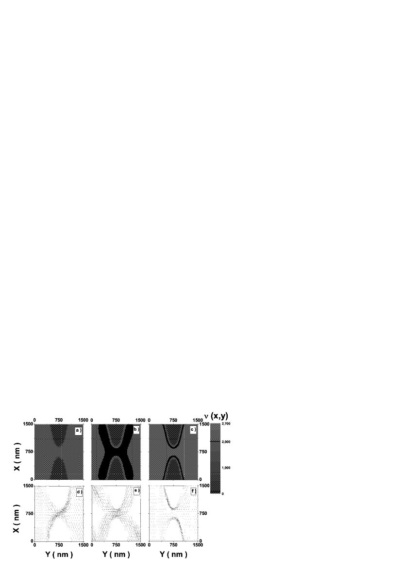
Figure 1: The color coded $\nu(x,y)$ for $\Omega=1.4,1.24,1.13$ (a-c) and corresponding current distribution indicated by the arrows. The calculations are done at $\Omega/k_{B}T\approx 0.025$ for a fixed external current driven in the $y$ direction ($j({\bf r})=j_{0}(0,0.1)$), where the 1D current density is set to $-0.42\times 10^{-2}$ A/m. The gates defining the QPC, are taken to be $300$ nm apart and biased with $-0.3$ V. The 2DES is $85$ nm below the surface and unit cell is a square with dimensions $1500\times 1500$ nm².

References

- [1] D. A. Wharam et al, J. Phys. C 21, (1988). B. J. van Wees et al, Phys. Rev. Lett 60, 848 (1988). K. J. Thomas at al, Phys. Rev. Lett. 77, 135 (1996). V. Khrapai, S. Ludwig, J. Kotthaus and W. Wegscheider, cond-mat/0606377.
- [2] Y. Ji, Y. Chung, D. Sprinzak, M. Heiblum, D. Mahalu and H. Shtrikman, Nature 422, 415 (2003).
- [3] I. Neder, M. Heiblum, Y. Levinson, D. Mahalu and V. Umansky, Phys. Rev. Lett. 96, 016804 (2006).
- [4] A. Siddiki and F. Marquardt, Phys. Rev. B 75, 045325 (2007).
- [5] Y. Meir, K. Hirose and N. S. Wingreen, Phys. Rev. Lett. 89, 196802 (2002). T. Rejec and Y. Meir, Nature 442, 900 (2006).
- [6] S. Ihnatsenka and I. V. Zozoulenko, ArXiv Condensed Matter e-prints (2007).
- [7] M. Büttiker, IBM J. Res. Dev. 32, 317 (1988).
- [8] F. Marquardt and C. Bruder, Phys. Rev. Lett. 92, 056805 (2004).
- [9] P. Samuelsson, E. Sukhorukov and M. Buttiker, Phys. Rev. Lett. 92, 026805 (2004).
- [10] D. B. Chklovskii, B. I. Shklovskii and L. I. Glazman, Phys. Rev. B 46, 4026 (1992).
- [11] A. Siddiki and R. R. Gerhardts, Phys. Rev. B 70, 195335 (2004).
- [12] I. V. Zozoulenko and M. Evaldsson, Appl. Phys. Lett. 85, 3136 (2004).
- [13] J. H. Davies and I. A. Larkin, Phys. Rev. B 49, 4800 (1994).
- [14] J. H. Oh and R. R. Gerhardts, Phys. Rev. B 56, 13519 (1997).
- [15] P. M. Morse and H. Feshbach, Methods of Theoretical Physics (McGraw-Hill, New York, 1953), Band II, p. 1240.
- [16] I. Neder and F. Marquardt, New Journal of Physics 9, 112 (2007).