Intrinsic optical bistability of thin films of linear molecular aggregates: The one-exciton approximation

Abstract

We perform a theoretical study of the nonlinear optical response of an ultrathin film consisting of oriented linear aggregates. A single aggregate is described by a Frenkel exciton Hamiltonian with uncorrelated on-site disorder. The exciton wavefunctions and energies are found exactly by numerically diagonalizing the Hamiltonian. The principal restriction we impose is that only the optical transitions between the ground state and optically dominant states of the one-exciton manifold are considered, whereas transitions to other states, including those of higher exciton manifolds, are neglected. The optical dynamics of the system is treated within the framework of truncated optical Maxwell-Bloch equations in which the electric polarization is calculated by using a joint distribution of the transition frequency and the transition dipole moment of the optically dominant states. This function contains all the statistical information about these two quantities that govern the optical response, and is obtained numerically by sampling many disorder realizations. We derive a steady-state equation that establishes a relationship between the output and input intensities of the electric field and show that within a certain range of the parameter space this equation exhibits a three-valued solution for the output field. A time-domain analysis is employed to investigate the stability of different branches of the three-valued solutions and to get insight into switching times. We discuss the possibility to experimentally verify the bistable behavior.

I Introduction

Optical circuits make use of light to process information. They operate at the speed of light with almost no energy dissipation, unlike electronic analogs. Optical fibres Mollenauer80 ; Hasegawa95 and photonic crystal fibers Russel03 have already found important applications in optical communications and optoelectronic devices. Implementing ultrafast optical sources and all-optical switches based on novel (quantum-confined) materials, such as organic thin films and quantum dots, Wada04 as well as silicon-based structures, Almeida04 is now in progress. The realizability of a single-photon optical switch based on warm rubidium vapor has recently been demonstrated. Dawes05

A key element of any optical logic device is the optical switch, which either passes or reflects the incoming light, depending on its intensity. One possibility to design an optical switch is to utilize the phenomenon of optical bistability. Since the theoretical prediction of this effect by McCall McCall74 and its experimental demonstration by Gibbs, McCall, and Venkatesan Gibbs76 for a cavity filled with potassium atoms, an extensive literature, both theoretical and experimental, has developed on this topic (see Refs. Abraham82, ; Lugiato84, ; Gibbs85, for historical overviews and Ref. Rosanov96, for recent developments on optical instability in wide aperture laser systems). A generic optical bistable element exhibits two stable stationary transmission states for the same input intensity, a property which in principle opens the door to applications such as all-optical switches, optical transistors, and optical memories.

Nonlinearity and feedback are the two necessary ingredients in order to enable optical bistable response of an optical system. The former can be provided, e.g., by a saturable medium, while a cavity (mirrors) can serve to build up a feedback. This arrangement has been used in the first demonstration of controlling light with light. Gibbs76 Sometimes, however, the nonlinearity itself plays the role of the feedback. Here, bistability is an intrinsic property of the material; no external feedback, like a cavity, is needed. Thus, mirrorless (or cavityless) optical bistability can be realized, which is even more advantageous from the viewpoint of designing all-optical devices. During the past decade, this type of bistability has been observed in a variety of inorganic materials heavily doped with rare-earth ions. Hehlen94 ; Gamelin00 ; Noginov01 ; Goldner04 In Refs. Hehlen94, , a population dependent dipole-dipole interaction in ion pairs has been put forward as a nonlinearity and feedback mechanism to explain the effect. This interpretation has been debated in a number of papers. Bodenschatz96 ; Guillot-Noel01 ; Malyshev98 ; Gamelin00 ; Noginov01 ; Goldner04 ; Ciccarello03

Another class of materials, promising from the viewpoint of all-optical manipulation of light, are molecular aggregates and conjugated polymers. These systems commonly exhibit narrow absorption bands and suppression of exciton-phonon coupling, superradiance and giant optical nonlinearities, fast collective optical response and efficient energy or charge transport (see for an overview Refs. Spano94, ; Kobayashi96, ; Hadzii99, ; vanAmerongen00, ; Knoester02, ; Spano06, ; Scholes06, ), which are ingredients necessary to design optoelectronics or all-optical devices. Molecular aggregates and conjugated polymers have already been used to fabricate light emitting diodes Greenham93 and organic solid-state lasers. Kranzelbinder00

One particularly interesting effect, which has already received a considerable amount of theoretical discussion, but still awaits experimental realization, is the mirrorless optical bistability of a single molecular aggregate Malyshev96 or an assembly of molecular aggregates. Malyshev00 ; Jarque01 ; Glaeske01 The bistable behavior of a single linear aggregate consists of a sudden switching of the aggregate’s excited state population from a low level to a higher one upon a small change of the input intensity around a critical point. The effect originates from a dynamic resonance frequency shift, which depends on the number of excited monomers in the aggregate. The origin of this shift lies in the quasi-fermionic nature of Frenkel excitons in one dimension. Chesnut63 ; Agranovich68 ; Spano91 This nonlinearity plays the role of intrinsic feedback, necessary for bistability to occur. There exists, however, a restriction on the aggregate length: an aggregate exhibits bistable behavior only if its coherence length is larger than the emission wavelength, which makes experimental realization problematic.

An assembly of molecular aggregates arranged in an ultrathin film geometry (with the film thickness small compared to the emission wavelength) may display intrinsic optical bistability governed by another mechanism, where the density of molecules becomes the driving parameter. The same mechanism holds for an ultrathin film of homogeneously broadened two-level systems. Zakharov88 When the density in the film is high enough, the on-resonance refractive index can get sufficiently large to totally reflect an incoming field of low intensity. Then the incoming field is almost completely compensated by a secondary field of opposite phase, which is generated by the aggregate dipoles. The dipole-induced field is bounded in magnitude, meaning that this picture only holds if the incoming field intensity is smaller than a certain value, determined by the density of aggregates. When this value is exceeded, the aggregates become saturated, which suppresses the dipole-induced field and abruptly changes the (nonlinear) refractive index and transmittivity of the film. The field produced by the aggregate dipoles plays the role of intrinsic feedback. The output field depends nonlinearly on the input field of the film.

In Refs. Malyshev00,  - Glaeske01, a thin film arrangement of oriented linear J-aggregates was considered, where the localization segments of a single disordered aggregate were modeled as independent homogeneous chains of fluctuating size. Each segment was considered as a few-level system, with an individual ground state and one or two excited states corresponding to the dominant optical states of the segment. Within this framework, both the ground state to one-exciton Malyshev00 and one-to-two Glaeske01 exciton transitions were taken into account, and bistable behavior was found in a certain region in the parameter space.

The approach used in Refs. Malyshev00, and Glaeske01, assumed full correlation of fluctuations of the lowest exciton energy and the transition dipole moment, taking both magnitudes as solely depending on the segment size. The real picture, however, is quite different. Malyshev95 ; Malyshev01 In practise the optical response of J-aggregates is strongly affected by disorder in the molecular transition energies. The band-edge of the exciton energy spectrum of such a disordered aggregate is formed by states that are localized on segments with small overlap. The lowest state of a segment is optically dominant, whereas the other states have a much smaller oscillator strength. The energy of the lowest state is not correlated with the size of the segment; it is determined by uncorrelated well-like fluctuations of the site potential. Lifshits68 Therefore, the optically dominant states of non-overlapping segments can be arbitrarily close in energy, having at the same time completely different transition dipoles. Bednarz04 In other words, the transition dipoles and energies of the relevant states turn out to be uncorrelated rather than correlated.

In this paper, we exploit the two-level model, implemented in Refs. Malyshev00, and Jarque01, , to describe the film’s optical response. However, unlike Refs. Malyshev00, and Jarque01, , we will account properly for the statistical fluctuations of the transition dipole moment and the transition energy, as they appear after diagonalizing the Frenkel exciton Hamiltonian with uncorrelated on-site disorder. We calculate the joint probability distribution of these quantities and use it to compute the electric polarization of the film, which features in the Maxwell equation for the field. The aggregate segment dynamics is described within the $2\times 2$-density matrix formalism. We derive a novel steady-state equation for the output field intensity as a function of the input intensity in terms of the joint probability distribution of the energy and the transition dipole moment. On this basis, the bistability phase diagram of the film is calculated. The critical parameter for bistability to occur turns out to be different (larger) than that found in Refs. Malyshev00, . By numerically solving the truncated Maxwell-Bloch equations in the time domain, we study the stability of the different branches of the three-valued solution for the output field intensity. The calculation of an optical hysteresis loop (an adiabatic up-and-down-scan of the field) demonstrates that only two of them are stable. A new element in the paper is that we also analyze switching time between both stable branches, and show that it slows down dramatically close to the switching point.

The outline of this paper is as follows. In section II we present the model and mathematical formalism. Section III deals with the linear regime of the transmission. The steady state equation for the output intensity in the nonlinear regime is derived in Sec. IV. In Sec. V, the stability of different branches is considered, together with a study of the switching time. In Sec. VI we discuss the possibility to achieve optical bistability using J-aggregates of polymethine dyes. Section VII summarizes the paper. Finally, in the Appendix we address the effect of interference of the ground state to one-exciton transitions, originating from the fact that excitons are born from the same ground state, with all monomers being unexcited.

II Model and formalism

We aim to study the transmittivity of an assembly of linear J-aggregates arranged in a thin film geometry (with the film thickness $L$ small compared to the emission wavelength $\lambda^{\prime}$ inside the film). All aggregates are aligned in one direction, parallel to the film plane. Such an arrangement can be achieved, e.g., by spin-coating. Misawa93 The limit of $L\ll\lambda^{\prime}$ allows one to neglect the inhomogeneity of the field inside the film. The aggregates in the film are assumed to be decoupled from each other. This finds its justification in the strongly anisotropic nature of the system we have in mind. As we will see later (Sec. VI), films of interest for bistability should have a molecular density of the order of $10^{19}$ cm^-3. With a typical separation of 1 nm between molecules within a single aggregate, this implies that neighboring aggregates are separated by 10 nm. Thus, the dominant dipole-dipole interactions between molecules of different chains are a factor of 1000 weaker than those within chains. As a consequence, we expect that the former interactions will merely result in small shifts of resonance energies, away from the single-chain exciton energies considered below.

On the other hand, the effect of interactions of the aggregate molecules with the surrounding host molecules is important, because as a consequence of the usually inhomogeneous nature of the host media, they lead to disorder in the molecular transition energies and in the molecular transfer integrals, both of which give rise to localization of the exciton states on segments of the aggregates. Finally, thermal fluctuations in the environment result in intraband scattering of the excitons that causes two effects: equilibration of the exciton population and homogeneous broadening of the exciton levels. In this paper, we neglect the former effect. This finds its justification in many experimental studies, which have shown that the fluorescence Stokes shift of J-aggregates of cyanine dyes usually is very small. Fidder90 ; Minoshima94 ; Moll95 ; Kamalov96 )

II.1 A single aggregate

We model a single aggregate as a linear array of $N$ two-level monomers with parallel transition dipoles. In this paper, we restrict ourselves to optical transitions between the ground state an the one-exciton manifold, described by the Frenkel exciton Hamiltonian

$$H_{0}=\sum_{n=1}^{N}\>\epsilon_{n}|n\rangle\langle n|+\sum_{n,m}^{N}\>J_{nm}\>|n\rangle\langle m|\ ,$$ (1)

where $|n\rangle$ denotes the state in which the $n$th site is excited and all the other sites are in the ground state and $\epsilon_{n}$ is the excitation energy of site $n$. The $\epsilon_{n}$ are taken at random and uncorrelated from each other from a Gaussian distribution with mean $\epsilon_{0}$ (the excitation energy of an isolated monomer) and standard deviation $\sigma$. The transfer interactions $J_{nm}$ are considered to be of dipolar origin and non fluctuating: $J_{nm}=-J/|n-m|^{3}$   $(J_{nn}\equiv 0)$. Here the parameter $J$ represents the nearest-neighbor transfer interaction, which will be chosen positive (as is appropriate for J-aggregates). The exciton energies $\varepsilon_{\nu}$ ($\nu=1,\ldots,N$) and wavefunctions $|\nu\rangle=\sum_{n=1}^{N}\varphi_{\nu n}|n\rangle$, are obtained as eigenvalues and eigenvectors of the $N\times N$ Hamilton matrix $H_{nm}=\langle n|H|m\rangle$.

From the set of exciton states $|\nu^{\prime}\rangle$ we only take into account the optically dominant states which, for $J>0$, reside in the neighborhood of the low-energy bare band edge at $\varepsilon_{0}=\epsilon_{0}-2.404J$. These states are located at different segments of the aggregate, which overlap weakly, and have a wavefunction with no node. Therefore, they are called $s$-like states. To find all such states, we use the selection rule proposed in Ref. Malyshev01, . It reads —$\sum_{n}\varphi_{\nu n}|\varphi_{\nu n}|\big{|}>C_{0}$, where we set $C_{0}=0.8$. This rule selects states with a wavefunction consisting of mainly one peak. From now on, the state index $\nu$ will count only such $s$-like states. The number of these states is roughly equal to $N/N^{*}$, where $N^{*}$ is their typical localization size. We assume that the vibration-induced coherence length of excitons is much larger than the disorder-induced localization length, a condition that can be fulfilled at low temperature. Heijs05 In this limit, the exciton eigenstates $|\nu\rangle$ form a good basis.

The above picture implies that an aggregate is modeled as a set of independent segments, each of which has its own ground state $|0\rangle$ and an $s$-like excited state $|\nu\rangle$. The optical transition between these states is governed by the segment dipole operator $\hat{d}_{\nu}=d_{0}(|0\rangle\langle\nu|+|\nu\rangle\langle 0|)$, where $d_{0}$ is the transition dipole moment of a monomer. The corresponding transition dipole moment of a segment is calculated as $d_{\nu}=d_{0}\sum_{n}\varphi_{\nu n}\equiv d_{0}\mu_{\nu}$, where $\mu_{\nu}=\sum_{n}\varphi_{\nu n}$ is the dimensionless transition dipole moment.

The optical dynamics of a segment is described in terms of the $2\times 2$-density matrix ($\rho_{\nu\nu},\rho_{\nu 0},\rho^{*}_{\nu 0},\rho_{00}$) which obeys the Bloch-like equations (see the Appendix)

$$\dot{\rho}_{\nu\nu}=-\gamma_{\nu}\rho_{\nu\nu}+id_{\nu}\mathcal{E}\left(\rho_{0\nu}-\rho_{\nu 0}\right)\ ,$$ (2a)

$$\dot{\rho}_{\nu 0}=-\left(i\varepsilon_{\nu}+\Gamma_{\nu}\right)\rho_{\nu 0}-id_{\nu}\mathcal{E}(\rho_{\nu\nu}-\rho_{00})\ ,$$ (2b)

$$\rho_{00}+\rho_{\nu\nu}=1\ .$$ (2c)

Here we set the Plank constant $\hbar=1$ and introduced the following notations: $\gamma_{\nu}=\gamma_{0}|\mu_{\nu}|^{2}$ is the radiative rate of the exciton state $\nu$ ($\gamma_{0}$ being the monomer radiative rate), and $\Gamma_{\nu}=\frac{1}{2}\gamma_{\nu}+\gamma_{\nu 0}$ is the dephasing rate of the state $\nu$, which includes a pure dephasing term, $\gamma_{\nu 0}$. Finally, $\cal{E}$ is the total electric field inside the film (see below). Owing to the disorder, the transition energy $\varepsilon_{\nu}$, the relaxation constant $\Gamma_{\nu}$, and the transition dipole moment $\mu_{\nu}$ are stochastic variables, which differ from segment to segment. Because of the fluctuations in $\varepsilon_{\nu}$, $\Gamma_{\nu}$, and $d_{\nu}$, the density matrix elements $\rho_{\nu\nu}$, $\rho_{\nu 0}$, and $\rho_{00}$ fluctuate as well.

II.2 The Maxwell equation

In this section, we specify the field $\mathcal{E}$ which enters Eqs. (2). It consists of two contributions: the incoming field $\mathcal{E}_{i}$ and a part produced by the aggregate dipoles. The incoming field is considered to be a plane wave $\mathcal{E}_{i}=E_{i}(x,t)\cos(k_{i}x-\omega_{i}t)$ with a frequency $\omega_{i}$ and an amplitude $E_{i}(x,t)$, normally incident and polarized along the aggregate transition dipoles. Under these conditions, all the vectorial variables (transition dipole moments, incoming and outgoing fields, and the field inside the film) can be considered as scalars. The amplitude $E_{i}(x,t)$ is assumed to vary slowly on the scale of the optical period $2\pi/\omega_{i}$ and wavelength $\lambda_{i}=2\pi/k_{i}$.

We assume without loss of generality that the film is located in the ZY plane ($x=0$). Then the total field at $x=0$ (inside the film) is given by Benedict88 ; Benedict96

$$\mathcal{E}=\mathcal{E}_{i}-\frac{2\pi L}{c}\dot{\mathcal{P}}\ ,$$ (3)

where $\mathcal{P}$ is the electric polarization of the film (electric dipole moment per unit volume), the dot denotes the time derivative, and $c$ stands for speed of light. The second term in the right hand side of Eq. (3) represents the field produced by the dipoles in the film, emitted perpendicular to the film in both directions. The part propagating to the left is the reflected (plane wave) field, given at $x=0$ by $\mathcal{E}_{r}=-(2\pi L/c)\dot{\mathcal{P}}$, while the part propagating to the right is the emitted (also plane wave) field, which forms, together with the incident field $\mathcal{E}_{i}$, the transmitted signal, determined at $x=0$ by Eq. (3).

The electric polarization $\mathcal{P}$ is calculated as follows. First, we introduce the expectation value of the dipole operator of an aggregate, $d=d_{0}\sum_{\nu\in s}\>\mu_{\nu}(\rho_{\nu 0}+\rho_{0\nu})$, where the summation is performed only over the $s$-like states of the aggregate. Furthermore, this value is averaged over a physical volume $V$, containing $M$ aggregates, which, in fact, is equivalent to obtaining the average $\langle d\rangle$ over disorder realizations. After that, ${\cal P}$ is obtained by multiplying $\langle d\rangle$, with the number density $M/V$ of the aggregates. The final formula for the electric polarization reads:

$$\mathcal{P}=d_{0}n_{0}\frac{N_{s}}{N}\int d\varepsilon d\mu\,\mathcal{G}_{s}(\varepsilon,\mu)\,\mu\,[\,\rho_{10}(\varepsilon,\mu,t)+\mathrm{c.c.}]\ .$$ (4)

Here, $n_{0}=NM/V$ is the number density of monomers, $N_{s}=\Big{\langle}\sum_{\nu\in s}\>1\Big{\rangle}$ a normalization constant (having the meaning of the average number of $s$-like states in an aggregate), and $\rho_{10}(\varepsilon,\mu,t)$ is the off-diagonal density matrix element, where the indices 0 and 1 label the ground and the excited $s$-state of the segment, respectively. In our present formulation this element, as well as $\rho_{00}$ and $\rho_{11}$, are ordinary (not stochastic) functions of $\varepsilon$ and $\mu$; which formally follow from solving Eqs.(2). All stochastic aspects of the segment’s properties are taken into account through the function $\mathcal{G}_{s}(\varepsilon,\mu)$, which represents the joint probability distribution of the transition energy $\varepsilon$ and the dimensionless transition dipole moment $\mu$ of the segment. The latter is defined as

$$\mathcal{G}_{s}(\varepsilon,\mu)=\frac{1}{N_{s}}\left\langle\sum_{\nu\in s}\delta\Big{(}\varepsilon-\varepsilon_{\nu}\Big{)}\delta\Big{(}\mu-\mu_{\nu}\Big{)}\right\rangle.$$ (5)

It is worth to notice that at a given disorder strength $\sigma$, $N_{s}$ scales linearly with the aggregate size $N$. Hence, the ratio $N_{s}/N$ in Eq. (4) is $N$-independent. From our simulations we found that $N_{s}/N=0.074(\sigma/J)^{0.8}$, which nicely agrees with the disorder scaling of the typical localization size $N^{*}$. Malyshev01

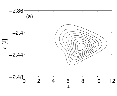
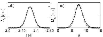
Figure 1: (a) The joint probability distribution $\mathcal{G}_{s}(\varepsilon,\mu)$ of the transition energy $\varepsilon$ and dimensionless transition dipole moment $\mu$ for $s$-like states on localization segements, obtained for a disorder strength $\sigma=0.1J$ according to Eq. (5). We used chains of length $N=500$ with the monomer transition energy $\epsilon_{0}=0$. The sampling was performed over 300 000 disorder realizations. Contour lines correspond to 10% of the peak value of the distribution. (b) - The absorption spectrum $\mathcal{A}_{s}(\varepsilon)=\int d\mu\>\mu^{2}\mathcal{G}_{s}(\varepsilon,\mu)$. (c) - The distribution $\mathcal{M}_{s}(\mu)=\int d\varepsilon\,\mathcal{G}_{s}(\varepsilon,\mu)$ of the transition dipole moment $\mu$. The solid lines represent the results of calculations, whereas the open circles are fits by a Gaussian.

After the ${\cal G}_{s}$-distribution is obtained by straightforward sampling of a sufficient number of disorder realizations, one can easily calculate the two important quantities: ${\cal A}_{s}(\varepsilon)=N_{s}^{-1}\big{\langle}\sum_{\nu\in s}\mu^{2}_{\nu}\delta\big{(}\varepsilon-\varepsilon_{\nu}\big{)}\big{\rangle}=\int d\mu\>\mu^{2}\,\mathcal{G}_{s}(\varepsilon,\mu)$, which represents the absorption spectrum, not accounting for homogeneous broadening (i.e., close to the zero-temperature spectrum), and $\mathcal{M}_{s}(\mu)=N_{s}^{-1}\big{\langle}\sum_{\nu\in s}\delta\big{(}\mu-\mu_{\nu}\big{)}\big{\rangle}=\int d\varepsilon\,\mathcal{G}_{s}(\varepsilon,\mu)$, which represents the probability density of the transition dipole moment. As we are mostly interested in the limit of dominating ingomogeneous broadening, we will refer from now on to ${\cal A}_{s}(\varepsilon)$ as to the absorption spectrum, assuming that its half width at half maximum (HWHM) $\sigma^{*}$ is larger than the homogenous HWHM (resulting from $\Gamma_{\nu}$).

An example of the distributions $\mathcal{G}_{s}(\varepsilon,\mu),{\cal A}_{s}(\varepsilon)$, and $\mathcal{M}_{s}(\mu)$ computed for an ensemble of chains with $N=500$ and a disorder strength $\sigma=0.1J$, is depicted in Fig. 1 [panels (a),(b), and (c), respectively]. Because $\mathcal{G}_{s}(\varepsilon,\mu)=\mathcal{G}_{s}(\varepsilon,-\mu)$, only $\mu>0$ is considered in the plots.

Note that in our model, the absorption spectrum $\mathcal{A}_{s}(\varepsilon)$ is almost symmetric with respect to the peak position, except the tails, which show a small asymmetry. It can be fitted well by a Gaussian, unlike the case when all the exciton states are taken into account. The latter gives rise to a Lorentzian high-energy tail of $\mathcal{A}_{s}(\varepsilon)$, reproducing the asymmetric lineshape commonly seen in experiments. The shape of the $\mathcal{M}_{s}$-distribution can also be fitted by a Gaussian, but with a lesser accuracy than the absorption spectrum. The distribution $\mathcal{G}_{s}(\varepsilon,\mu)$ exhibits interesting scaling properties with regard to the disorder strength $\sigma$. A detailed study will be presented elsewhere.

II.3 Truncated Maxwell-Bloch equations

To proceed we seek the solution of Eqs. (2) in the standard manner: we set $\rho_{10}=-(i/2)R\exp{(-i\omega_{i}t)}$ and $\mathcal{E}=(1/2)E\exp{(-i\omega_{i}t)}+\mathrm{c.c.}$, where the complex amplitudes $R$ and $E$ vary slowly on the time scale $2\pi/\omega_{i}$, and we use the rotating wave approximation. It is straightforward to arrive at a set of truncated equations for the populations $\rho_{11}$ of the one-exciton states, and the amplitudes $R$ of the off-diagonal density matrix elements, and the field $\Omega=d_{0}E$ (in frequency units):

$$\dot{\rho}_{11}=-\gamma\rho_{11}-\frac{1}{4}\mu\left(\Omega R^{*}+\Omega^{*}R\right)\ ,$$ (6a)

$$\dot{R}=-\left[i(\Delta-\Delta_{0})+\Gamma\right]R+\mu\Omega(\rho_{11}-\rho_{00})\ ,$$ (6b)

$$\Omega=\Omega_{i}+\Gamma_{R}\>\frac{N_{s}}{N}\,\int d\Delta d\mu\,\mathcal{G}(\Delta,\mu)\,\mu R\ ,$$ (6c)

where $\Delta-\Delta_{0}=\varepsilon-\omega_{i}$ is the frequency detuning between the exciton transition and the incoming field, which is decomposed into two parts: $\Delta=\varepsilon-\varepsilon_{0}$ and $\Delta_{0}=\omega_{i}-\varepsilon_{0}$ indicating, respectively, the frequency detuning of the exciton state and the incoming field from the exciton band-edge frequency $\varepsilon_{0}=\epsilon_{0}-2.404J$.

The constant $\Gamma_{R}=2\pi n_{0}{d_{0}}^{2}kL$ is an important parameter of the model. Malyshev00 ; Jarque01 ; Glaeske01 The physical meaning of $\Gamma_{R}$ can be explored by rewriting it in the form $\Gamma_{R}=\frac{3}{2\pi}\gamma_{0}n_{0}L(\lambda/2)^{2}$, where $\gamma_{0}=4d_{0}^{2}\omega^{3}/(3c^{3})$ is the monomer spontaneous emission rate and $n_{0}L$ is the surface density of monomers. The quantity $n_{0}L(\lambda/2)^{2}$ can be interpreted as the number of monomers in a $(\lambda/2)^{2}$-square that oscillate in phase. In other words, $\Gamma_{R}$ can be considered as the radiative rate of a single monomer, $\gamma_{0}$, enhanced by the number of monomers within a $(\lambda/2)^{2}$-square. Lee74 $\Gamma_{R}$ governs the Dicke superradiance of a thin film, Benedict88 ; Benedict96 as well as the collective radiative damping in the linear regime (see the next section). Therefore it is usually referred to as the superradiant constant.

The set of equations (6) together with the normalization condition (2c) and the definition (5) form the basis of our analysis. In the remainder of this paper, we will be particularly interested in the dependence of the transmitted field intensity $|\Omega|^{2}$ on the input field intensity $|\Omega_{i}|^{2}$ following from these equations.

III Linear regime

In order to get insight into the effect and interplay of the parameters that govern the bistability, we first consider the linear regime of the system. We assume that a weak input field $\Omega_{i}$ = const is switched on at $t=0$, weakness implying that the depletion of the ground state population can be neglected. Thus, we set $\rho_{00}(t)=1$ and $\rho_{11}(t)=0$, which linearizes Eqs. (6),

$$\dot{R}=-\left[i(\Delta-\Delta_{0})+\Gamma\right]R-\mu\Omega\ ,$$ (7a)

$$\Omega=\Omega_{i}+\Gamma_{R}\>\frac{N_{S}}{N}\int d\Delta d\mu\,\mathcal{G}_{s}(\Delta,\mu)\,\mu R.$$ (7b)

These equations can be solved easily in the Laplace domain. The solution for the Laplace transform of the transmitted field $\tilde{\Omega}$ reads

$$\tilde{\Omega}=\Big{[}1+\Gamma_{R}\>\frac{N_{s}}{N}\int d\Delta d\mu\,\mathcal{G}_{s}(\Delta,\mu)\,\mu^{2}$$

$$\times\frac{1}{p+\left[i(\Delta-\Delta_{0})+\Gamma\right]}\Big{]}^{-1}\>\tilde{\Omega}_{i}\ ,$$ (8)

where $p$ denotes the Laplace parameter. To evaluate this expression, we neglect the $\mu$-dependence of $\Gamma$. Then the integral over $\mu$ gives, by definition, the absorption spectrum $\mathcal{A}_{s}(\Delta)$. The latter is normalized now to $F_{s}/N_{s}$, where $F_{s}=\big{\langle}\sum_{\mu\in s}\>\mu_{\nu}^{2}\big{\rangle}$ is the average total oscillator strength of the $s$-like states per aggregate. To perform the integration over $\Delta$ explicitly, we replace $\mathcal{A}_{s}(\Delta)$ by a Lorentzian centered at $\Delta^{*}$ and with a width $\sigma^{*}$:

$$\mathcal{A}_{s}(\Delta)=\frac{F_{s}}{N_{s}}\>\frac{\sigma^{*}}{\pi}\>\frac{1}{\left[(\Delta-\Delta^{*})^{2}+{\sigma^{*}}^{2}\right]}$$ (9)

(in all our numerical results, we do not invoke this approximation and keep the exact form of the ${\cal G}_{s}$-distribution, i.e., of the absorption spectrum). With this substitution, the result of the integration over $\Delta$ reads:

$$\tilde{\Omega}=\tilde{\Omega}_{i}-\frac{\tilde{\Gamma}_{R}}{p+i(\Delta^{*}-\Delta_{0})+\Gamma+\sigma^{*}+\tilde{\Gamma}_{R}}\>\tilde{\Omega}_{i}\ ,$$ (10)

where we introduced the renormalized superradiant constant $\tilde{\Gamma}_{R}=(F_{s}/N)\Gamma_{R}$. As the total oscillator strength of $s$-like states $F_{s}<N$, the ratio $F_{s}/N<1$. We also note that $\Gamma+\sigma^{*}$ denotes the total (homogeneous plus inhomogeneous) dephasing rate.

Finally, by assuming $\Omega_{i}=\text{const}$, which corresponds to $\tilde{\Omega}_{i}=\Omega_{i}/s$ in the Laplace domain, we obtain the following time-domain behavior of the transmitted field

$$\Omega = \frac{i(\Delta^{*}-\Delta_{0})+\Gamma+\sigma^{*}}{i(\Delta^{*}-\Delta_{0})+\Gamma+\sigma^{*}+\tilde{\Gamma}_{R}}\>\Omega_{i}$$ (11)

$$+ \frac{\tilde{\Gamma}_{R}}{i(\Delta^{*}-\Delta_{0})+\Gamma+\sigma^{*}+\tilde{\Gamma}_{R}}\>\Omega_{i}$$

$$\times \exp\left[-i(\Delta^{*}-\Delta_{0})t-(\Gamma+\sigma^{*}+\tilde{\Gamma}_{R})t\right]\ .$$

As is seen from this equation, the field in the film, $\Omega$, reaches its steady-state value (given by the first term in the right-hand side) after a time $1/(\Gamma+\sigma^{*}+\tilde{\Gamma}_{R})$. If the dephasing dominates the relaxation of the dipoles, i.e., if $\Gamma+\sigma^{*}\gg\tilde{\Gamma}_{R}$, the steady state limit of the opposing dipole field, given by $-\Omega_{i}\tilde{\Gamma}_{R}/[i(\Delta^{*}-\Delta_{0})+\Gamma+\sigma^{*}+\Gamma_{R}]$, is small in magnitude compared to the incoming field $\Omega_{i}$. As a consequence, the field inside the film $\Omega\approx\Omega_{i}$. In this limit, one finds a high film transmittivity.

When $\tilde{\Gamma}_{R}\gg\Gamma+\sigma^{*}$ the superradiant damping drives the relaxation. Now the film dipoles, having sufficient time to respond collectively, can produce an opposing field $-\Omega_{i}\tilde{\Gamma}_{R}/|i(\Delta^{*}-\Delta_{0})+\Gamma+\sigma^{*}+\tilde{\Gamma}_{R}|$ of magnitude $\approx\Omega_{i}$. This field almost totally compensates the incoming field, and results in a low magnitude of the field inside the film, $|\Omega|\sim\Omega_{i}|i(\Delta^{*}-\Delta_{0})+\Gamma+\sigma^{*}|/\tilde{\Gamma}_{R}\ll\Omega_{i}$, and, consequently, in a low film transmittivity. Switching to a high transmission state now requires a field intensity $\Omega_{i}$ that saturates the system. In this case we can see optical bistable switching (see the next section).

From the above, it is clear that the interplay of superradiance and dephasing determines the linear transmittivity of the film. Hence, the ratio $\tilde{\Gamma}_{R}/(\Gamma+\sigma^{*})$ is an important parameter of the model. In the theory of bistability it is often referred to as the cooperative number. Lugiato84 ; Gibbs85

IV Steady-state analysis

IV.1 Bistability equation

In this section, we consider the steady-state regime, when we set $\Omega_{i}=\text{const}$ and $\dot{R}=\dot{\rho}_{11}=0$. It is a matter of simple algebra to derive the following equation for the output intensity $|\Omega|^{2}$:

$$\Omega_{i}^{2} = |\Omega|^{2}\Big{|}1+\Gamma_{R}\>\frac{N_{s}}{N}\int d\Delta d\mu\,\mu^{2}\mathcal{G}_{s}(\Delta,\mu)$$ (12)

$$\times \frac{\Gamma-i(\Delta-\Delta_{0})}{(\Delta-\Delta_{0})^{2}+\Gamma^{2}+|\Omega|^{2}\Gamma/\gamma_{0}}\Big{|}^{2},$$

Formally, Eq. (12) differs from the one found previously Malyshev00 by the small factor $N_{s}/N$. This smallness, however, is compensated by the $N_{s}$-scaling of the integral in (12): the latter is proportional to $F_{s}/N_{s}\gg 1$ (see the preceding section). Thus, the actual numerical factor in Eq. (12) is on the order of $F_{s}/N$. Numerically, we found that $F_{s}/N$ depends only weakly on the disorder strength $\sigma$, lying within an interval $0.75\leq F_{s}\leq 0.83$ when the disorder strength $\sigma$ ranges from 0 to $0.5J$. This means that the linear optical response in a system with static disorder is dominated by the $s$-like states, independent of the disorder. We stress that, unlike previous works, Malyshev00 Eq. (12) properly accounts for the joint statistics of the transition energy and the transition dipole moment via the $\mathcal{G}_{s}$-distribution.

IV.2 Phase diagram

Numerical analysis shows that Eq. (12) can have three real roots in a certain region of the parameter space $(\Gamma_{R},\sigma^{*})$. In other words, our model can exhibit bistable behavior. In all simulations, we used linear chains of $N=500$ sites and $\gamma_{0}=2\times 10^{-5}J$ (appropriate for monomers of polimethine dyes). The dephasing constant $\gamma_{\nu 0}$ was considered not fluctuating Heijs05 and was set to $\gamma_{\nu 0}=500\gamma_{0}$.

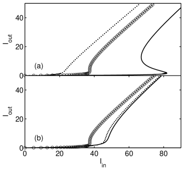
Figure 2: Examples of the input-output characteristics, demonstrating the occurrence of three-valued solutions to Eq. (12). In simulations, chains of $N=500$ sites and a disorder strength $\sigma=0.1J$ were used, corresponding to a HWHM $\sigma^{*}=0.0156J$. (a) - The results obtained for different superradiant constants $\Gamma_{R}$ at the optimal detuning $\Delta_{0}^{\mathrm{opt}}=-2.42J$, which corresponds to an incoming field which is resonant with the absorption maximum. The open circles, dotted, and solid curves represent, respectively, the data calculated for $\Gamma_{R}=16.61\sigma^{*}$ (the bistability threshold for $\sigma=0.1J$), $\Gamma_{R}=11.52\sigma^{*}$ (below the bistability threshold), and $27.12\sigma^{*}$ (above the bistability threshold). (b) - The results obtained for $\Gamma_{R}=16.61\sigma^{*}$ and various detunings $\Delta_{0}$. The dotted and solid curves represent, respectively, the data calculated for $\Delta_{0}=\Delta_{0}^{\mathrm{opt}}-\sigma^{*}$, and $\Delta_{0}^{\mathrm{opt}}+\sigma^{*}$. The open circles show the same data as in panel (a).

Several examples of the $S$-shaped input-output characteristics calculated for the disorder degree $\sigma=0.1J$ are shown in Fig. 2 for an input field that is resonant with the absorption maximum. We use the dimensionless intensities $I_{\mathrm{in}}=|\Omega_{i}|^{2}/(\gamma_{0}\sigma^{*})$ and $I_{\mathrm{out}}=|\Omega|^{2}/(\gamma_{0}\sigma^{*})$, which is convenient because the HWHM of the absorption spectrum $\sigma^{*}$ is an experimentally measurable quantity. Panel (a) shows how the input-output characteristics change when $\Gamma_{R}$ is below, at, or above its critical value. Panel (b) shows the input-output characteristics when the field is tuned through the resonance.

Figure 3: (a) - Dependence of the critical superradiant constant $\Gamma_{R}^{c}$ on the detuning $\Delta_{0}$ (solid line) calculated for the disorder strength $\sigma=0.1J$. The dashed line shows the absorption spectrum (absorption only due to $s$-states). The dotted horizontal line indicates $\Gamma_{R}^{c}$ calculated for the optimal detuning $\Delta^{\mathrm{opt}}_{0}=-2.42J$. (b) - Dependence of the switching intensity $I_{\mathrm{in}}^{c}$ on the detuning $\Delta_{0}$ calculated at the corresponding bistability threshold, i.e., with $\Gamma_{R}^{c}$ given in the panel (a).

At a given disorder strength $\sigma$, the minimal value of the superradiant constant $\Gamma_{R}$ needed for optical bistability (the critical value $\Gamma_{R}^{c}$) depends on the detuning $\Delta_{0}$. Figure 3(a) explicitly demonstrates this effect: $\Gamma_{R}^{c}$ is almost constant within the absorption band, whereas it clearly increases outside it. Panel (b) shows the $\Delta_{0}$-dependence of the critical switching intensity $I_{\mathrm{in}}^{c}$ of the incoming field at the bistability threshold. This is the lowest intensity at which the film can switch, when the field is tuned at $\Delta_{0}$, and when the superradiance constant $\Gamma_{R}=\Gamma_{R}^{c}(\Delta_{0})$. The data presented here is obtained for the disorder strength $\sigma=0.1J$.

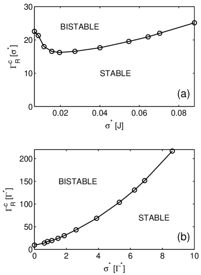
Figure 4: (a) - Phase diagram of the bistable optical response of a thin film in the $(\Gamma_{R},\sigma^{*})$-space obtained by solving Eq. (12) for $\Delta=\Delta_{0}^{\mathrm{opt}}$. The open circles represent the numerical data points, whereas the solid line is a guide to the eye. Above (below) the solid line the film behaves in a bistable (stable) fashion. The solid line itself represents the $\sigma^{*}$-dependence of the critical superradiant constant $\Gamma_{R}^{c}$, calculated for the optimal detuning $\Delta_{0}^{\mathrm{opt}}$, i.e., when the incoming field is tuned to the absorption band maximum. This gives the minimal $\Gamma_{R}^{c}$ for each $\sigma^{*}$. (b) - The same data points as in the panel (a), only replotted as a function of $\Gamma^{*}$, where $\Gamma^{*}$ is the mean value of the relaxation constant $\Gamma$.

As is seen from Fig. 3(a), there exists a detuning $\Delta_{0}^{\mathrm{opt}}$, referred to as the optimal one, at which $\Gamma_{R}^{c}$ takes its minimal value. The detuning is optimal if the imaginary term in Eq. (12) vanishes: this term opposes a three-valued solution for the output field. For a symmetric absorption band, the optimal detuning corresponds to the incoming field being resonant with the absorption maximum. In our case, owing to a small asymmetry of the absorption band [see Fig. 1(b)], $\Delta_{0}^{\mathrm{opt}}=-2.42J$ is shifted slightly to the blue from the position of the absorption peak.

We calculated $\Gamma_{R}^{c}$ as a function of the HWHM $\sigma^{*}$ for the optimal detuning. The result is shown in Fig. 4. The plot represents, in fact, the phase diagram of the optical response: below the curve, the output-input characteristic of the film is always single-valued (stable), while - depending on the detuning - it can become three-valued (bistable) above it. The nonmonotonic behavior of $\Gamma_{R}^{c}$ at small magnitudes of $\sigma^{*}$, presented in the panel a, is simply explained by the fact that the disorder-induced (inhomogeneous) broadening becomes smaller than the homogeneous one $\sigma^{*}<\Gamma^{*}$, where $\Gamma^{*}$ is defined as $\Gamma^{*}=\int d\mu d\varepsilon\,\Gamma{\cal G}_{s}(\varepsilon,\mu)$. The ratio $\Gamma_{R}/\Gamma^{*}$ is now the relevant parameter, governing the occurrence of bistability. The panel (b) shows the $\sigma^{*}$-dependence of $\Gamma_{R}^{c}$ replotted in units of $\Gamma^{*}$, which is monotonic. When $\sigma\to 0$, the ratio $\Gamma_{R}^{c}/\Gamma^{*}\to 9.64$. This value is deduced from Eq. (12). Indeed, in the limit of $\sigma\to 0$ we can move the Lorenztian outside the integral and use $\int d\Delta d\mu\,\mu^{2}{\mathcal{G}}_{s}(\Delta,\mu)=F_{s}/N_{s}$. The resulting equation is the same as for a thin film of homogeneously broadened two-level systems, only with the renormalized cooperative number ${\tilde{\Gamma}}_{R}/\Gamma^{*}=(\Gamma_{R}/\Gamma^{*})(F_{s}/N)$, where $F_{s}/N=0.83$. Bearing in mind that the critical value of the ratio ${\tilde{\Gamma}}_{R}/\Gamma^{*}$ is equal to 8, Zakharov88 we recover $\Gamma_{R}^{c}/\Gamma^{*}=9.64$.

IV.3 Spectral distribution of the exciton population

More insight into what occurs at the switching threshold is obtained by studying the population distribution

$$r_{11}(\Delta)=\int d\mu{\cal G}_{s}(\Delta,\mu)\rho_{11}(\Delta,\mu)\ ,$$ (13)

with $\rho_{11}$ the steady-state solution of Eqs. (6). This distribution enables us to visualize the relevant spectral range around the switching point.

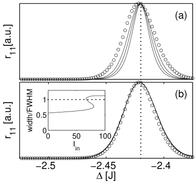
Figure 5: Population-distributions $r_{11}(\Delta)$ (solid curves), calculated according to Eq. (13) for $\sigma=0.1J$ and $\Gamma_{R}=27.12\sigma^{*}$, with the optimal detuning $\Delta_{0}^{\mathrm{opt}}=-2.42J$ indicated by the vertical dashed line. Open circles show the absorption spectrum $\mathcal{A}_{s}(\Delta)$. Panel (a) represents $r_{11}(\Delta)$ below the upper switching threshold. The plotted distributions were calculated for the input intensities $I_{\mathrm{in}}=|\Omega_{i}|^{2}/(\gamma_{0}\sigma^{*})=3.33,64.34$, and $81.78$ (from bottom to top). Panel (b) shows $r_{11}(\Delta)$ above the upper switching threshold. In the inset, the dependence of the full width at half maximum (FWHM) of $r_{11}(\Delta)$ on $I_{\mathrm{in}}$ is plotted in units of the FWHM of the absorption spectrum.

In Fig. 5, we plotted $r_{11}(\Delta)$ calculated for the optimal detuning $\Delta_{0}^{\mathrm{opt}}$ and $\Gamma_{R}=27.12\sigma^{*}$ (above the critical value $\Gamma_{R}^{c}$). Panels (a) and (b) show the results obtained for the incoming field intensities $I_{\mathrm{in}}=\Omega_{i}^{2}/(\gamma_{0}\sigma^{*})$ below and above the switching threshold, respectively. Below the switching threshold, only a relatively narrow spectral region around $\Delta^{\mathrm{opt}}_{0}$ acquires population. This is because, in spite of the intensities of the incoming field $I_{\mathrm{in}}=3.33,64.34$, and $81.78$ being far above the saturation value, the intensity of the field inside the film, $I_{\mathrm{out}}=\Omega_{i}^{2}/(\gamma_{0}\sigma^{*})$ $=0.025$, $0.5$, and $1.5$, is below or on the order of it. For these intensities, the one-exciton approximation, with only one $s$-like excited state considered in each localization segment, is reasonable.

Figure 5(b) represents the population distribution $r_{11}(\Delta)$ after switching, when the field inside the film $I_{\mathrm{out}}$ exceeds the switching threshold and becomes much larger than the saturation magnitude. In this limit, we can replace $\rho_{11}(\Delta,\mu)$ in Eq. (13) by 0.5 and get $r_{11}(\Delta)=0.5\int d\mu{\cal G}_{s}(\Delta,\mu)=0.5{\cal D}_{s}(\Delta)$, where ${\cal D}_{s}(\Delta)$ is the density of $s$-like states. The latter is plotted in Fig. 5 (b) by the solid line and appears to be wider than the absorption band. For such field intensities, it is likely that the two-level model should be corrected by including the one-to-two exciton transitions. This work is now in progress.

V Time-domain analysis

V.1 Hysteresis loop

It is well known that the S-shaped output-input dependence and, as a consequence, the existence of two switching thresholds results in optical hysteresis. Lugiato84 ; Gibbs85 To investigate this, we numerically integrated Eqs. (6) while slowly sweeping up-and-down the input intensity $I_{\mathrm{in}}$ above the bistability threshold ($\Gamma_{R}>\Gamma_{R}^{c}$). The result for the transmitted intensity $I_{\mathrm{out}}$ is shown in Fig. 6 by the solid curve with arrows. The parameters used in the calculations are specified in the figure caption. The input field intensity was swept from zero to 110 and back to zero. The open circles indicate the steady-state solution obtained by solving Eq. (12) for the same set of parameters.

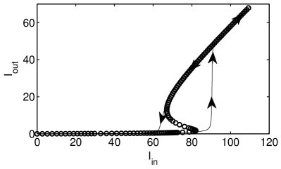
Figure 6: An example of the stable optical hysteresis loop of the transmitted intensity $I_{\mathrm{out}}=|\Omega|^{2}/(\gamma_{0}\sigma^{*})$ (the solid curve with arrows) obtained by numerically solving Eqs. (6) for a linear sweeping up-and-down of the input field intensity $I_{\mathrm{in}}=|\Omega_{i}|^{2}/(\gamma_{0}\sigma^{*})$. The sweeping time is $3000/\sigma^{*}$. The open circles represent the steady-state solution, Eq. (12). The calculations were performed for the following set of parameters: $\Gamma_{2}=500\gamma_{0}$, $\sigma=0.1J$, $\Gamma_{R}=27.12\sigma^{*}$, and $\Delta_{0}=\Delta_{0}^{\mathrm{opt}}=-2.42J$.

As can be seen from Fig. 6, the solid curve almost perfectly follows the lower and upper branches of the steady-state three-valued solution, nicely demonstrating the optical hysteresis. The intermediate branch is not revealed, which is clear evidence of its instability. Note also that switching from the lower branch to the upper one occurs for an input field intensity larger than the critical value. This indicates that when the input field intensity is only slightly above the switching intensity, the response of the film slows down. A much less pronounced but similar effect can be observed at the lower switching threshold, where the field switches from the upper branch to the lower one. This is consistent with our study of the relaxation time presented below.

V.2 Switching time

Of great importance from a practical point of view, is the relaxation time $\tau$ which is required for the output intensity to approach its steady-state value after the input intensity has changed. If this time is much shorter than the characteristic time of changing the input intensity, then the output signal will adiabatically follow it, remaining all the time close to the steady-state level. Only in the limit of short $\tau$, an abrupt switching from low to high transmittivity can be realized. This especially concerns the region in the vicinity of the switching thresholds (see Fig. 6). In other words, the relaxation time $\tau$ limits the usage of the optical bistable element as an instantaneous switcher.

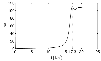
Figure 7: Kinetics of the transmitted field intensity $I_{\mathrm{out}}=|\Omega|^{2}/(\gamma_{0}\sigma^{*})$ approaching its stationary value (dashed line) after the incident field with intensity $I_{\mathrm{in}}=|\Omega_{i}|^{2}/(\gamma_{0}\sigma^{*})=150$ is turned on abruptly at $t=0$. The value $I_{\mathrm{in}}=150$ exceeds the upper switching threshold $I_{\mathrm{in}}^{c}=82.16$. The other parameters were chosen as in Fig. 6.

Motivated by the above observations, we performed a study of the relaxation time $\tau$. Figure 7 shows an example of how the transmitted field intensity approaches its stationary value when an input field intensity with a value of $I_{\mathrm{in}}=150$ is instantaneously switched on at $t=0$. This field is above the upper switching threshold $I_{\mathrm{in}}^{c}=82.16$. Calculations were carried out for the set of parameters of Fig. 6. As is observed, for the set of parameters used, the output intensity stays low during a waiting time of about $20/\sigma^{*}$, before it rapidly (on a time scale much shorter than $20/\sigma^{*}$) increases to its steady state value. This behavior allows one to define $\tau$ as the time which the output intensity takes to reach its first peak ($17.3/\sigma^{*}$ in the current example).

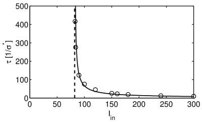
Figure 8: Relaxation time $\tau$ as a function of the excess input intensity $I_{\mathrm{in}}-I_{\mathrm{in}}^{c}$ at the upper switching threshold (indicated by the vertical dotted line). $\tau$ was calculated by turning on abruptly the incoming field at $t=0$, and waiting until the transmitted field intensity $I_{\mathrm{out}}$ approaches its steady-state value (for more details, see the text). The open circles show the numerical results, while the solid line represents a best power-law fit given by Eq. 14. The calculations were performed for the set of parameters of Fig. 6.

Using the above definition, we calculated the relaxation time $\tau$ as a function of the excess input intensity $I_{\mathrm{in}}-I_{\mathrm{in}}^{c}$ at the upper switching threshold. The results are plotted in Fig. 8. As is seen, $\tau$ drastically increases when $I_{\mathrm{in}}$ gets closer to $I_{\mathrm{in}}^{c}$. The numerical data (open circles) is well fitted by the formula

$$\tau=870\left(I_{\mathrm{in}}-I_{\mathrm{in}}^{c}\right)^{-0.83}\ ,$$ (14)

shown by the solid curve.

VI Discussion of driving parameters

To get insight into the possibility to realize optical bistable behavior for a film of J-aggregates, we consider the typical parameters for this type of systems. First, we estimate the superradiant constant $\Gamma_{R}=(3/8\pi)\gamma_{0}n_{0}\lambda^{2}L$, considering the low-temperature experimental data of J-aggregates of polymethine dyes. For these species, typically, $\gamma_{0}\approx(1/3)$ ns^-1 and $\lambda\approx 600$ nm. deBoer90 ; Fidder90 ; Minoshima94 ; Moll95 ; Kamalov96 ; Scheblykin00 With this in mind and choosing $L=\lambda/2\pi$  (or $kL=1$),we obtain the following estimate: $\Gamma_{R}\approx 10^{-18}n_{0}$ cm³ ps^-1. This value for $L$ is easily accessible with the spin-coating method Misawa93 and guarantees the applicability of the mean-field approach for the description of the thin film optical response. Jarque01 The typical width of the J-band of polymethine dyes is on the order of several tens of cm^-1 or approximately 1 ps^-1 (in frequency units). deBoer90 ; Fidder90 ; Minoshima94 ; Moll95 ; Kamalov96 ; Scheblykin00 Thus, for the set of parameters we chose, the number density of molecules $n_{0}$ must be on the order of $10^{19}$ cm^-3 to get the ratio $\Gamma_{R}/\sigma^{*}$ required for bistability to occur. This concentration is usually achieved in spin-coated films.

Another option to adjust the parameters favoring bistability is to consider $J$-aggregates composed of monomers with higher radiative constant $\gamma_{0}$ and a larger emission wavelength $\lambda$. From this point of view, J-aggregates of squarylium dyes may be suitable candidates. Furuki01 ; Tatsuura01 ; Pu02 This type of aggregates, spin-coated on a substrate, shows a sharp absorption peak at $\lambda\approx 800$ nm with HWHM = 20 nm at room temperature and a fast ($\sim 100$ fs) optical response Furuki01 ; Pu02 combined with a giant cubic succeptibility, Tatsuura01 both attributed to the excitonic nature of the optical excitations. The monomer decay time has been reported to be $\sim 100$ ps, Furuki01 ), although no information about the quantum yield has been presented. If we assume that this time is of radiative nature, the superradiant constant $\Gamma_{R}$ can be adjusted to values above the bistability threshold even for smaller concentration of monomers in the film. On the other hand, for larger $\gamma_{0}$ also the intensity required for switching increases, which is not desired because of the limited photostability of most J-aggregates.

VII Summary and concluding remarks

We theoretically studied the optical response of an ultrathin film of oriented J-aggregates, with the goal to examine the possibility of bistable behavior of the system. The standard Frenkel exciton model was used for a single aggregate: an open linear chain of monomers coupled by delocalizing dipole-dipole excitation transfer interactions, in combination with uncorrelated on-site disorder, which tends to localize the exciton states. We considered a single aggregate as a meso-ensemble of two-level systems, each one composed of an $s$-like localized one-exciton state and its own ground state. The one-to-two exciton transitions have been neglected.

As a tool to describe the transmission properties of the film, we employed the optical Maxwell-Bloch equations adapted for a thin film. The electric polarization of the film was calculated by making use of a joint probability distribution of exciton energies and transition dipole moments, properly taking into account the correlation properties of these two stochastic variables. The joint distribution function was calculated by numerically diagonalizing the Frenkel Hamiltonian and averaging over many disorder realizations.

We derived a novel steady-state equation for the transmitted signal in terms of the joint distribution function, and demonstrated that three-valued solutions to this equation exist in a certain domain of the parameter space $(\Gamma_{R},\sigma^{*})$,where $\Gamma_{R}$ is the superradiant constant and $\sigma^{*}$ is the half-width-at-half-maximum of the absorption band. Our approach allowed us to generalize previous results Malyshev00 ; Jarque01 to correctly account for the stochastic nature of the exciton energy and transition dipole moment. Using the new steady-state equation, we have found that the critical value of the so-called ”cooperative number” $\Gamma_{R}/\sigma^{*}$, Lugiato84 which governs the occurrence of bistability of the film, is higher than obtained before. Malyshev00 Moreover, in contrast to Refs. Malyshev00, and Jarque01, , we have analyzed the switching time, which show a dramatic increase for input intensities close to the switching point. We also found that the ”cooperative number” $\Gamma_{R}/\sigma^{*}$ increases with $\sigma^{*}$, but only slightly, varying between 12 and approximately 25 within a wide range of $\sigma^{*}$. Estimating the parameters of our model for aggregate of polymethin dyes shows that these are a promising candidate to measure the effect.

Finally, we note that also the microcavity arrangement of molecular aggregates Lidzey98 ; Litinskaya04 ; Beltyugov04 ; Agranovich05 ; Zoubi05 is of interest for applications. During the last decade, organic microcavities have received a great deal of attention because of the strong coupling of the excitons to cavity photons, leading to giant polariton splitting in these devices. Lidzey03 The recent observation of optical bistability in planar inorganic microcavities Baas04 in the strong coupling regime suggests that organic microvavities can exhibit a similar behavior.

Appendix A Estimates of quantum interference effects

Our approach to the optical dynamics of a single aggregate was based on the representation of the aggregate as a meso-ensemble of two-level systems with their own ground states. The model has its origin in the fact that the optically dominant exciton states are localized on different segments and overlap weakly. In reality, however, the ground state of an aggregate (all the monomers are in their ground states) is common for all (multi- ) exciton states. This results in cross-interference of field-induced as well as spontaneous transitions. Below, we provide estimates of these additional terms and show that in the limit of dominant inhomogeneous broadening of the J-band, the cross-interference effects can be neglected. In our estimates, we will only consider ground state-to-one-exciton transitions.

We start with the equation for the density operator $\rho$

$$\dot{\rho}=-\frac{i}{\hbar}\left[H_{0}-{\hat{d}}\mathcal{E},\rho\right]-R^{\mathrm{bath}}\rho-R^{\mathrm{rad}}\rho\ ,$$ (15)

where $H_{0}$ is the exciton Hamiltonian specified in Eq. (1) and the term $-{\hat{d}}\mathcal{E}$ describes the interaction of the aggregate with the field $\mathcal{E}$ inside the film. $R^{\mathrm{bath}}$ represents the dephasing operator, acting as follows:

$$\langle\nu|R^{\mathrm{bath}}\rho\,|\nu^{\prime}\rangle = (1-\delta_{\nu\nu^{\prime}})(\gamma_{\nu 0}+\gamma_{\nu^{\prime}0})\rho_{\nu\nu^{\prime}}\ ,$$

$$\langle\nu|R^{\mathrm{bath}}\rho\,|0\rangle = \gamma_{\nu 0}\rho_{\nu 0}\ .$$ (16)

Here, $\gamma_{\nu 0}$ is the (pure) dephasing rate of the exciton transition $|\nu\rangle\to|0\rangle$, excluding radiative decay. These constants will be considered on a phenomenological basis.

The operator $R^{\mathrm{rad}}$ governs the exciton radiative relaxation. It is given by (see, e.g., Ref. Blum96, )

$$R^{\mathrm{rad}}\rho = \frac{1}{2}\>\sum_{\nu\nu^{\prime}}\gamma_{\nu\nu^{\prime}}\Big{[}\,|\nu\rangle\langle\nu^{\prime}|\,\rho$$ (17)

$$+ \rho\,|\nu\rangle\langle\nu^{\prime}|-2\,|0\rangle\langle\nu|\,\rho\,|\nu^{\prime}\rangle\langle 0|\>\Big{]}\ ,$$

where $\gamma_{\nu\nu}=\gamma_{0}\big{(}\sum_{n}\varphi_{\nu n}\big{)}^{2}$ is the radiative decay rate of the population of the $\nu$th state. Furthermore, $\gamma_{\nu\nu^{\prime}}=\gamma_{\nu^{\prime}\nu}$   ($\nu\neq\nu^{\prime}$) describes the quantum interference in the radiative relaxation of the $\nu$th and $\nu^{\prime}$th states, resulting from the cross-coupling of different decay channels. It reflects the fact that a state $\nu$, when decaying, drives another state $\nu^{\prime}$ and vice versa. If the transition dipoles of all the states are parallel, $\gamma_{\nu\nu^{\prime}}=(\gamma_{\nu\nu}\gamma_{\nu^{\prime}\nu^{\prime}})^{1/2}$.

Using Eqs. (A) and (17) in Eq. (15), we arrive at the following set of equations for the density matrix elements:

$$\dot{\rho}_{\nu\nu}=-\gamma_{\nu\nu}\rho_{\nu\nu}-\frac{1}{2}\sum_{\nu^{\prime}\neq\nu}\gamma_{\nu\nu^{\prime}}\left(\rho_{\nu\nu^{\prime}}+\rho_{\nu^{\prime}\nu}\right)+id_{\nu}\mathcal{E}\left(\rho_{\nu 0}^{*}-\rho_{\nu 0}\right)\ ,$$ (18a)

$$\dot{\rho}_{\nu\nu^{\prime}}=-(i\varepsilon_{\nu\nu^{\prime}}+\Gamma_{\nu\nu^{\prime}})\rho_{\nu\nu^{\prime}}-\frac{1}{2}\sum_{\nu^{\prime\prime}\neq\nu}\gamma_{\nu\nu^{\prime\prime}}\rho_{\nu^{\prime\prime}\nu^{\prime}}-\frac{1}{2}\sum_{\nu^{\prime\prime}\neq\nu^{\prime}}\gamma_{\nu^{\prime\prime}\nu^{\prime}}\rho_{\nu\nu^{\prime\prime}}+i\left(d_{\nu}\mathcal{E}\rho_{\nu^{\prime}0}^{*}-\rho_{\nu 0}d_{\nu^{\prime}}\mathcal{E}\right)\ ,\quad\quad\nu\neq\nu^{\prime}\ ,$$ (18b)

$$\dot{\rho}_{\nu 0}=-(i\varepsilon_{\nu}+\Gamma_{\nu 0})\rho_{\nu 0}-\frac{1}{2}\sum_{\nu^{\prime}\neq\nu}\gamma_{\nu\nu^{\prime}}\rho_{\nu^{\prime}0}-i\sum_{\nu^{\prime}\neq\nu}\rho_{\nu\nu^{\prime}}d_{\nu^{\prime}}\mathcal{E}-id_{\nu}\mathcal{E}\left(\rho_{\nu\nu}-\rho_{00}\right)\ ,$$ (18c)

$$\rho_{00}+\sum_{\nu}\rho_{\nu\nu}=1\ .$$ (18d)

Here we introduced the notations: $\varepsilon_{\nu\nu^{\prime}}=\varepsilon_{\nu}-\varepsilon_{\nu^{\prime}}$, $\Gamma_{\nu\nu^{\prime}}=\frac{1}{2}(\gamma_{\nu\nu}+\gamma_{\nu^{\prime}\nu^{\prime}})+\gamma_{\nu 0}+\gamma_{\nu^{\prime}0}$, and $\Gamma_{\nu 0}=\frac{1}{2}\gamma_{\nu\nu}+\gamma_{\nu 0}$.

Equations (18) differ from those used in the two-level model, Eq. (2), by several terms. Because all the exciton states have the same ground state, which is reflected in the normalization condition (18d), the low-frequency coherences are now involved in the aggregate optical dynamics. They are coupled to the populations [Eq. (18a)] as well as to the high-frequency (optical) coherences $\rho_{\nu 0}$ [Eqs. (18b) and (18c)] via both the cross-coupling of the transitions and the field. In addition, the cross-coupling also couples the optical coherences $\rho_{\nu 0}$ [Eq. (18c)].

In quantum optics of atomic gases, the cross-coupling of transitions has been found to be the origin of many fascinating effects, such as narrow resonances, transparency and gain without population inversion (see for an overview Refs. Kocharovskaya92, ; Arimondo96, ; Harris97, ; Fleischhauer05, ), as well as bistability at a low threshold. Walls80 ; Anton02 ; Joshi04 All these effects, however, require specific conditions: equivalent magnitudes of all the $\gamma_{\nu\nu}$ and the absence of dephasing and inhomogeneous broadening. Any deviation from these requirements washes out those effects. In particular, this happens for J-aggregates; below we argue why all the cross-terms in Eqs. (18) can be neglected for these systems.

The contribution of the cross-terms to a given state $\nu$ always comes in the form of a summation over all other states $\nu^{\prime}$. The optical dynamics of the system is determined by only several dominant states. If $N^{*}$ is the typical localization length, there will be $N/N^{*}$ of such states. They are spread over the width of the absorption band, given by $2\sigma^{*}$. Therefore we can estimate the sum under consideration by $(\gamma^{*}/2\sigma^{*})(N/N^{*})\sim\gamma_{0}N/2\sigma^{*}$, where $\gamma^{*}=\gamma_{0}N^{*}$ is the typical radiative rate of optically dominant states. The materials we consider typically have $\gamma_{0}\sim 10^{8}$ s${}^{-1}\sim 10^{-2}$ cm^-1 and $2\sigma^{*}$ on the order of several tens of cm^-1. Then, for an aggregate of length $N=500$ the ratio $\gamma_{0}N/2\sigma^{*}\sim 0.1$. On this basis, we neglect all the cross-coupling terms in Eqs. (18) and replace the normalization condition (18d) for the whole aggregate by the one for a single segment, $\rho_{00}+\rho_{\nu\nu}=1$.

References

- (1) L. F. Mollenauer, R. H. Stolen, and J. P. Gordon, Phys. Rev. Lett. 45, 1095 (1980).
- (2) A. Hasegava and J. Kodamam, Solitons in Opical Commuications (Oxford University Press, Oxford, 1995).
- (3) P. St. J. Russell, Science 299, 358 (2003).
- (4) O. Wada, New J. Phys. 6, 183 (2004).
- (5) V. R. Almeida, C. A. Barrios, R. R. Panepucci, and M. Lipson, Nature 431, 1081 (2004).
- (6) A. M. C. Dawes, L. Illing, S. M. Clark, D. J. Gauthier, Science 308, 672 (2004).
- (7) S. L. McCall, Phys. Rev. A 9, 1515 (1974).
- (8) H. M. Gibbs, S. L. McCall, and T. N. C. Venkatesan, Phys. Rev. Lett. 36, 1135 (1976).
- (9) E. Abraham and S. D. Smith, Rep. Prog. Phys., 45, 815 (1982).
- (10) L. A. Lugiato, in Progress in Optics, ed. E. Wolf (North-Holland, Amsterdam, 1984), vol. XXI, p. 71.
- (11) H. M. Gibbs, Optical Bistability: Controlling Light with Light (Academic, New York, 1985).
- (12) N. N. Rosanov, in Progress in Optics, ed. E. Wolf (North-Holland, Amsterdam, 1996), vol. XXXV, p. 1.
- (13) M. P. Hehlen, H. U. Güdel, Q. Shu, J. Rai, S. Rai, and S. C. Rand, Phys. Rev. Lett. 73, 1103 (1994). M. P. Hehlen, H. U. Güdel, Q. Shu, and S. C. Rand, J. Chem. Phys. 104, 1232 (1996). M. P. Hehlen, A. Kuditcher, S. C. Rand, and S. R. Lüthi, Phys. Rev. Lett. 82, 3050 (1999).
- (14) N. Bodenschatz and J. Heber, Phys. Rev. A 54, 4428 (1996); J. Alloys Compd. 300-301, 32 (2000).
- (15) O. Guillot-Noël, L. Binet, and D. Gourier, Chem. Phys. Lett. 344, 612 (2001); Phys. Rev. B 65, 245101 (2002); O. Guillot-Noël, Ph. Goldner, and D. Gourier, Phys. Rev. A 66, 063813 (2002).
- (16) V. A. Malyshev, H. Glaeske, and K.-H. Feller, Phys. Rev. A 58, 1496 (1998).
- (17) F. Cicarello, A. Napoli, A. Mesina, and S. R. L üthi, Chem Phys. Lett. 381, 163 (2003); J. Opt. B: Quantum Semoclass. Opt. 6, 5118 (2004).
- (18) D. R. Gamelin, S. R. Lüthi, and H. U. Güdel, J. Phys. Chem. B 104, 11045 (2000).
- (19) M. A. Noginov, M. Vondrova, and B. D. Lucas, Phys. Rev. B 65, 035112 (2001). M. A. Noginov, M. Vondrova, and D. Casimir, Phys. Rev. B 68, 195119 (2003).
- (20) Ph. Goldner, O. Guillot-Noël, and P. Higel, Opt. Mater. 26, 281 (2004).
- (21) B. I. Greenham, S. C. Moratti, D. D. C. Bradly, R. H. Friend, and A. B. Holmes, Nature 365, 628 (1993).
- (22) G. Kranzelbinder and G. Leising, Rep. Prog. Phys. 63, 729 (2000).
- (23) F. C. Spano and J. Knoester, Adv. Magn. Opt. Res. 18, 117 (1994).
- (24) See the contributions to J-aggregates, edited by T. Kobayashi (World Scientific, Singapore, 1996).
- (25) See the contributions to ”Semiconducting Polymers - Chemistry, Physics, and Engineering”, eds. G. Hadziioannou and P. van Hutten (VCH, Weinheim, 1999).
- (26) H. van Amerongen, L. Valkunas, R. van Grondelle, Photosynthetic Excitons (World Scientific, Singapore, 2000).
- (27) J. Knoester, in Proceedings of the International School of Physics ”Enrico Fermi”, Course CXLIX, edited by V. M. Agranovich and G. C. La Rocca (IOS Press, Amsterdam, 2002), p. 149.
- (28) F. C. Spano, Annu. Rev. Phys. Chem. 57, 217 (2006).
- (29) G. D. Scholes and G. Rumbles, Nature Mater. 5, 683 (2006).
- (30) V. A. Malyshev and P. Moreno, Phys. Rev. A 53, 416 (1996); V. A. Malyshev, H. Glaeske and K.-H. Feller, Opt. Commun. 140, 83 (1997); Phys. Rev. A 58, 670 (1998).
- (31) V. A. Malyshev, H. Glaeske, and K.-H. Feller, Opt. Commun. 169, 177 (1999); J. Chem. Phys. 113, 1170 (2000).
- (32) V. A. Malyshev and E. Conejero-Jarque, Opt. Express 6, 227 (2000); E. Conejero-Jarque and V. A. Malyshev, J. Chem. Phys. 115 4275 (2001).
- (33) H. Glaeske, V. A. Malyshev, and K.-H. Feller, J. Chem. Phys. 114 1966 (2001); Phys. Rev. A 114, 033821 (2002).
- (34) D. B. Chesnut and A. Suna, J. Chem. Phys. 39, 146 (1963).
- (35) V. M. Agranovich, Theory of Excitons (Moscow, Nauka, 1968), in Russian.
- (36) F. C. Spano, Phys. Rev. Lett. 67, 3424 (1991).
- (37) S. M. Zakharov and E. A. Manykin, Poverkhnost’ 2, 137 (1988); A. M. Basharov, Zh. Exp. Teor. Fiz. 94, 12 (1988) [JETP 67, 1741 (1988)]; A. N. Oraevsky, D. J. Jons, and D. K. Bandy, Opt. Commun. 111, 163 (1994).
- (38) V. Malyshev and P. Moreno, Phys. Rev. B 51 14587 (1995).
- (39) A. V. Malyshev and V. A. Malyshev, Phys. Rev. B 63 195111 (2001); J. Lumin. 94-95, 369 (2001).
- (40) I. M. Lifshits, Zh. Experim. Theor. Fiz. 53, 743 (1968) [Sov. Phys. JETP 26, 462 (1968)].
- (41) M. Bednarz, V. A. Malyshev, and J. Knoester, J. Chem. Phys. 120, 3827 (2004).
- (42) K. Misawa, K. Minoshima, H. Ono, and T. Kobayashi, Appl. Phys. Lett. 63, 577 (1993).
- (43) D. J. Heijs, V. A. Malyshev, and J. Knoester, Phys. Rev. Lett. 95, 177402 (2005); J. Chem. Phys. 123, 144507 (2005).
- (44) M. G. Benedict and E. D. Trifonov, Phys. Rev. A 38, 2854 (1988); M. G. Benedict, V. A. Malyshev, E. D. Trifonov, and A. I. Zaitsev, Phys. Rev. A 43, 3845 (1991).
- (45) M. G. Benedict, A. M. Ermolaev, V. A. Malyshev, I. V. Sokolov, and E. D. Trifonov, Super-radiance: Multiatomic coherent emission (Bristol and Philadelphia: Institut of Physics Publishing, 1996).
- (46) Y. C. Lee and P. S. Lee, Phys. Rev. B 10, 344 (1974).
- (47) S. de Boer and D.A. Wiersma, Chem. Phys. Lett. 165, 45 (1990).
- (48) H. Fidder, J. Knoester, and D.A. Wiersma, Chem. Phys. Lett. 171, 529 (1990).
- (49) K. Minoshima, M. Taiji, K. Misawa, T. Kobayashi, Chem. Phys. Lett. 218 67 (1994).
- (50) J. Moll, S. Daehne, J.R. Durrant, and D.A. Wiersma, J. Chem Phys. 102, 6362 (1995).
- (51) V.F. Kamalov, I.A. Struganova, and K. Yoshihara, J. Phys. Chem. 100, 8640 (1996).
- (52) I.G. Scheblykin, M.M. Bataiev, M. Van der Auweraer, A.G. Vitukhnovsky, Chem. Phys. Lett. 316, 37 (2000).
- (53) M. Furuki, M. Tian, Y. Sato, L. S. Pu, H. Kawashima, S. Tatsuura, and O. Wada, Appl. Phys. Lett. 78, 2634 (2001).
- (54) S. Tatsuura, O. Wada, M. Tian, M. Furuki, Y. Sato, I. Iwasa, L. S. Pu, and H. Kawashima, Appl. Phys. Lett. 79, 2517 (2001).
- (55) L. S. Pu, Opt. Mater. 21, 489 (2002).
- (56) D. G. Lidzey, D. D. C. Bradley, M. S. Skolnick, T. Virgili, S. Walker, and D. M. Whiteker, Nature 395, 53 (1998); D. G. Lidzey, D. D. C. Bradley, T. Virgili, A. Armitage, M. S. Skolnick, and S. Walker, Phys. Rev. Lett. 82, 3316 (1999).
- (57) M. Litinskaya, P. Reineker, and V. M. Agranovich, Phys. Stat. Sol. (a) 201, 646 (2004).
- (58) V. N. Bel’tyugov, A. I. Plekhanov, and V. V. Shelkovnikov, J. Opt. Technol. 71, 411 (2004).
- (59) V. M. Agranovich and G.C. La Rocca, Sol. St. Commun. 135, 544 (2005).
- (60) H. Zoubi and G. C. La Rocca, Phys. Rev. B 71, 235316 (2005).
- (61) D. G. Lidzey, in ”Thin Films and Nanostructures”, eds. V. M. Agranovich and F. Bassani (Elsevier, New York, 2003), Vol. 31, Chapt. 8.
- (62) A. Baas, J. Ph. Karr, H. Eleuch, and E. Giacobino, Phys. Rev. A 69, 023809 (2004).
- (63) K. Blum, The Density Matrix Theory and Applications, 2nd Edition (Plenum Press, New York and London, 1996).
- (64) O. A. Kocharovskaya, Phys. Rep. 219, 175 (1992).
- (65) E. Arimondo, in Progress in Optics, ed. E. Wolf (North-Holland, Amsterdam, 1996), vol. XXXV, p. 257.
- (66) S. E. Harris, Phys. Today 50, 36 (1997).
- (67) M. Fleischhauer, A. Imamoglu, and J. P. Marrangos, Rev. Mod. Phys. 77, 633 (2005).
- (68) D. F. Walls and P. Zoller, Opt. Commun. 34, 260 (1980); D. F. Walls, P. Zoller, and M. L. Steÿn-Ross, IEEE J. Quantum Electron. 17, 380 (1981).
- (69) M. A. Antón and O. G. Calderón, J. Opt. B 4, 91 (2002); M. A. Antón, O. G. Calderón, and F. Careño, Phys. Lett. A 311, 297 (2003).
- (70) A. Joshi, W. Yang, and M. Xiao, Phys. Rev. A 70, 041802(R) (2004).