Sine-Gordon description of Beresinskii-Kosterlitz-Thouless physics
at finite magnetic field

Abstract

The Beresinskii-Kosterlitz-Thouless (BKT) physics of vortices in two-dimensional superconductors at finite magnetic field is investigated by means of a field-theoretical approach based on the sine-Gordon model. This description leads to a straightforward definition of the field-induced magnetization and shows that the persistence of non-linear effects at low fields above the transition is a typical signature of the fast divergence of the correlation length within the BKT theory.

The Beresinskii-Kosterlitz-Thouless (BKT) transition Berezinsky (1972), namely the possibility to have a phase transition with a vanishing order parameter but algebraic decay of the correlations, is undoubtedly one of the most fascinating aspects of collective phenomena. It finds experimental realizations in a wide range of systems, as superfluids or superconducting (SC) filmsMinnaghen (1987); Crane et al. (2007); Matthey et al. (2006); Pourret et al. (2007) and recently cold atomic systems Hadzibabic et al. (2006). One of the key ingredients of the BKT transition is the existence of vortices, that unbind in the high-temperature phase leading to an exponential decay of the correlations. In order to treat such unbinding transition a very fruitful analogy was to represent the vortices as charges performing a Debye-Huckel screening transition in a neutral Coulomb-gas problem, for which a renormalization group procedure can be implemented Minnaghen (1987).

One specially interesting extension of the BKT transition is when a magnetic field is present, which will impose a population of vortices with a given vorticity in the system. This has found recent experimental application to thin filmsCrane et al. (2007); Pourret et al. (2007) or layered high-T_c superconductorsLi et al. (2005). Even in cold atomic systems, a magnetic field can be mimicked by imposing a rotation on the condensate Hadzibabic et al. (2006); Cazalilla et al. (2007). For all these systems it is thus crucial to predict theoretically how the magnetic field will affect the BKT transition and the various physical observables.

Due to the strong interest of such a question, this problem has been addressed in the past Minnaghen (1987); Doniach and Huberman (1979); Minnaghen (1981); V. Oganesyan and Sondhi (2006). Unfortunately, contrarily to the case of the ${\bf B}=0$ transition, the efforts have been partly unsatisfactory. In particular most of the literature on the subject rested on extending the mapping to the Coulomb-gas problem, where the effects of the magnetic field can be incorporated as an excess of positive charges. However this mapping gives the physical observables as a function of the magnetic induction ${\bf B}$ instead of the magnetic field ${\bf H}$, which is not convenient to describe the physics at low applied field.

An alternative approach to the BKT transition, which is of course well known for ${\bf B}=0$, is to use the mapping onto the sine-Gordon problemMinnaghen (1987); Giamarchi (2004), which was reviewed recently both in the context of quasi-2D superconductors Benfatto et al. (2007); Nandori (2007) and cold atomic systems Cazalilla et al. (2007). In this Letter we show that this description provides a very simple and physically transparent way to deal with the finite magnetic field case. In our scheme the physical observables have a straightforward definition, and the role of both ${\bf B}$ and ${\bf H}$ is clarified. In addition we also present a variational calculation of the field-induced diamagnetism in thin films. It leads to a detailed description of the Meissner phase below $T_{BKT}$ and of the appearance above $T_{BKT}$ of a non-linear magnetization at relatively low fields, in contrast to what expected from standard Ginzburg-Landau (GL) SC fluctuationsKoshelev (1994).

As a starting model we consider the $XY$ model for the phase of a 2D superconductorMinnaghen (1987)

$$H=J\sum_{<i,j>}[1-\cos(\theta_{i}-\theta_{j}-F_{ij})].$$ (1)

Here $\theta_{i,j}$ is the SC phase on two nearest-neighbor sites $(i,j)$ of a coarse-grained 2D lattice, $J={\Phi_{0}^{2}d}/16\pi^{3}\lambda^{2}$ is the 2D superfluid stiffness for a film of thickness $d$ and in-plane penetration depth $\lambda$, and we employed a minimal-coupling scheme for the vector potential ${\bf A}$, with $F_{ij}=(2\pi/\Phi_{0})\int_{i}^{j}{\bf A}\cdot d{\bf l}$, and $\Phi_{0}=hc/2e$ the flux quantum. Due to the periodicity of $H$ when $\theta\rightarrow\theta+2\pi$, beyond long-wavelength phase excitations where $\theta_{i}-\theta_{j}\approx a\nabla\theta$ varies smoothly on the lattice scale $a$, vortex configurations are allowed where $\oint\nabla\theta=\pm 2\pi$ over a closed loop. They emerge clearly by performing the standard dual mapping of the model (1)José et al. (1977). This allows us to write the partition function of the system as a functional integral over a scalar field $\phi$ as $Z=\int{\cal{D}}\phi e^{-S_{B}}$,

$$S_{B}\!=\negthickspace\!\int\!\!d{\bf r}dz\!\!\left[\frac{(\nabla\phi)^{2}}{2\pi K}\!-\!\frac{g}{\pi a^{2}}\cos 2\phi+\frac{2i}{\Phi_{0}}{\bf A}\!\cdot\!(\nabla\times\hat{z}\phi)\right]\!\delta(z),\,$$ (2)

where $\phi$ depends on the in-plane coordinates ${\bf r}$ only while ${\bf A}$ depends in general also on the $z$ coordinate. The $\delta(z)$ function gives the proper boundary conditions for a truly 2D case (where there is no SC current outside the plane). In the physical case of a SC film of thickness $d$ we assume that the sample quantities are averaged over $|z|<d/2$. In Eq. (2) we defined $K=\pi J/k_{B}T$ and $g=2\pi e^{-\beta\mu}$, where $\mu$ is the chemical potential of the vortices and $e^{-\beta\mu}$ their fugacity ($\beta=1/k_{B}T$). While in the $XY$ model $\mu/J$ is fixed, $\mu_{XY}\simeq\pi^{2}J/2$, we consider it as an independent variableBenfatto et al. (2007). In the dual representation (2) of the XY model (1) the cosine term accounts for vortex excitations: indeed, since $\phi$ is the dual field of $\theta$, a vortex, which is a $\pm 2\pi$ kink in the $\theta$ variable, is generated by the operator $e^{-\beta\mu}e^{\pm i2\phi}$. At high $T$ $\phi$ localizes in a minimun of the cosine and its conjugate field $\theta$ is completely disordered, i.e. the system looses the superfluid behavior. The interaction $V({\bf r})$ between vortices (or charges in the Coulomb-gas analogyMinnaghen (1987); Giamarchi (2004)) follows from the Gaussian part of the action (2), $V({\bf r})=\int d^{2}{\bf k}e^{i{\bf k}\cdot{\bf r}}V({\bf k})$ where $V({\bf k})=\langle|\phi({\bf k})|^{2}\rangle$, and it is logarithmic since $V({\bf k})=2\pi K/{\bf k}^{2}$.

The physical observables can be easily read out from Eq. (2) and the free energy $F=-k_{B}T\ln Z$. For example, the electric current is:

$${\bf J}_{s}({\bf r},z)=-c\frac{\partial F}{\partial{\bf A}({\bf r},z)}=-\frac{2ick_{B}T}{\Phi_{0}}\langle\nabla\times\hat{z}\phi({\bf r})\rangle\delta(z),$$ (3)

and it is purely transverse, as expected for vortex excitations. The magnetization ${\bf M}=({\bf B}-{\bf H})/4\pi$ is defined, as usual, as the functional derivative of $F$ with respect to ${\bf B}({\bf r},z)=\nabla\times{\bf A}$. By integrating by part, we can write the last term of Eq. (2) as $(2i/\Phi_{0})\int d{\bf r}dz\ [{\bf B}({\bf r},z)\cdot\hat{z}\phi({\bf r})]\delta(z)$, so that:

$${\bf M}({\bf r})=-\frac{1}{d}\int dz\frac{\partial F}{\partial{\bf B}({\bf r},z)}=-\hat{z}\frac{2ik_{B}T}{d\Phi_{0}}\left\langle\phi({\bf r})\right\rangle,$$ (4)

which leads to ${\bf J}_{s}=c(\nabla\times{\bf M})$Landau and Lifchitz (1984). Finally, by exploiting the fact that $e^{-\beta\mu}e^{\pm i2\phi}$ is the operator which creates up and down vortices with density $n_{\pm}$ respectively, we have a straightforward definition of the average vortex number $n_{F}=a^{2}(\langle n_{+}\rangle+\langle n_{-}\rangle)$ and of the excess vortex number $n=a^{2}(\langle n_{+}\rangle-\langle n_{-}\rangle)$ per unit cell as a function of $\phi$ as:

$$n_{F}=2e^{-\beta\mu}\langle\cos(2\phi)\rangle,\quad n=2e^{-\beta\mu}\langle\sin(2\phi)\rangle.$$ (5)

In Eq. (4) the average value of $\phi$ is computed with the action (2), so that it gives ${\bf M}$ as a function of the magnetic induction ${\bf B}$. To obtain ${\bf M}$ as a function of the applied field ${\bf H}$ we must use the Gibbs free energy ${\cal{G}}=-k_{B}T\ln Z$, where $Z=\int{\cal{D}}\phi{\cal{D}}Ae^{-S}$ and:

$$S=S_{B}+\int{d{\bf r}dz}\left\{\frac{(\nabla\times{\bf A})^{2}}{8\pi k_{B}T}-\frac{(\nabla\times{\bf A})\cdot{\bf H}}{4\pi k_{B}T}\right\}.$$

${\bf H}$ satisfies the Maxwell equation $\nabla\times{\bf H}=(4\pi/c){\bf J}_{ext}$ for a given distribution ${\bf J}_{ext}$ of external currents. By integrating out ${\bf A}$ in the radial gauge $\nabla\cdot{\bf A}=0$, the action reduces to:

$$S=\int\frac{d^{2}{\bf k}}{(2\pi)^{2}}\frac{k^{2}+k\Lambda^{-1}}{2\pi K}|\phi({\bf k})|^{2}-\frac{g}{\pi a^{2}}\int d{\bf r}\cos 2\phi,$$

$$+\frac{2i}{\Phi_{0}}\int d{\bf r}\,\phi\,\hat{z}\cdot{\bf H}^{0}({\bf r},z=0)-\int d{\bf r}dz\frac{({\bf H}^{0})^{2}}{8\pi k_{B}T},$$ (6)

where $1/\Lambda=d/2\lambda^{2}={8\pi^{2}Kk_{B}T}/{\Phi_{0}^{2}}$. Here ${\bf H}^{0}$ is the magnetic field generated by ${\bf J}_{ext}$ in the vacuum, i.e. it satisfies the same Maxwell equation as ${\bf H}$, but it is not constrained to the boundary condition that ${\bf B}=0$ in the SC film. Thus, using the Laplace formula ${\bf H}^{0}({\bf r})=(1/c)\int d^{3}{\bf r}^{\prime}[{\bf J}_{ext}({\bf r}^{\prime})\times({\bf r}-{\bf r}^{\prime})]/|{\bf r}-{\bf r}^{\prime}|^{3}$. The effect of integrating out the ${\bf B}$ field is twofold. First, one introduces an effective screening of the vortex potential $V({\bf r})$. Indeed, thanks to the $k\Lambda^{-1}$ term in Eq. (6), $V({\bf r})\sim\log(r/a)$ up to a scale of order $\Lambda$, and then decays as $\Lambda/r$Minnaghen (1987, 1981). Second, one couples directly the dual field $\phi$ to the reference field ${\bf H}^{0}$ used in the experiments. We thus expect that in the Meissner phase ${\bf M}$ includes automatically the demagnetization effects, i.e. $-4\pi{\bf M}={\bf H}^{0}/(1-\eta)$Landau and Lifchitz (1984), where $\eta$ is the demagnetization constant which depends only on the sample geometry and is near to 1 in a film, $\eta\sim 1-d/R$Landau and Lifchitz (1984); Fetter and Hohenberg (1967), where $R$ is the transverse film dimension.

The model (6) and the constitutive equations (3)-(5) establish a clear and general theoretical framework to address the physics of 2D SC films in a magnetic field. To illustrate their usefulness we solve them by using a variational approximation. The idea is to replace the cosine interaction in Eq. (6) with a mass term $\Delta^{2}\phi^{2}$, where $\Delta$ is determined self-consistently by minimizing the variational energy ${\cal{G}}_{var}={\cal{G}}_{0}+T\langle S-S_{0}\rangle$, $S_{0}$ being the trial action. At ${\bf H}^{0}=0$ a finite $\Delta$ appears above $T_{BKT}$, which signals the localization of $\phi$ in a minimum of the cosine, and cut-off at a scale $1/\Delta$ the logarithmic vortex potential $V({\bf r})$. This allows for the proliferation of free-vortex excitations. We then consider the case of a perpendicular field ${\bf H}=H\hat{z}$ (in the following we drop the superscript $0$) slowly varying over the film. To account for it we introduce in the trial action an additional variational parameter $\bar{H}$, coupled linearly to $\int d{\bf r}\phi$ in analogy with Eq. (6), so that only the $\phi(k)$ component at the minimum $k$ value $k_{min}\simeq 1/R$ couples to $H$. A finite system size $R$ is needed to have finite demagnetization in the Meissner phase, but its role at large fields (and in general above $T_{BKT}$) is negligible. The trial action is:

$$S_{0}=\frac{1}{2\Omega}\sum_{\bf k}\left[G^{-1}({\bf k})\phi({\bf k})\phi(-{\bf k})\right]+\frac{2i}{\Phi_{0}}\bar{H}\phi({\bf k}_{min}),$$ (7)

where $\Omega\sim R^{2}$ is the film area and $G^{-1}({\bf k})=(k^{2}+k\Lambda^{-1}+(\Delta/a)^{2})/{\pi K}$. According to Eq. (4) the magnetization is related to $\Delta$ and $\bar{H}$ as

$$M=-\frac{k_{B}T}{d\phi_{0}}\frac{4\pi K}{\Delta^{2}+\Delta_{R}^{2}}\frac{\bar{H}a^{2}}{\Phi_{0}}\equiv-\frac{k_{B}T}{d\Phi_{0}}\tilde{M}$$ (8)

where $\tilde{M}$ is the dimensionless magnetization and $(\Delta_{R}/a)^{2}=1/R^{2}+1/R\Lambda$ is the intrinsic (i.e. $T$ and $H$ independent) cut-off. By minimizing ${\cal{G}}_{var}$ with respect to $(\Delta,\bar{H})$ we derive the two self-consistent equations:

$$4Kg(\Delta+\Delta_{\Lambda})^{K}\cosh(\tilde{M})=\Delta^{2}$$ (9)

$$\Delta^{2}\tanh(\tilde{M})=n_{H}(4\pi K)-\tilde{M}\Delta_{R}^{2},$$ (10)

where $\Delta_{\Lambda}=\Delta_{R}^{2}R/a$ and $n_{H}=Ha^{2}/\Phi_{0}$ is the flux per unit cell. Finally, Eq. (5) leads to:

$$n_{F}={\Delta^{2}}/{4\pi K},\quad n=n_{H}-\tilde{M}{\Delta_{R}^{2}}/{4\pi K}.$$ (11)

We note that using Eq. (11) the two Eqs. (9)-(10) can be related to similar expressions derived in Ref. Minnaghen (1981); Doniach and Huberman (1979). Nonetheless, a clear connection to the magnetization and to the role of ${\bf H}$ vs ${\bf B}$ was lacking in these papers.

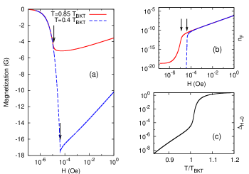
Figure 1: (Color online) (a)-(b) $M(H)$ and $n_{F}(H)$ below $T_{BKT}$ from the numerical solution of Eqs. (9)-(10). The arrows indicate $H_{c1}$ according to Eq. (14). At $T=0.4T_{BKT}$ $M(H)$ shows a sharp kink at $H_{c1}$, where $n_{F}$ drops abruptly to small values. At higher $T$ these features are partly smoothened out by thermal smearing. (c) Temperature dependence of the mass term $\Delta_{H=0}$. Notice that $\Delta_{H=0}\sim\Delta_{\Lambda}$ at $T_{BKT}$, where $\Lambda=6.9\times 10^{5}$ Å, $\Delta_{R}\sim 4\times 10^{-6}$ and $\Delta_{\Lambda}=1.9\times 10^{-5}$.

As a prototype of 2D system we consider a single layer of underdoped Bi2212, with $J(T)=J_{0}(1-T/T_{MF})$ to mimic the bare $T$ dependence due to quasiparticles, $J_{0}=180$ K and $T_{MF}=120$ K, which gives $T_{BKT}=84$ K. For $d=15$ Å as the typical interlayer distance the magnetization (8) is given in units of $k_{B}T/d\Phi_{0}=(4.4\times 10^{-3}T)$ G (or $(4.4\times T)$ A/m in the notation of Ref. Li et al. (2005)). Moreover, we use $R\sim 10^{6}a$ as the typical sample size, with $a=40$ Å, and choose $\mu=1.5\mu_{XY}$. With this choice of parameters one has always $R\gg\Lambda$ , so that $\Delta_{\Lambda}\sim 1/\Lambda\gg\Delta_{R}\sim 1/\sqrt{R\Lambda}$ up to $T_{BKT}$.

At $H=0$ Eq.s (9)-(10) are satisfied for $\tilde{M}=0$ and $\Delta$ solution of the equation $4Kg(\Delta_{H=0}+\Delta_{\Lambda})^{K}=\Delta_{H=0}^{2}$. At $\Delta_{\Lambda}=0$ the solution $\Delta_{H=0}^{2}=(4Kg)^{2/(2-K)}$ is finite only at $K<2$, which identifies the BKT transition at $K=2$ (i.e. $T_{BKT}=\pi J(T_{BKT})/2$). When a finite cut-off $\Delta_{\Lambda}$ is introduced $\Delta_{H=0}$ approaches $\Delta_{\Lambda}$ at $T_{BKT}$, and vanishes as $\Delta_{H=0}=\sqrt{4Kg}\Delta_{\Lambda}^{K/2}$ as $T\rightarrow 0$, giving $\Delta\ll\Delta_{\Lambda},\Delta_{R}$ already at $T\lesssim 0.9T_{BKT}$, see Fig. 1c. Observe that at $H=0$, where the same number of $\pm$ vortices are thermally-induced, $n=0$, and one can parametrize $n_{F}$ in Eq. (11) via the vortex correlation length $\xi$ as $1/\xi^{2}\equiv n_{F}/a^{2}=\Delta_{H=0}^{2}/4\pi Ka^{2}$.

At $H\neq 0$ a finite $\tilde{M}$ appears, which modifies also the $\Delta$ value. In general, at low field $\Delta$ keeps the zero-field value $\Delta(H)\approx\Delta_{H=0}$ and $\tilde{M}$ grows linearly with $H$. By further increasing $H$, $\Delta$ grows with respect to $\Delta_{H=0}$ and $\tilde{M}$ enters a non-linear regime. The slope of $M$ vs $H$, the absolute value of $\tilde{M}$ and the crossover field differ substantially above and below $T_{BKT}$. Let us first analyze the case $T<T_{BKT}$, i.e. $K>2$. For small $\tilde{M}$ one has $\tanh(\tilde{M})\approx\tilde{M}$ and $\cosh(\tilde{M})\approx 1$, so that we obtain $\tilde{M}=n_{H}(4\pi K)/(\Delta^{2}+\Delta_{R}^{2})$ and $\Delta(H)\approx\Delta_{H=0}$ from Eq. (10) and Eq. (9), respectively. Since $\Delta_{H=0}\ll(\Delta_{R},\Delta_{\Lambda})$ as $T\lesssim 0.9T_{BKT}$, and $\Delta_{R}^{2}\sim a^{2}/R\Lambda$, we obtain (using $8\pi^{2}Kk_{B}T/\Phi_{0}^{2}=1/\Lambda$):

$$M=-\frac{1}{4\pi}\frac{2R}{d}H,\quad n=n_{H}\frac{\Delta_{H=0}^{2}}{\Delta_{R}^{2}}\approx 0,$$ (12)

where we recognize flux expulsion ($n\equiv Ba^{2}/\Phi_{0}\approx 0$) and the Meissner effect ($-4\pi M=H/(1-\eta)$) in the presence of a large demagnetization factor $\eta\sim 1-d/R$ as expected in a thin filmLandau and Lifchitz (1984); Fetter and Hohenberg (1967). At large field instead $\cosh(\tilde{M})\approx e^{\tilde{M}}/2$ and $\tanh(\tilde{M})\approx 1$. We then obtain that $\tilde{M}\approx\log(2\Delta^{2-K}/p)$ from Eq. (9), and using $\Delta^{2}\approx 4\pi Kn_{H}$ from Eq. (10) we get:

$$M=-\frac{k_{B}T}{d\Phi_{0}}\left[A(T)+\left(\frac{T_{BKT}}{T}-1\right)\log\left(\frac{\Phi_{0}}{a^{2}H}\right)\right],$$ (13)

with $A(T)=\mu/k_{B}T-(K/2)\log(4\pi K)$. The linear regime (12) survives up to a field $H_{l}^{b}$ that can be determined by the numerical solution of Eqs. (9)-(10). As it is shown in Fig. 2b, $H_{l}^{b}$ is very low ($\sim 10^{-6}$ G) but finite at $T_{KT}$. For this reason, the field-independence of $M$ at criticality implied by Eq. (13) is only valid above $H_{l}^{b}$, below which $M\propto-H$, as expected. This low-field crossing to a linear behavior is missing in Ref. V. Oganesyan and Sondhi (2006) where $M$ is calculated as a function of $B$. However, at large fields where $B\approx H$ the dependence of $M(B)$ on $\log(B)$ derived there coincides with Eq. (13), apart from an additional $B$ dependence of $M$ at criticality that cannot be checked with the present variational calculation. Finally, we notice that at $T$ well below $T_{BKT}$ an estimate of $H_{l}^{b}$ can be obtained analytically by matching the high-field and low-field solutions for $\tilde{M}$ at $\Delta\approx\Delta_{\Lambda}$:

$$H_{c1}=\frac{\Phi_{0}}{4\pi}\frac{(\Delta_{R}/a)^{2}}{K}\left[(2-K)\log(2\Delta_{\Lambda})-\log(8Kg)\right],$$ (14)

which reduces for $T\rightarrow 0$ to the standard definition of first critical field in a SC film, $H_{c1}(T\rightarrow 0)=(\Phi_{0}/4\pi\Lambda R)\log(\Lambda/2a)+4\pi\mu/\Phi_{0}R$Fetter and Hohenberg (1967). Indeed, as we can see in Fig. 1a, at low $T$ the magnetization displays a sharp kink at $H_{c1}$ and increases just above it, as indeed expected at the threshold of flux penetration (see also $n_{F}$ in Fig. 1b). However, at higher temperatures such a kink in $M$ disappears due to thermal smearing and the minimum of $M$ is located at a field higher than $H_{c1}$.

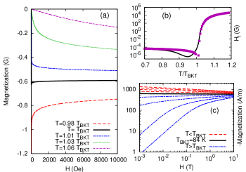
Figure 2: (Color online) (a) $M(H)$ above and below $T_{BKT}$ from the numerical solution of Eqs. (9)-(10). (b) Solid line: the threshold field $H_{l}^{a,b}$ as a function of $T$. The points show the analytical estimates (14)-(15), which agree with the numerical result except in a small range near $T_{BKT}$. (c) $M(H)$ in logarithmic scale (curves are spaced by 1K).

At $T>T_{BKT}$, i.e. $K<2$, $\tilde{M}$ shows again a crossover from a linear to non-linear behavior at a field $H_{l}^{a}$. To estimate $H_{l}^{a}$ we can expand the hyperbolic functions in Eq.s (9)-(10) around $\tilde{M}=0$. For $T$ sufficiently above $T_{BKT}$ so that $\Delta^{2}_{H=0}\simeq(4Kg)^{2/(2-K)}\gg(\Delta_{\Lambda},\Delta_{R})$ we obtain the approximate solutions $\tilde{M}=(4\pi Kn_{H})/\Delta^{2}$ and $\Delta^{2}=\Delta_{H=0}^{2}\left[1+1/({2-K})(H\xi/\Phi_{0})^{2}\right]$, where $\xi$ is the zero-field correlation length defined above. When the second term in the square brackets is $\ll 1$ the deviations of $\Delta^{2}$ with respect to $\Delta_{H=0}^{2}$ are negligible, so that

$$M=-\frac{k_{B}T}{d\Phi_{0}^{2}}\xi^{2}H,\,H\lesssim H_{l}^{a}=0.1\frac{\Phi_{0}}{\xi^{2}}\sqrt{\frac{T-T_{BKT}}{T}}$$ (15)

At $T$ sufficiently close to $T_{BKT}$ screening effects cut-off both $\Delta$ (i.e. $\xi$) and $H_{l}^{a}$, so that the estimate (15) is no more valid, $H_{l}^{a}$ attains a finite value and merges with the field $H_{l}^{b}$ discussed above, see Fig. 2b. As it was knownHalperin and Nelson (1979); V. Oganesyan and Sondhi (2006) the functional dependence of the low-field magnetization $M$ on the BKT correlation length $\xi$ in Eq. (15) is the same as in the GL theoryKoshelev (1994). However, the critical region $H<H_{l}^{a}$ where such a dependence is valid turns out to be remarkably smaller than in the standard GL theoryKoshelev (1994), because $\xi$ diverges much faster than in the GL case as $T\rightarrow T_{BKT}$.

In conclusion, we proposed a new theoretical framework to investigate the KT physics of 2D superconductors in a finite magnetic field, as given by the modified sine-Gordon model (6) and the definitions (3)-(5) of the physical quantities as a function of the applied magnetic field ${\bf H}$ (instead of ${\bf B}$). As we showed within a variational analysis of the model (6), we obtain a clear description of the Meissner phase below $T_{BKT}$, and an estimate of the threshold field $H_{l}^{a,b}$ for the appearance of non-linear effects. Above $T_{BKT}$ the shrinking of the linear regime with respect to standard GL fluctuations is a typical signature of the faster divergence of $\xi$ within the BKT theory. These results can shed new light on the physics of vortices in cuprates. Indeed, taking into account that in layered superconductors the intrinsic cut-off $R_{J}$ is provided by the interlayer coupling $J_{\perp}$ instead of $\Lambda$, $R_{J}\sim a\sqrt{J/J_{\perp}}$, our 2D calculations can be applied to these systems in all the $(T,H)$ range where $\Delta\gg 1/R_{J}$ (so that for example large demagnetization effects are not expected in layered systems). Thus, the persistence of a non-linear magnetization up to $H\sim 0.01$ T in a wide range of temperatures above $T_{BKT}$ found experimentally in Ref. Li et al. (2005) can be a signature of the rapid decreasing of $H_{l}^{a}$ as $T\rightarrow T_{BKT}$, which does not contradict but eventually support the KT nature of the SC fluctuations in these systems. Moreover, since $\xi$ increases as $\mu$ increases, the extremely low values of $H_{l}^{a}$ measured in Ref. Li et al. (2005) suggest a value of $\mu$ larger than $\mu_{XY}$, in agreement with the result of Ref. Benfatto et al. (2007) based on the analysis of the superfluid density, and call for a deeper investigation of the normal phase existing in the vortex cores.

References

- Berezinsky (1972) V. L. Berezinsky, Sov. Phys. JETP 34, 610 (1972); J. M. Kosterlitz and D. J. Thouless, J. Phys. C 6, 1181 (1973).
- Minnaghen (1987) P. Minnhagen, Rev. Mod. Phys. 59, 1001 (1987).
- Matthey et al. (2006) D. Matthey, et al., cond-mat/0603079.
- Crane et al. (2007) R. W. Crane, et al., Phys. Rev. B 75, 094506 (2007).
- Pourret et al. (2007) A. Pourret, et al., (2007), cond-mat/0701376.
- Hadzibabic et al. (2006) Z. Hadzibabic, et al., Nature 441, 1118 (2006).
- Li et al. (2005) L. Li, et al., Europhys. Lett. 72, 451 (2005).
- Cazalilla et al. (2007) M. A. Cazalilla, A. Iucci, and T. Giamarchi, Phys. Rev. A 75, 051603(R) (2007).
- Doniach and Huberman (1979) S. Doniach and B. A. Huberman, Phys. Rev. Lett. 42, 1169 (1979).
- Minnaghen (1981) P. Minnhagen, Phys. Rev. B 23, 5745 (1981).
- V. Oganesyan and Sondhi (2006) V. Oganesyan, D. A. Huse and S. L. Sondhi, Phys. Rev. B 73, 094503 (2006).
- Giamarchi (2004) T. Giamarchi, Quantum Physics in One Dimension (Oxford University Press, Oxford, 2004).
- Benfatto et al. (2007) L. Benfatto, C. Castellani, and T. Giamarchi, Phys. Rev. Lett. 98, 117008 (2007).
- Nandori (2007) I. Nandori, et al., J. Phys. Cond. Matt. 19, 236226 (2007). I. Nandori, et al., arXiv:0705.0578.
- Koshelev (1994) A. E. Koshelev, Phys. Rev. B 50, 506 (1994).
- José et al. (1977) J. José, et al., Phys. Rev. B 16, 1217 (1977).
- Landau and Lifchitz (1984) L. D. Landau and E. M. Lifchitz, Electrodynamics of Continuous Media (Pergamon, Oxford, 1984).
- Fetter and Hohenberg (1967) A. L. Fetter and P. C. Hohenberg, Phys. Rev. 159, 330 (1967).
- Halperin and Nelson (1979) B. I. Halperin and D. R. Nelson, J. Low. Temp. Phys. 36, 599 (1979).