Predictions for $\sin 2(\beta/\phi_{1})_{\rm eff}$ in $b\to s$ penguin dominated modes

Abstract

We provide a review of predictions for $\sin 2\beta_{\rm eff}$ in $b\to s$ penguin dominated modes based on $1/m_{b}$ expansion and/or SU(3) flavor symmetry. The experimental results are consistently lower than the theoretical predictions. In order to interpret whether this effect is a sign of new physics contributions or can be explained away within the Standard Model a theoretical input cannot be avoided. The effect survives at a level larger than $2.1\sigma$ in a conservative average over different modes that includes theoretical predictions.

I Introduction

A nontrivial test of the Standard Model (SM) are the two ways of measuring $\sin 2\beta$ from time dependent $\Delta S=1$ $B$ decays [with $\beta=\arg(-V_{cd}V^{*}_{cb}/V_{td}V^{*}_{tb})$]: (i) from tree dominated, e.g. $B\to J/\Psi K_{S}$ Bigi:1981qs , and (ii) from penguin dominated, e.g. $B\to\phi K_{S}$, decay modes London:1989ph ; Grossman:1996ke . The two determinations should be the same in the SM, but would differ, if new physics contributions modify the penguin dominated decay amplitudes. For several years now there is some disagreement between the two determinations, if the CKM suppressed terms are neglected in the interpretation of the experimental results. However, with the decreased experimental errors this approximation is no more adequate. As I will argue in this write-up theoretical input is needed for the correct interpretation of experimental results.

The two observables measured in time dependent $B(t)\to f$ decays into a CP eigenstate $f$ are the indirect CP asymmetry

$$S_{f}=2\frac{\rm{Im}\big{[}e^{-i2\beta}\bar{A}_{f}/{A_{f}}\big{]}}{1+|\bar{A}_{f}|^{2}/|{A_{f}}|^{2}},$$ (1)

and the direct CP asymmetry

$$C_{f}=\frac{|{A_{f}}|^{2}-|\bar{A}_{f}|^{2}}{|{A_{f}}|^{2}+|\bar{A}_{f}|^{2}}.$$ (2)

Above we have used the notation for the decay amplitudes $A(\bar{B}^{0}\to f)=\bar{A}_{f}$ and $A(B^{0}\to f)=A_{f}$. The choice of $\Delta S=1$ $B^{0}$ decays makes the determination of $\sin 2\beta$ from $S_{f}$ theoretically very clean since it exploits the CKM hierarchy $\lambda_{u}=V_{ub}V_{us}^{*}\sim\lambda^{2}\lambda_{c}$, where $\lambda_{c}=V_{cb}V_{cs}^{*}$ and $\lambda=\sin\theta_{C}=0.22$. To see this let us split the amplitude according to the CKM factors

$$\begin{split}\bar{A}_{f}&=\lambda_{c}a_{f}^{c}+\lambda_{u}a_{f}^{u}+\lambda_{t}a_{f}^{t}\\ &=\lambda_{c}(a_{f}^{c}-a_{f}^{t})+\lambda_{u}(a_{f}^{u}-a_{f}^{t})\\ &=\lambda_{c}A_{f}^{c}+\lambda_{u}A_{f}^{u},\end{split}$$ (3)

where in obtaining the second row the CKM unitarity $\lambda_{c}+\lambda_{u}+\lambda_{t}=0$ was used. The different terms in Eq. (3) can receive the following contributions, depending on the final state $f$: $a_{f}^{c}$ can receive contributions from $b\to c\bar{c}s$ tree and $c\bar{c}$ rescattering (charming penguin); $a_{f}^{u}$ can receive contributions from $b\to u\bar{u}s$ tree and $u\bar{u}$ rescattering ($u-$penguin); $a_{f}^{t}$ can receive contributions from QCD penguins and electroweak penguins.

Since $\lambda_{u}\sim 0.02\lambda_{c}$ there is a big hierarchy between the two terms in $\bar{A}_{f}=\lambda_{c}A_{f}^{c}+\lambda_{u}A_{f}^{u}$, so that $\bar{A}_{f}$ is dominated by one CKM amplitude. Since $\lambda_{c}$ is real in the standard CKM parametrisation, $\bar{A}_{f}\simeq A_{f}$, and the ratio of the two amplitudes cancels to first approximation in Eq. (1). More precisely, expanding in the small ratio

$$r_{f}e^{i\delta_{f}}=\left|{\lambda_{u}}/{\lambda_{c}}\right|\cdot\frac{A_{f}^{u}}{A_{f}^{c}}\simeq 0.02\frac{A_{f}^{u}}{A_{f}^{c}},$$ (4)

we have

$$\begin{split}\sin 2\beta_{\rm eff}&\equiv-\eta_{f}^{CP}S_{f}=\\ &=\sin 2\beta+2r_{f}\cos\delta_{f}\cos 2\beta\sin\gamma,\end{split}$$ (5)

where $\eta_{f}^{CP}$ is the CP of the final state $f$, and

$$C_{f}=-2r_{f}\sin\delta_{f}\sin\gamma.$$ (6)

If the small $r_{f}$ terms are neglected we thus have $\sin 2\beta_{\rm eff}=\sin 2\beta$ and $C_{f}=0$. If a nonzero direct CP asymmetry $C_{f}$ is found experimentally, it would immediately imply that $r_{f}$ terms are important.

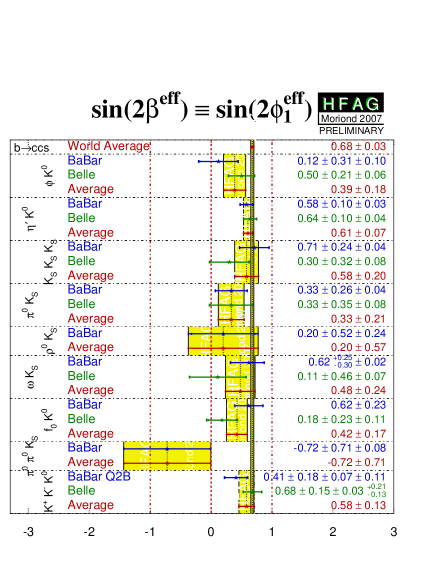
Figure 1: The measured $\sin 2\beta_{\rm eff}^{\rm Peng}$ for $\Delta S=1$ penguin dominated decays Barberio:2007cr . The two vertical yellow lines give the $\sin 2\beta_{\rm eff}^{\rm Tree}$ from $b\to c\bar{c}s$ world average.

II Two ways to $\sin 2\beta$

As alluded to in the introduction, it is useful to distinguish two determinations of $\sin 2\beta$. The tree dominated decays, e.g. $B^{0}\to J/\Psi K_{S}$, are expected to be SM dominated. We will denote the corresponding value in Eq. (5) as $\sin 2\beta_{\rm eff}^{\rm Tree}$. The penguin dominated decays, e.g. $B^{0}\to\phi K_{S}$, can on the contrary receive possibly large beyond Standard Model contributions. The corresponding values in Eq. (5) will be denoted as $\sin 2\beta_{\rm eff}^{\rm Peng}$. The comparison of the two then tests the KM mechanism

$$\begin{split}\Delta S_{f}&=\sin 2\beta_{\rm eff}^{\rm Peng}-\sin 2\beta_{\rm eff}^{\rm Tree}\\ &=O(r_{f}^{\rm Peng})-O(r_{f}^{\rm Tree}).\end{split}$$ (7)

The $O(r_{f}^{\rm Tree})$ difference between $\sin 2\beta$ and $S_{J/\Psi K_{S}}$ is below a percent level, since $A_{f}^{u}$ in Eq. (4) is already at least $\alpha_{S}(m_{b})$ suppressed compared to the dominant tree term, $A_{f}^{c}$ Gronau:1989ia ; Boos:2004xp ; Ciuchini:2005mg ; Li:2006vq . These $O(r_{f}^{\rm Tree})$ corrections will be neglected compared to the $O(r_{f}^{\rm Peng})$ differences between $\sin 2\beta_{\rm eff}^{\rm Peng}$ and $\sin 2\beta$ which we will investigate below.

The expected difference $\Delta S_{f}$ for penguin dominated modes is channel dependent. Curiously enough, the experimental values are all negative, $\Delta S_{f}<0$, see Fig. 1. This experimental pattern immediately raises several questions

• what are the SM expectations?

• what are the errors on the theory predictions?

• what theoretical errors to expect in the future/can we improve them?

The last question is especially interesting for future prospects, where with 50 ab^-1 of data $S_{\phi K_{S}}$ and $S_{\eta^{\prime}K_{S}}$ are expected to be measured to a precision of a few percent.

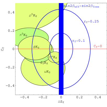
Figure 2: The $1\sigma$ experimental values for ($\Delta S_{f},C_{f}$) in penguin dominated modes as of FPCP07 conference Barberio:2007cr . The vertical blue band shows experimental errors on $\sin 2\beta_{\rm eff}^{\rm Tree}$ from $b\to c\bar{c}s$ modes. The two blue circles represent $\Delta S_{f}$ for $r_{f}=0.1,0.25$ with $\delta_{f}$ varied (with $\gamma=60^{\circ}$).

An important thing to note is that we have 2 observables, $S_{f}$ and $C_{f}$, but also 2 unknowns: $\sin\gamma~{}r_{f}$ and $\delta_{f}$

$$\Delta S_{f} =2\sin\gamma~{}r_{f}\cos\delta_{f}\cos 2\beta$$ (8)

$$C_{f} =-2\sin\gamma~{}r_{f}\sin\delta_{f}$$ (9)

To predict $\Delta S_{f}$ one therefore necessarily needs theory input at least on $r_{f}$, while $\delta_{f}$ could in principle be fixed from a measurement of $C_{f}$ (or vice versa). An example of this is shown in Fig. 2, where the experimental results are compared with ellipses in $(\Delta S_{f},C_{f})$ plane obtained for $r_{f}=0.1,0.25$ and arbitrary $\delta_{f}$ (and with $\gamma$ chosen to be $60^{\circ}$). Note that these two values of $r_{f}$ correspond to fairly large values of $A_{f}^{u}/A_{f}^{c}\sim 5,10$ in Eq. (4).

Both $\Delta S_{f}$ and $C_{f}$ have been estimated in several theoretical frameworks using SU(3) flavor symmetry and using $1/m_{b}$ expansion: QCDF, SCET, pQCD. We discuss these two approaches next.

III Using flavor SU(3)

As pointed out in Grossman:2003qp and discussed later also in Gronau:2004hp ; Gronau:2003kx ; Gronau:2006qh ; Gronau:2005gz ; Raz:2005hu ; Engelhard:2005ky ; Engelhard:2005hu one can use $\Delta S=0$ modes related by $SU(3)_{F}$ (represented by $s\to d$ exchange on Fig. 3) to constrain $\Delta S_{f}$ in penguin dominated $\Delta S=1$ decays. This corresponds to a replacement $V_{cb}V_{cs}^{*}A_{f}^{c}\to V_{cb}V_{cd}^{*}A_{f}^{c}{}^{\prime}$ and $V_{ub}V_{us}^{*}A_{f}^{u}\to V_{ub}V_{ud}^{*}A_{f}^{u}{}^{\prime}$ in Eq. (3), where the primes remind us of the fact that one needs to take into account SU(3) breaking as well as of the fact that $f$ may transform into a sum of mass eigenstates (for instance U-spin transforms $\pi^{0}\sim(u\bar{u}-d\bar{d})/\sqrt{2}$ to $(u\bar{u}-s\bar{s})/\sqrt{2}$, which is a sum of $\eta$ and $\eta^{\prime}$).

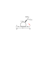
Figure 3: The $s\to d$ exchange modifies the hierarchy of tree (left diagram) and penguin (right diagram) contributions by replacing $V_{ts}\to V_{td}$ and $V_{us}\to V_{ud}$ respectively.

In the SU(3) related amplitudes the hierarchy of tree and penguin contributions is changed because the CKM factors in front of the matrix elements $A_{f}^{c,u}$ in Eq. (3) have changed

$$P\to-\lambda P^{\prime},\quad T\to T^{\prime}/\lambda.$$ (10)

For instance, the $B\to\pi K$ amplitudes are penguin dominated, while in SU(3) related $B\to\pi\pi$ decays the tree contributions are larger than the penguins. Because of this, one can bound ”tree pollution” $r_{f}$ in $\Delta S=1$ decays from the related $\Delta S=0$ modes. A bound on $r_{f}$ consists of a sum over modes

$$r_{f}\leq\frac{{\cal R}+\bar{\lambda}^{2}}{1-{\cal R}},\quad{\cal R}\leq\bar{\lambda}\sum_{f^{\prime}}|a_{f^{\prime}}|\sqrt{\frac{\bar{\cal B}_{f^{\prime}}(\Delta S=0)}{\bar{\cal B}_{f}(\Delta S=1)}},$$ (11)

where $a_{f^{\prime}}$ are numerical coefficients. From the above equation we immediately see that the bound can never be better than $r_{f}<\bar{\lambda}^{2}\sim 0.05$, even if ${\cal R}$ is set to zero.

The upper bound on ${\cal R}$ in Eq. (11) was obtained by bounding a sum over amplitudes, where there would be in general cancellations between different terms, with a sum over absolute values of amplitudes, where of course no such cancellations occur. The bound on ${\cal R}$ is thus in general better, if the sum is over a smaller set of modes $f^{\prime}$. Furthermore, all the branching ratios $f^{\prime}$ in the bound need to be measured to have the best bound. At present for some $\Delta S=0$ modes only upper bounds are known. For instance in the bound on $r_{\eta^{\prime}K_{S}}$ the branching ratios for $B^{0}\to\pi^{0}\eta,\eta^{(^{\prime})}\eta^{(^{\prime})}$ decays enter. For these only experimental upper bounds exist, giving at present ${\cal R}_{\eta^{\prime}K_{S}}<0.116$, while one arrives at ${\cal R}<0.045$, if the predicted branching ratio in QCDF, Scenario 4, are used (or ${\cal R}<0.088$ if SCET, Sol. I., predictions are used). Clearly, there is still room for improvement using this approach. But in general, assuming only SU(3) without any dynamical assumptions, gives too conservative bounds. The reason is that in this way one does not use any information about the relative phases between the terms in the sum in Eq. (11). The results of a 2006 numerical update Gronau:2006qh , where correlations between $S_{f}$ and $C_{f}$ were used, are shown on Fig. 4. Bounds on $\Delta S_{\phi K_{S}}$ are much worse Grossman:2003qp . It is also possible to treat $S_{KKK}$ in this framework, however, the bounds are again not very informative Engelhard:2005ky ; Engelhard:2005hu . Assuming small annihilation one has $r_{K^{+}K^{-}K^{0}}<1.02,$ and $r_{K_{S}K_{S}K_{S}}<0.31$ Engelhard:2005ky ; Engelhard:2005hu .

Another use of SU(3) is to perform global fits to the data Chiang:2003pm ; Chiang:2004nm ; Buras:2003dj ; Fleischer:2007mq . In this case $\Delta S_{f}$ can be predicted and not just bounded as above. A recent analysis in Fleischer:2007mq shows a discrepancy between experimental data and the SU(3) fit predictions in the $(S_{\pi^{0}K_{S}},C_{\pi^{0}K_{S}})$ plane. The fit predicts $S_{\pi^{0}K_{S}}=-0.81\pm 0.03$ in the Standard Model, which is to be compared with the measured value of $S_{\pi^{0}K_{S}}=-0.33\pm 0.21$. Note that the error on the prediction already includes the variation due to the SU(3) breaking.

Figure 4: Top: $(S_{\eta^{\prime}K_{S}},C_{\eta^{\prime}K_{S}})$ values allowed by SU(3) bounds (region enclosed by the solid curve), and with further dynamical assumptions (region enclosed by the dashed curve) Gronau:2006qh . Bottom: $(S_{\pi^{0}K_{S}},C_{\pi^{0}K_{S}})$ values allowed by SU(3) bounds Gronau:2006qh . The small points are $(S_{f},C_{f})=(\sin 2\beta,0)$. Experimental values are from BaBar (dot) Aubert:2006wv ; Aubert:2006ad and from Belle (square) Chen:2006nk ; Hara:Belle .

IV Using $1/m_{b}$ expansion

The $1/m_{b}$ expansion has more predictive power. I would like to stress that $1/m_{b}$ expansion is a consistent framework, based on Soft Collinear Effective Theory Bauer:2000ew . Like the SU(3) approach it is in principle ”model independent” in the sense that it uses only symmetries of QCD. While the SU(3) approach uses a symmetry that arises in the $m_{s}\to 0$ limit, SCET based approaches use the symmetry that arise in the $m_{b}\to\infty$ limit. The framework offers consistency checks both within two-body $B$ decays as well as in $B\to D\pi$ Mantry:2003uz and semiinclusive hadronic decays Chay:2006ve ; Soni:2005jj . Note that both QCD Factorization (QCDF) Beneke:1999br ; Beneke:2002jn ; Beneke:2003zv and the so-called SCET calculations Bauer:2004tj ; Jain:2007dy ; Williamson:2006hb use Soft Collinear Effective Theory, but they differ in the treatment of subleading effects and charming penguin contributions Bauer:2005wb ; Beneke:2004bn .

We first review state of the art in these calculations and then move on to the predictions in specific decay modes. Both in QCDF and SCET the hard kernels are known to NLO in $\alpha_{S}(m_{b})$ Beneke:1999br ; Chay:2003ju ; Jain:2007dy ; Beneke:2005vv , with partial results already known at NNLO Bell:2007tv . The jet functions are known to NLO in $\alpha_{S}(\sqrt{\Lambda m_{b}})$ Hill:2004if ; Kirilin:2005xz ; Beneke:2005gs . At present the limit on accuracy is the inclusion of $1/m_{b}$ corrections. While some of them, for instance the chirally enhanced terms, have already been included Beneke:1999br ; Jain:2007dy , more work is needed to complete the calculations to $1/m_{b}$ order.

Not all of this information was used in $\Delta S_{f}$ calculations, however. In most recent QCDF calculation of Ref. Beneke:2005pu hard scattering was treated at LO in $\alpha_{S}(m_{b})$, $\alpha_{S}(\sqrt{\Lambda m_{b}})$, soft overlap at NLO in $\alpha_{S}(m_{b})$ and some $1/m_{b}$ corrections were included (modeled). In SCET calculation Williamson:2006hb all hard kernels were taken at LO in $\alpha_{S}(m_{b})$, jet functions were not expanded in $\alpha_{S}(\sqrt{\Lambda m_{b}})$, $1/m_{b}$ corrections were not included, while nonperturbative parameters (also the charming penguin one, $P_{\rm charm}$) were fit from data. In pQCD calculations Li:2005kt ; Li:2006jv the soft overlap contribution is factorized and some NLO corrections are included.

An interesting way of using the $1/m_{b}$ expansion results was proposed by M. Ciuchini et al. Ciuchini:2001gv ; Silvestrini:2007yf . Here the renormalization group invariant parametrization of the decay amplitudes Buras:1998ra is used to fit from data the $1/m_{b}$ corrections to the QCDF predictions. In this way a better desription of branching ratios and CP asymmetries is obtained. The predictions on $\Delta S_{f}$ are compatible with the original QCDF predictions, albeit with larger errors Silvestrini:2007yf . The errors will shrink once more data on relevant branching ratios and direct CP asymmetries become available.

IV.1 $\Delta S$ for $\phi K_{S}$

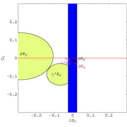
Figure 5: Crosses: QCDF (black) Beneke:2003zv , pQCD(red) Li:2006vq , and SCET (magenta) Williamson:2006hb predictions for $\Delta S_{f},C_{f}$, with $f=\phi K_{S},\eta^{\prime}K_{S}$. Ellipses are experimental $1\sigma$ allowed regions, blue band is experimental error on $\sin 2\beta$ from $b\to c\bar{c}s$.

This is the cleanest mode, with the least ambiguity on $\Delta S_{f}$, since there is no $b\to u\bar{u}s$ tree contribution. One thus has

$$\frac{A_{f}^{u}}{A_{f}^{c}}=\frac{a_{f}^{u}-a_{f}^{t}}{a_{f}^{c}-a_{f}^{t}}\sim O(1),$$ (12)

where $a_{f}^{i}$ are either $\alpha_{S}(m_{b})$ (penguins) or $1/m_{b}$ suppressed. The ”tree pollution” parameter $r_{f}$ is then at a percent level as demanded by the CKM suppression, $r_{f}\simeq 0.02{A_{f}^{u}}/{A_{f}^{c}}$. In particular, the ratio of the matrix elements, ${A_{f}^{u}}/{A_{f}^{c}}$, cannot be enhanced, since there is no tree contribution to ${A_{f}^{u}}$. In accordance with this expectation both calculations in QCDF Beneke:2005gs and pQCD Li:2006jv obtain

$$\Delta S_{\phi K_{S}}=0.02\pm 0.01,$$ (13)

while there is no prediction in SCET yet. An analysis in Cheng:2005bg suggest that final state interactions do not change the above result.

IV.2 $\Delta S$ for $\eta^{\prime}K_{S}$

Because $\eta^{\prime}$ contains a $u\bar{u}$ component there is a $b\to u\bar{u}s$ tree level contribution to the $B\to\eta K_{S}$ decay amplitude. However, $r_{f}$ is still small, since $A_{f}^{c}$ is also enhanced. This enhanced $A_{f}^{c}$ explains the large $Br(B\to\eta^{\prime}K_{S})$ observed experimentally. The enhancement itself can be understood through constructive interference between $A(B\to\eta_{q}K_{S})$ and $A(B\to\eta_{s}K_{S})$, a mechanism that also explains small $Br(B\to\eta K_{S})$, where the interference is destructive Lipkin:1990us ; Lipkin:1998ew . Besides the interference pattern gluonic contributions and/or SU(3) breaking are needed to obtain the experimentally observed branching ratios Beneke:2002jn ; Beneke:2003zv ; Gerard:2006ch ; Williamson:2006hb .

The nonperturbative parameters including gluonic charming penguins were fit from experimental data in SCET Williamson:2006hb (but not from $\Delta S_{\eta^{\prime}K_{S}}$, which is a pure prediction), while in QCDF calculation of Beneke:2003zv a reasonable estimate for these unknown terms was used. The two predictions

$$\begin{split}{\rm QCDF:~{}}\Delta S_{\eta^{\prime}K_{S}}=&0.01\pm 0.01,\\ {\rm SCET:~{}}\Delta S_{\eta^{\prime}K_{S}}=&\left\{\begin{matrix}-0.019\pm 0.008,{\rm~{}Sol.~{}I},\\ -0.010\pm 0.010,{\rm~{}Sol.~{}II},\end{matrix}\right.\end{split}$$ (14)

do not coincide, but both of them do consistently give small deviations. This would be true also if, for some reason, the strong phases between $A^{c}$ and $A^{u}$ were completely missed in the calculation, since $|A^{u}/A^{c}|$ is $O(1)$ as in $B\to\phi K_{S}$, Eq. (12), and is not enhanced despite the presence of a tree contribution. The situation is reversed in $B\to\eta K_{S}$, where the destructive interference between $A(B\to\eta_{q}K_{S})$ and $A(B\to\eta_{s}K_{S})$ suppresses $A_{f}^{c}$ and makes the tree contribution relatively larger. Then $\Delta S_{\eta K_{S}}$ can be large, even $O(1)$.

IV.3 Other 2-body modes

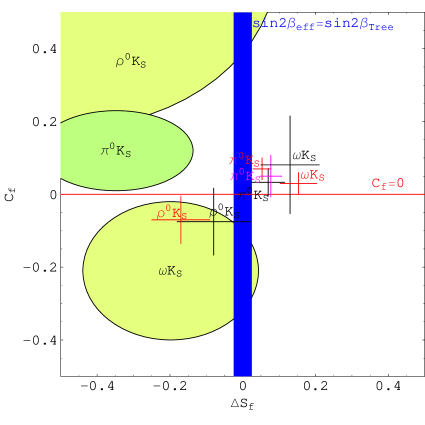
Figure 6: Crosses: QCDF (black) Beneke:2003zv , pQCD(red) Li:2006vq ; Li:2005kt , and SCET (magenta) Williamson:2006hb predictions for $\Delta S_{f},C_{f}$. Ellipses are experimental $1\sigma$ allowed regions, blue band is experimental error on $\sin 2\beta$ from $b\to c\bar{c}s$.

The other 2-body modes for which there exist predictions on $\Delta S_{f}$ are ${\pi^{0}K_{S}}$, ${\rho^{0}K_{S}}$ and ${\omega K_{S}}$. All of these receive $b\to u\bar{u}s$ tree contributions, so that $A^{u}$ is enhanced over $A^{c}$. In general one expects $\Delta S_{f}$ $\sim O(0.1)$, with calculated values given below

Mode	QCDF Beneke:2005pu	pQCD Li:2006vq ; Li:2005kt	SCET Williamson:2006hb
${\pi^{0}K_{S}}$	$0.07^{+0.05}_{-0.04}$	$0.053^{+0.02}_{-0.03}$	$0.077\pm 0.030$
${\rho^{0}K_{S}}$	$-0.08^{+0.08}_{-0.12}$	$-0.187^{+0.10}_{-0.06}$	$-$
${\omega K_{S}}$	$0.13\pm 0.08$	$0.153^{+0.03}_{-0.07}$	$-$

It is interesting to note that $\Delta S_{\rho K_{S}}$ is the only one that is predicted to be negative, while all experimental central values are negative (see Fig. 6). According to the analysis Cheng:2005bg final state interactions could change appreciably $S_{\omega K_{S}}$, $S_{\rho K_{S}}$, but even then one still has $\Delta S_{f}$ $\sim O(0.1)$.

V Three-body modes

In Gershon:2004tk it was noted that $B\to\pi^{0}\pi^{0}K_{S}$ and $B\to K_{S}K_{S}K_{S}$ are CP-even over the entire phase space so that no dilution of $S_{f}$ occurs in the integration over the phase space. This nice property does not hold for $B\to K^{+}K^{-}K_{S}$ where both CP-even and CP-odd components are present. Nevertheless, an analysis based on isospin shows that $B\to K^{+}K^{-}K_{S}$ away from $\phi K_{S}$ is mostly CP even Gronau:2005ax ; Garmash:2003er .

Since there are no $b\to u\bar{u}s$ tree contributions in $B\to K_{S}K_{S}K_{S}$ one would naively expect $\Delta S_{K_{S}K_{S}K_{S}}$ to be very small, and for the other $\Delta S_{KKK}$ to be $\sim O(0.1)$. However, a calculation based on HM$\chi$PT, a model of form factors and a model of non-resonant amplitude behaviour gives all $\Delta S_{f}\sim 0.05$ Cheng:2005ug ; Cheng:2007si . More work is needed to confirm this observation.

VI Conclusions

The experimental values of $\Delta S_{f}$ are found to be negative in all modes and are also consistently lower than the theoretical predictions. It is a bit more difficult to assign a statistical significance to this statement, however. It is clear that different decay modes have different ”tree pollutions”, with $\phi K_{S}$ and $\eta^{\prime}K_{S}$ being the cleanest. Simply averaging the experimental values for $\Delta S_{f}$ over different modes is not correct, since the ”tree pollution” is not negligible compared to the experimental errors. To ascertain whether the experimental values of $\Delta S_{f}$ represent a deviation from SM or not the use of theory therefore cannot be avoided.

The question is: how to take into account the theory? If all three approaches, QCDF, SCET and pQCD gave identical predictions, there would have been no problem. While this is not the case, the three approaches do give comparable predictions for different modes, with the difference attributable to different treatments of higher order corrections. None of the treatments thus seems to be clearly wrong either.

I would like to advertise two prescriptions that are both conservative and fairly intuitive. The first one is to take the theoretical framework in which the largest number of predictions has been made and only average over modes where there are theoretical predictions, while dropping the remaining experimental results (alas!). The largest set of predictions for different modes is at present available in QCDF Beneke:2005pu . Taking the lowest $(\Delta S_{f})_{\rm Th}$ value obtained in the scan over QCDF input parameters in Beneke:2005pu and then averaging the difference

$$(\Delta{S_{f}})_{\rm Corr}=(\Delta S_{f})_{\rm Exp}-(\Delta S_{f})_{\rm Th},$$ (15)

by using only the experimental errors, gives

$$\begin{split}\overline{(\Delta{S_{f}})}_{\rm Corr}&=\sin 2\beta^{\rm Peng}-\sin 2\beta^{\rm Tree}\\ &=-0.133\pm 0.063\quad(>2.1\sigma{\rm~{}effect}).\end{split}$$ (16)

In the above average the $3-$body modes and the $f_{0}K_{S}$ mode were dropped since there are no predictions for the corresponding $S_{f}$ in QCDF. The error in Eq. (16) does not have a clear statistical meaning. Nevertheless, I believe the correct interpretation of the above result is that we have an effect that is larger than $0.133/0.063=2.1$ $\sigma$.

The other conservative prescription is that for each $(\Delta{S_{f}})_{\rm Corr}$ one takes the smallest value predicted from the three theoretical approaches, QCDF, SCET and pQCD, and then averages over modes while adding quadratically theoretical and experimental errors. Curiously enough this gives at present almost exactly the same result as quoted for the first prescription in Eq. (16) above.

- (1) I. I. Y. Bigi and A. I. Sanda, Nucl. Phys. B 193, 85 (1981).
- (2) D. London and R. D. Peccei, Phys. Lett. B 223, 257 (1989).
- (3) Y. Grossman and M. P. Worah, Phys. Lett. B 395, 241 (1997) [arXiv:hep-ph/9612269].
- (4) E. Barberio et al. [Heavy Flavor Averaging Group (HFAG) Collaboration], arXiv:0704.3575 [hep-ex] and online update at http://www.slac.stanford.edu/xorg/hfag
- (5) M. Gronau, Phys. Rev. Lett. 63, 1451 (1989).
- (6) H. Boos, T. Mannel and J. Reuter, Phys. Rev. D 70, 036006 (2004) [arXiv:hep-ph/0403085].
- (7) M. Ciuchini, M. Pierini and L. Silvestrini, Phys. Rev. Lett. 95, 221804 (2005) [arXiv:hep-ph/0507290].
- (8) H. n. Li and S. Mishima, JHEP 0703, 009 (2007) [arXiv:hep-ph/0610120].
- (9) Y. Grossman, Z. Ligeti, Y. Nir and H. Quinn, Phys. Rev. D 68, 015004 (2003) [arXiv:hep-ph/0303171].
- (10) M. Gronau, J. L. Rosner and J. Zupan, Phys. Lett. B 596, 107 (2004) [arXiv:hep-ph/0403287].
- (11) M. Gronau, Y. Grossman and J. L. Rosner, Phys. Lett. B 579, 331 (2004) [arXiv:hep-ph/0310020].
- (12) M. Gronau, J. L. Rosner and J. Zupan, Phys. Rev. D 74, 093003 (2006) [arXiv:hep-ph/0608085].
- (13) M. Gronau and J. L. Rosner, Phys. Rev. D 71, 074019 (2005) [arXiv:hep-ph/0503131].
- (14) G. Raz, arXiv:hep-ph/0509125.
- (15) G. Engelhard and G. Raz, Phys. Rev. D 72, 114017 (2005) [arXiv:hep-ph/0508046].
- (16) G. Engelhard, Y. Nir and G. Raz, Phys. Rev. D 72, 075013 (2005) [arXiv:hep-ph/0505194].
- (17) C. W. Chiang, M. Gronau, Z. Luo, J. L. Rosner and D. A. Suprun, Phys. Rev. D 69, 034001 (2004) [arXiv:hep-ph/0307395].
- (18) C. W. Chiang, M. Gronau, J. L. Rosner and D. A. Suprun, Phys. Rev. D 70, 034020 (2004) [arXiv:hep-ph/0404073].
- (19) A. J. Buras, R. Fleischer, S. Recksiegel and F. Schwab, Phys. Rev. Lett. 92, 101804 (2004) [arXiv:hep-ph/0312259]; Nucl. Phys. B 697, 133 (2004) [arXiv:hep-ph/0402112]; Eur. Phys. J. C 45, 701 (2006) [arXiv:hep-ph/0512032].
- (20) R. Fleischer, S. Recksiegel and F. Schwab, Eur. Phys. J. C 51, 55 (2007) [arXiv:hep-ph/0702275].
- (21) B. Aubert et al. [BABAR Collaboration], Phys. Rev. Lett. 98, 031801 (2007) [arXiv:hep-ex/0609052].
- (22) B. Aubert et al. [BABAR Collaboration], arXiv:hep-ex/0607096.
- (23) K. F. Chen et al. [Belle Collaboration], Phys. Rev. Lett. 98, 031802 (2007) [arXiv:hep-ex/0608039].
- (24) K. Hara [Belle Collaboration], presented at ICHEP06, Moscow.
- (25) C. W. Bauer, S. Fleming and M. E. Luke, Phys. Rev. D 63, 014006 (2001) [arXiv:hep-ph/0005275]. C. W. Bauer, S. Fleming, D. Pirjol and I. W. Stewart, Phys. Rev. D 63, 114020 (2001) [arXiv:hep-ph/0011336]; C. W. Bauer and I. W. Stewart, Phys. Lett. B 516, 134 (2001) [arXiv:hep-ph/0107001].
- (26) S. Mantry, D. Pirjol and I. W. Stewart, Phys. Rev. D 68, 114009 (2003) [arXiv:hep-ph/0306254].
- (27) A. Soni and J. Zupan, Phys. Rev. D 75, 014024 (2007) [arXiv:hep-ph/0510325].
- (28) J. Chay, C. Kim, A. K. Leibovich and J. Zupan, Phys. Rev. D 74, 074022 (2006) [arXiv:hep-ph/0607004].
- (29) M. Beneke, G. Buchalla, M. Neubert and C. T. Sachrajda, Phys. Rev. Lett. 83, 1914 (1999) [arXiv:hep-ph/9905312]; Nucl. Phys. B 591, 313 (2000) [arXiv:hep-ph/0006124]; M. Beneke, G. Buchalla, M. Neubert and C. T. Sachrajda, Nucl. Phys. B 606, 245 (2001) [arXiv:hep-ph/0104110].
- (30) M. Beneke and M. Neubert, Nucl. Phys. B 651, 225 (2003) [arXiv:hep-ph/0210085].
- (31) M. Beneke and M. Neubert, Nucl. Phys. B 675, 333 (2003) [arXiv:hep-ph/0308039].
- (32) C. W. Bauer, D. Pirjol, I. Z. Rothstein and I. W. Stewart, Phys. Rev. D 70, 054015 (2004) [arXiv:hep-ph/0401188]; C. W. Bauer, I. Z. Rothstein and I. W. Stewart, Phys. Rev. D 74, 034010 (2006) [arXiv:hep-ph/0510241].
- (33) A. Jain, I. Z. Rothstein and I. W. Stewart, arXiv:0706.3399 [hep-ph].
- (34) A. R. Williamson and J. Zupan, Phys. Rev. D 74, 014003 (2006) [arXiv:hep-ph/0601214].
- (35) C. W. Bauer, D. Pirjol, I. Z. Rothstein and I. W. Stewart, Phys. Rev. D 72, 098502 (2005) [arXiv:hep-ph/0502094].
- (36) M. Beneke, G. Buchalla, M. Neubert and C. T. Sachrajda, Phys. Rev. D 72, 098501 (2005) [arXiv:hep-ph/0411171].
- (37) J. Chay and C. Kim, Nucl. Phys. B 680, 302 (2004) [arXiv:hep-ph/0301262].
- (38) M. Beneke and S. Jager, Nucl. Phys. B 751, 160 (2006) [arXiv:hep-ph/0512351]; M. Beneke and S. Jager, Nucl. Phys. B 768, 51 (2007) [arXiv:hep-ph/0610322].
- (39) G. Bell, arXiv:0705.3127 [hep-ph].
- (40) R. J. Hill, T. Becher, S. J. Lee and M. Neubert, JHEP 0407, 081 (2004) [arXiv:hep-ph/0404217].
- (41) G. G. Kirilin, arXiv:hep-ph/0508235.
- (42) M. Beneke and D. Yang, Nucl. Phys. B 736, 34 (2006) [arXiv:hep-ph/0508250].
- (43) M. Beneke, Phys. Lett. B 620, 143 (2005) [arXiv:hep-ph/0505075].
- (44) H. n. Li, S. Mishima and A. I. Sanda, Phys. Rev. D 72, 114005 (2005) [arXiv:hep-ph/0508041].
- (45) H. n. Li and S. Mishima, Phys. Rev. D 74, 094020 (2006) [arXiv:hep-ph/0608277].
- (46) M. Ciuchini, E. Franco, G. Martinelli, M. Pierini and L. Silvestrini, Phys. Lett. B 515, 33 (2001) [arXiv:hep-ph/0104126].
- (47) L. Silvestrini, arXiv:0705.1624 [hep-ph].
- (48) A. J. Buras and L. Silvestrini, Nucl. Phys. B 569, 3 (2000) [arXiv:hep-ph/9812392].
- (49) H. Y. Cheng, C. K. Chua and A. Soni, Phys. Rev. D 72, 014006 (2005) [arXiv:hep-ph/0502235].
- (50) H. J. Lipkin, Phys. Lett. B 254, 247 (1991).
- (51) H. J. Lipkin, Phys. Lett. B 433, 117 (1998).
- (52) J. M. Gerard and E. Kou, Phys. Rev. Lett. 97, 261804 (2006) [arXiv:hep-ph/0609300].
- (53) T. Gershon and M. Hazumi, Phys. Lett. B 596, 163 (2004) [arXiv:hep-ph/0402097].
- (54) M. Gronau and J. L. Rosner, Phys. Rev. D 72, 094031 (2005) [arXiv:hep-ph/0509155].
- (55) A. Garmash et al. [Belle Collaboration], Phys. Rev. D 69, 012001 (2004) [arXiv:hep-ex/0307082].
- (56) H. Y. Cheng, C. K. Chua and A. Soni, Phys. Rev. D 72, 094003 (2005) [arXiv:hep-ph/0506268].
- (57) H. Y. Cheng, C. K. Chua and A. Soni, arXiv:0704.1049 [hep-ph].