Construction and test of a moving boundary model for negative streamer discharges

Abstract

Starting from the minimal model for the electrically interacting particle densities in negative streamer discharges, we derive a moving boundary approximation for the ionization fronts. The boundary condition on the moving front is found to be of ’kinetic undercooling’ type. The boundary approximation, whose first results have been published in [Meulenbroek et al., PRL 95, 195004 (2005)], is then tested against 2-dimensional simulations of the density model. The results suggest that our moving boundary approximation adequately represents the essential dynamics of negative streamer fronts.

I Introduction

Streamers are growing plasma channels extending in strong electric fields through large volumes of matter; they determine the initial stages of electric breakdown equally in technical and natural processes Raether ; Loeb ; Raizer ; PSST . Negative (anode-directed) streamers, which are the subject of this work, can be described on a mesoscopic level by a system of reaction advection diffusion equations for electron and ion densities coupled to the electric field. Numerical solutions Kunhardt ; dhal85 ; dhal87 ; vite94 ; PRLMan ; AndreaRapid ; CaroAva ; CaroRapid ; CaroJCP of this minimal model reveal that the evolution of the streamer channel is dominated by a space charge layer forming around the tip. This layer enhances the electric field in front of the streamer, which leads to rapid growth through an efficient impact ionization by field accelerated electrons. It furthermore screens the electric field from the streamer bulk. Fig. 1 illustrates the development of this space charge layer, starting from a smooth initial ionization seed. More detailed illustrations of fully developed streamer fronts will be presented in Sec. IV. In the fully developed streamer, the width of the space charge layer is much smaller than the radius of the streamer head; this separation of scales is actually necessary for the strong field enhancement ahead of the streamer and the field screening from the ionized interior. It suggests a moving boundary approximation for the ionization front which brings the problem into the form of a Laplacian interfacial growth model. Such a model was first formulated by Lozansky and Firsov loza73 and the concept was further detailed in PRLUWC ; PREUWC ; PRLMan ; solutions of such a moving boundary approximation were discussed in Bern1 ; PRL05 ; SIAM06 .

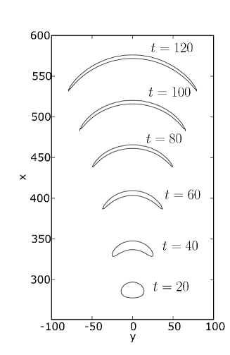
Figure 1: Stages of evolution of the space charge layer surrounding a streamer in a homogeneous background electric field of $E_{0}=1$ pointing downwards. Plotted is the half maximum line of the negative space charge density $\sigma-\rho$ at each instance of time. Similar plots in 3 spatial dimensions with radial symmetry were presented and discussed in CaroAva ; CaroJCP , the present simulation is purely 2 dimensional.

In the moving boundary approximation presented in loza73 ; Bern1 ; PRL05 ; SIAM06 the space charge layer is replaced by an infinitesimally thin interface. It is assumed that the streamer moves into a non-ionized and electrically neutral medium, so that outside the steamer the electric potential $\varphi$ obeys the Laplace equation

$$\Delta\varphi=0\qquad\quad\text{outside the streamer}.$$ (1)

The ionized body of the streamer is modeled as ideally conducting

$$\varphi=\text{const}\ \qquad\text{inside the streamer}.$$ (2)

We immediately note that this latter assumption will not be essential for our analysis. The interface separating these two regions moves with a velocity $v_{n}$ that depends on the local electric field

$$v_{n}=v^{*}\Big{(}\nabla\varphi\Big{)}^{+}.$$ (3)

Here and below, superscripts ^± indicate the limit value on the interface where the interface is approached from the outside or the inside, respectively.

In earlier work loza73 ; Bern1 , the electric potential was taken as continuous on the streamer boundary, $\varphi^{+}=\varphi^{-}$, which for an ideally conducting streamer interior implies that the moving interface is equipotential, $\varphi^{+}=\text{const}$. However, due to the small but finite width of the physical space charge layer this assumption is unfounded. Rather in moving boundary approximation $\varphi$ must be discontinuous at the interface. In PRL05 ; SIAM06 we modeled the potential difference across the interface as

$$\varphi^{+}-\varphi^{-}=\ell\,\hat{{\bf n}}\cdot(\nabla\varphi)^{+},$$ (4)

where the length parameter $\ell$ accounts for the thickness of the ionization front and $\hat{{\bf n}}$ is the exterior normal on the interface. Derivation and discussion of this boundary condition is the subject of the present paper. In the context of crystal growth from undercooled melts such a boundary condition is known as kinetic undercooling.

Clearly the model (1)–(4) is intimately related to moving boundary models for a variety of different physical phenomena like viscous fingering (see, e.g., R3 ; R4 ) or crystal growth (see, e.g., Saito ; Pom ). To derive the model in the context of streamer motion, our starting point is the minimal streamer model that applies to anode-directed discharges in simple gases like nitrogen or argon. Cathode-directed discharges or discharges in composite gases like air involve additional physical mechanisms Raizer .

In Sec. II.1 of the present paper we describe briefly the minimal streamer model. If diffusion is neglected the model allows for planar shock fronts moving with constant velocity in an externally applied, time independent electric field, and some properties of these solutions are recalled in Sec. II.2. Based on these results, in Sec. III.1, supplemented by the appendix, we present a rigorous derivation of the boundary condition (4), valid for planar fronts in strong electric fields. The relation of our model to other moving boundary models is briefly discussed in Sec. III.2. The crucial question whether the model also applies to curved ionization fronts in weaker external fields is considered in Sec. IV. Based on numerical solutions of the minimal model in two-dimensional space we argue that our moving boundary model indeed captures the essential physics of fully developed (negative) streamer fronts. Our conclusions are summarized in Sec. V.

II Collection of some previous results

II.1 The minimal streamer model

The model for negative streamers in simple non-attaching gases like nitrogen and argon as used in dhal87 ; vite94 ; PRLUWC ; CaroRapid ; CaroJCP consists of a set of three coupled partial differential equations for the electron density $\sigma$, the ion density $\rho$ and the electric field ${\bf E}$. In dimensionless units, it reads

$$\partial_{t}\sigma+\nabla\cdot{\bf j}_{e} = |\sigma{\bf E}|\;\alpha(|{\bf E}|),$$ (5)

$$\partial_{t}\rho = |\sigma{\bf E}|\;\alpha(|{\bf E}|),$$ (6)

$$\nabla\cdot{\bf E} = \rho-\sigma,\quad{\bf E}=-\nabla\varphi.$$ (7)

The first two equations are the continuity equations for the electrons and the ions while the last is the Coulomb equation for the electric field generated by the space charge $\rho-\sigma$ of electrons and ions. ${\bf j}_{e}$ is the electron particle current which we here take as the drift current only

$${\bf j}_{e}=-\sigma{\bf E}.$$ (8)

(For the effect of a diffusive contribution to the current, see a recent summary in section 2 of gianne and Sec. IV of the present paper.) The current of the much heavier ions is neglected. $|\sigma{\bf E}|\;\alpha(|{\bf E}|)$ is the generation rate of additional electron ion pairs; it is the product of the absolute value of the current $|\sigma{\bf E}|$ times the effective cross section $\alpha(|{\bf E}|)$ which is taken as field dependent; an old and much used form for $\alpha(|{\bf E}|)$ is the Townsend approximation

$$\alpha(|{\bf E}|)=e^{-1/|{\bf E}|},$$ (9)

but our analysis holds for the more general case of

$$\alpha(0) = 0,\quad\frac{d\alpha(|{\bf E}|)}{d{|{\bf E}|}}\geq 0,$$

$$\alpha(|{\bf E}|) \underset{|{\bf E}|\gg 1}{=} 1-{\cal O}\left(\frac{1}{|{\bf E}|}\right).$$ (10)

The dimensional analysis reducing the physical equations to the dimensionless model defined above can be found in many previous papers, e.g., in PRLUWC ; PSST ; PREUWC . We only note that the intrinsic time and length scales are defined in terms of the electron mobility and the effective ionization cross section and thus are determined by the physics on microscopic scales.

II.2 Planar ionization fronts

We here recall essential properties of planar negative ionization fronts as derived in PREUWC ; Man04 . We consider ionization fronts propagating in the positive $x$ direction into a medium that is completely non-ionized beyond a certain point $x_{f}(t)$

$$\sigma=0=\rho \quad\text{for}\quad x>x_{f}(t),$$ (11)

$$\sigma>0 \quad\text{for}\quad x<x_{f}(t).$$

Far ahead the front, the electric field is taken to approach a constant value:

$${\bf E}\underset{x\rightarrow+\infty}{\longrightarrow}-E_{0}\;{\hat{\bf x}},~{}~{}~{}E_{0}>0,$$ (12)

where ${\hat{\bf x}}$ is the unit vector in the $x$-direction. For a planar front, ${\bf E}$ evidently can depend only on $x$ and $t$, and Eqs. (7), (12) yield a constant field in the non-ionized region

$${\bf E}=-E_{0}\;{\hat{\bf x}},\quad x\geq x_{f}.$$ (13)

The planar solution of the model takes the form of a uniformly translating shock front moving with velocity

$$v=\partial_{t}x_{f}=-E\big{|}_{x=x_{f}}=E_{0}.$$ (14)

In the comoving coordinate

$$\xi=x-x_{f}(0)-vt,$$ (15)

a discontinuity of the electron density is located at $\xi=0$, while the ion density $\rho$ and the electric field $E$ are continuous.

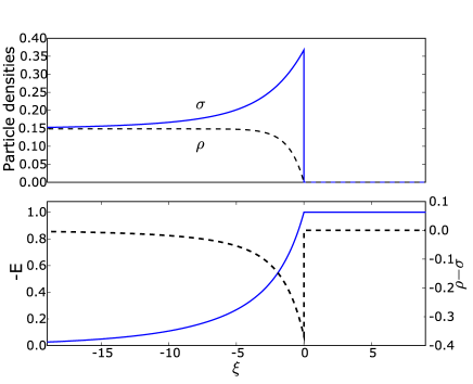
Figure 2: Densities and field in a planar ionization front in a far field $E_{0}=1$ as a function of the comoving coordinate $\xi$ (15). The front moves to the right with velocity $v=E_{0}$. Upper panel: electron density $\sigma$ (solid line) and ion density $\rho$ (dashed line); lower panel: electric field (solid line, axis on the left) and space charge density $\rho-\sigma$ (dashed line, axis on the right). For $\alpha(|{\bf E}|)$ the Townsend approximation (9) was used.

Fig. 2 that similarly has appeared in Man04 , illustrates the spatial profiles in such a uniformly translating front for $E_{0}=1$. In the non-ionized region $\xi>0$, we simply have $\rho=0=\sigma$ and $E=-E_{0}$. In the ionized region $\xi<0$, the propagating electron front creates additional electrons and ions as long as $\alpha(E)>0$, therefore the density of immobile ions $\rho$ increases monotonically behind the front. The electrons move such as to screen the conducting interior from the applied electric field. They form a layer of nonvanishing space charge $\rho-\sigma$ that suppresses the field $E$ behind the front.

Analytically the solution in the ionized region $\xi<0$ is given implicitly by the equations

$$\sigma(E) = \frac{E_{0}}{E_{0}-|E|}\;\rho(E),$$ (16)

$$\rho(E) = \int_{|E|}^{E_{0}}\alpha(\eta)\,d\eta,$$ (17)

$$-\xi = \int_{E(\xi)}^{-E_{0}}\frac{E_{0}+\eta}{\rho(\eta)}\,\frac{d\eta}{\eta}.$$ (18)

In the limit $E_{0}\gg 1$, these equations will be further evaluated below. We note that at the shock front, the electron density jumps from zero to

$$\sigma=E_{0}\,\alpha(E_{0}),$$ (19)

and for $\xi\rightarrow-\infty$ it approaches the value

$$\sigma(-\infty)=\int_{0}^{E_{0}}\alpha(\eta)\,d\eta.$$ (20)

Far behind the front, where ${\bf E}$ is so small that $\alpha(|{\bf E}|)\simeq 0$, the final relaxation of E and of $\sigma$ is exponential in space: $\sim e^{-\lambda\xi}$, where

$$\lambda=\frac{\sigma(-\infty)}{v}=\frac{1}{E_{0}}\int_{0}^{E_{0}}\alpha(\eta)\,d\eta\stackrel{{\scriptstyle E_{0}\to\infty}}{{\longrightarrow}}1.$$ (21)

III The moving boundary model

III.1 Construction

The results reviewed in the previous section (see also Fig. 1) show that a layer of space charge $\rho-\sigma$ screens the electric field from the streamer interior. For strong applied electric field $-E_{0}$, the thickness of this layer defines some small inner scale of the front, while on the large outer scale, the streamer will be approximated as a sharp interface separating an ionized but electrically neutral region inside the streamer from the non-ionized charge free region outside the streamer; this substantiates the assumptions underlying the moving boundary model treated in PRL05 ; SIAM06 .

Being a shock front solution of Eq. (5), the interface always moves with normal velocity

$$v_{n}=\hat{{\bf n}}\cdot(\nabla\varphi)^{+},$$ (22)

where $\hat{{\bf n}}$ is the unit vector normal to the interface pointing into the exterior region; this equation generalizes Eq. (14). We recall that ⁺ indicates that the expression is evaluated by approaching the interface from outside the streamer.

As mentioned in the introduction, in the context of electric breakdown the moving boundary model (1), (2), (22) has been formulated some time ago by Lozansky and Firsov loza73 . To complete the model, a boundary condition at the interface is needed, and in Ref. loza73 continuity of the potential at the interface was postulated:

$$\varphi^{+}=\varphi^{-}=\text{const}.$$ (23)

However, Fig. 2 clearly shows that crossing the screening layer, $\varphi(\xi)$ will increase, which amounts to a jump $\varphi^{+}>\varphi^{-}$ in the interface model. The size of this jump depends on the electric field ${\bf E}^{+}$ at the interface and for a planar front is easily determined from Eq. (18). We note that in the framework of the PDE-model, (Sec. II), $\varphi^{\pm}$ are to be identified as

$$\varphi^{-}=\varphi(-\infty),\quad\varphi^{+}=\varphi(0),$$ (24)

$$\varphi^{+}-\varphi^{-}=-\int_{-\infty}^{0}E\,d\xi.$$ (25)

Since $E(\xi)$ according to (17), (18) is a monotonically decreasing function for $\xi<0$, we can integrate by parts

$$\varphi^{+}-\varphi^{-} = -\int_{-\infty}^{0}E\,d\xi=(\xi E)\Big{|}_{-\infty}^{0}+\int_{0}^{E^{+}}\xi\,dE$$ (26)

$$= \int_{0}^{E^{+}}\xi\,dE.$$

The last identity holds since either $E$ or $\xi$ vanish on the integration boundaries. For a planar front, we have $E^{+}=-E_{0}$, but we here keep $E^{+}$ to stress the dependence on the field at the front position $\xi=0$.

While $E(\xi)$ is known only implicitly as $\xi=\xi(E)$ in Eq. (18), the partial integration now allows us to evaluate the integral explicitly by substituting Eq. (18) in (26):

$$\varphi^{+}-\varphi^{-} = -\int_{0}^{E^{+}}dE\int_{E}^{E^{+}}\frac{\eta-E^{+}}{\rho(\eta)}\;\frac{d\eta}{\eta}$$ (27)

$$= -\int_{0}^{E^{+}}\frac{\eta-E^{+}}{\rho(\eta)}\,d\eta.$$ (28)

$\rho(\eta)$ is given in Eq. (17). This result explicitly shows that in the interface model the potential is discontinuous across the boundary, where the size of the discontinuity depends on the electric field right ahead of the ionization front.

Evaluating Eq. (28), in the appendix we derive bounds showing that $\varphi^{+}-\varphi^{-}\approx-E^{+}+\text{ const}$ for large $|E^{+}|$. We here present a simpler argument yielding only the leading term. It is based on direct evaluation of Eqs. (17), (18), written as

$$\frac{\rho(E)}{|E^{+}|} = \int_{\frac{E}{E^{+}}}^{1}\alpha\left(\eta\,|E^{+}|\right)d\eta$$ (29)

$$\xi = |E^{+}|\int_{\frac{E(\xi)}{E^{+}}}^{1}\frac{\nu-1}{\rho(\nu E^{+})}\frac{d\nu}{\nu}.$$ (30)

We now take the limit $|E^{+}|\to\infty$ in Eq. (29), with $E/E^{+}>0$ fixed. The asymptotic behavior (II.1) of $\alpha(|{\bf E}|)$ yields

$$\frac{\rho(E)}{|E^{+}|}=1-\frac{E}{E^{+}}.$$ (31)

Substituting this result into Eq. (30) we find

$$\xi=-\int_{E(\xi)/{E}^{+}}^{1}\frac{d\nu}{\nu},$$

yielding a purely exponential front profile

$$E(\xi)=E^{+}e^{\xi}.$$ (32)

This result means that the exponential decay of the space charge layer (21), that holds far behind the front for all $|E^{+}|>0$, for $|E^{+}|\gg 1$ is actually valid throughout the complete front up to $\xi=0$. Substituting Eq. (32) into Eq. (25), we find $\varphi^{+}-\varphi^{-}=-E^{+}$.

The more precise argument given in the appendix shows that $(\varphi^{+}-\varphi^{-})/|E^{+}|$ decreases monotonically with $|E^{+}|$ and is bounded as

$$0 \leq \frac{\varphi^{+}-\varphi^{-}}{|{E}^{+}|}-1$$

$$\leq \frac{2\,b}{|E^{+}|}+{\cal O}\left(\left({\frac{b}{|E^{+}|}}\right)^{2}\ln\left(\frac{|E^{+}|}{b}\right)\right)\mbox{ for }|{\bf E}^{+}|\to\infty,$$

where $b>0$ is some constant. The result

$$\varphi^{+}-\varphi^{-}=-E^{+}+b^{\prime}+{\cal O}\left(\frac{\ln|E^{+}|}{E^{+}}\right)$$ (34)

follows. It shows that the first correction to the leading behavior $\varphi^{+}-\varphi^{-}\sim-E^{+}$ is just a constant, not a logarithmic term. We thus can choose the gauge of $\varphi$ as $\varphi^{-}+b^{\prime}=0$ to find $\varphi^{+}=-E^{+}+{\cal O}(\ln|E^{+}|/E^{+})$.

The simplest generalization of this result to curved fronts in strong fields, $|E^{+}|\gg 1$, suggests the boundary condition

$$\varphi^{+}=\hat{{\bf n}}\cdot(\nabla\varphi)^{+},$$ (35)

replacing the Lozansky-Firsov boundary condition (23). Boundary condition (35) together with the Laplace equation $\Delta\varphi=0$ (1) and the interfacial velocity ${\bf v}=\nabla\varphi$ (22) define our version of the moving boundary model describing the region outside the streamer and the consecutive motion of its boundary.

III.2 Discussion

The model formulated here belongs to a class of Laplacian moving boundary models describing a variety of phenomena. In particular, it is intimately related to the extensively studied models of viscous fingering R3 ; R4 and solidification in undercooled melts Saito ; Pom . In all these models the boundary separates an interior region from an exterior region, where the relevant field obeys either the Laplace equation or a diffusion equation, and the velocity of the interface is determined by the gradient of this field.

If we replace the boundary condition (35) by (23): $\varphi^{+}=\text{const.}$, the model becomes equivalent to a simple model of viscous fingering where surface tension effects are neglected. This “unregularized” model is known to exhibit unphysical cusps within finite time R2 ; R1 . To suppress these cusps, in viscous fingering a boundary condition involving the curvature of the interface is used. The physical mechanism for this boundary condition is surface tension. As mentioned in the introduction, the kinetic undercooling boundary condition (35) is used in the context of solidification. In that case, however, the relevant temperature field obeys the diffusion equation. From a purely mathematical point of view, our model with specific conditions on the outer boundaries far away from the moving interface has been analyzed in R6 ; R5 ; R9 . It has been shown R9 that with outer boundary conditions appropriate for Hele-Shaw cells, the kinetic undercooling condition selects the same stable Saffman-Taylor finger configuration as curvature regularization. Furthermore it has been proven R6 ; R5 that an initially smooth interface stays smooth for some finite time. This regularizing property of the boundary condition (35) is also supported by our previous and ongoing work PRL05 ; SIAM06 ; R10 .

In applying an interface model to streamer propagation, an important difference from the other physical systems mentioned above must be noted. For the other systems mentioned the moving boundary model directly results from the macroscopic physics, irrespective of the motion of the boundary: a sharp interface with no internal structure a priori is present. In contrast, a streamer emerges from a smooth seed of electron density placed in a strong electric field, and the screening layer that is an essential ingredient of the moving boundary model, arises dynamically, with properties determined by the electric field and thus coupled to the velocity of the boundary. The model therefore does not cover the initial “Townsend” or avalanche stage of an electric discharge CaroAva that is also visible in Fig. 1, but can only be applied to fully developed negative streamers. Furthermore, being explicitly derived for planar fronts, the validity of the boundary condition for more realistic curved streamer fronts has to be tested. This issue is discussed in the next section.

IV Curved streamer fronts in two dimensions

IV.1 Illustration of numerical results for fully developed streamers

We solve the PDE-model (5)-(7) in two dimensions, using the numerical code described in detail in CaroJCP . (Previous simulation work was in three spatial dimensions assuming radial symmetry of the streamer, the results are very similar.) In the electron current ${\bf j}_{e}$, besides the drift term $-\sigma\,{\bf E}$, a diffusive contribution is taken into account:

$${\bf j}_{e}=-\sigma{\bf E}-D\nabla\sigma.$$ (36)

This clearly is adequate physically, and on the technical level it smoothes the discontinuous shock front. The price to be paid is some ambiguity in defining the position of the moving boundary, see below.

Planar fronts with $D>0$ have been analyzed in PRLUWC ; PREUWC ; gianne , for further discussion and illustrations, we refer to section 2 of gianne . It is found that diffusion enhances the front velocity by a term

$$v_{n,D}=2\sqrt{D|E^{+}|\alpha(|E^{+}|)},$$

that has to be added to the velocity $v_{n,\text{drift}}=|E^{+}|$. Furthermore, diffusion creates a leading edge of the electron density in forward direction which decreases exponentially on scale

$$\ell_{D}=\sqrt{\frac{D}{|E^{+}|\alpha(|E^{+}|)}}.$$

This scale has to be compared to the thickness of the screening layer for $D=0$: $\ell_{\alpha}\sim 1/\alpha(|{E}^{+}|)$. For large $|E^{+}|$ and small D both the ratios $v_{n,D}/v_{n,\text{drift}}$ and $\ell_{D}/\ell_{\alpha}$ are of order $\sqrt{D/|E^{+}|}\ll 1$. This, by itself, does not imply that diffusion can be neglected since the term $D\nabla\sigma$ is a singular perturbation of the diffusion free model. However, in our numerical solutions the main effect of diffusion is found to amount to some rescaling of the parameters in the effective moving boundary model, see below. This is consistent with the observation that for long wave length perturbations of planar fronts, the limit $D\to 0$ is smooth gianne .

In our numerical calculations, we take $D=0.1$. For $\alpha(|{\bf E}|)$ the Townsend form (9) is used. We start with an electrically neutral, Gaussian shaped ionization seed, placed in a constant external electric field ${\bf E}=-E_{0}\,\hat{{\bf x}}$. We performed runs for $0.5\leq E_{0}\leq 2$. Since the thickness of the screening layer decreases with increasing $E_{0}$, higher fields need better numerical resolution, enhancing the numerical cost considerably. In view of the results shown below we do not expect qualitative changes for $E_{0}>2$.

The system (5)–(7) is solved numerically with a spatial discretization of finite differences in adaptively refined grids and a second-order explicit Runge-Kutta time integration, as described in detail in CaroJCP , with the difference that the method described there was for three dimensional streamers with cylindrical symmetry and here we adapted it to truly two-dimensional systems. The highest spatial resolution in the area around the streamer head was $\Delta x=\Delta y=1/4$ for all simulations.

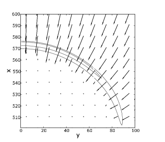
Figure 3: Zoom into the right half of the symmetric streamer head at time step $t=120$ of Fig. 1 in a background field of $E_{0}=1$. Shown are level lines of negative space charge density $\sigma-\rho$ (at levels 1/3 and 2/3 of the maximal density) and arrows indicating the local electric field at the foot point of the arrow.

For external field $E_{0}=1$, Fig. 1 illustrates the temporal evolution of the streamer head. We see that initially, a screening layer forms out of an ionization avalanche, this process is discussed in detail in CaroAva . The width of the layer rapidly reaches some almost constant value that depends on $E_{0}$. The head develops into a somewhat flattened semicircle, with the radius increasing with time. This stage of evolution will be addressed as the fully developed streamer. Fig. 3 zooms into the streamer head at this stage, showing lines of constant charge density $\rho-\sigma$ together with electric field vectors. Evidently screening is not complete. A small, essentially constant field exists behind the streamer head. This is illustrated in Fig. 4 that shows the variation of the electric field and of the excess charge along the symmetry line $y=0$. This figure shows also that the spatial positions of the maxima of $|{\bf E}|$ and of $\sigma-\rho$ do not coincide precisely; in fact, the maximum of $|{\bf E}|$ lies within the diffusive leading edge of the front; the small width $\ell_{D}$ of this diffusive layer replaces the jump of the electron density for $D=0$. We furthermore observe that the field behind the front is suppressed by about a factor of $1/20$ compared to the maximal value $|{\bf E}|\approx 2.1$, or equivalently to $\approx\!E_{0}/10$. This screening increases with increasing background electric field $E_{0}$: from $\approx\!E_{0}/7$ for $E_{0}=0.5$ to $\approx\!E_{0}/20$ for $E_{0}=2.0$. (The maximal field enhancement in these cases is $\gtrsim 2\;E_{0}$ in the fully developed streamer briefly before branching.)

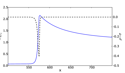
Figure 4: The same case as in Fig. 3, plotted is now the negative electric field (solid line, axis on the left) and the space charge density (dashed line, axis on the right) on the axis of the streamer. The plot can be compared to the lower panel in Fig. 2 showing a planar front with vanishing diffusion.

IV.2 Test of the assumptions of the moving boundary model

The moving boundary model is concerned only with the exterior region. Recalling the defining equations

$$\Delta\varphi = 0,\qquad\quad\text{in exterior region},$$ (37)

$$v_{n} = -\hat{{\bf n}}\cdot{\bf E}^{+},$$ (38)

$$\varphi^{+} = -\hat{{\bf n}}\cdot{\bf E}^{+},$$ (39)

we note that all explicit reference to the physics in the interior is absent, notwithstanding our derivation in Sec. III. Now the first of these equations evidently holds as soon as the diffusive leading edge of the electron density has a negligible space charge density. Also the second relation holds for any smooth shock front ($D=0$) of the PDE-model. The boundary condition (39), however was derived only for planar fronts in strong external fields $E_{0}\gg 1$.

To check whether the moving boundary model adequately represents the evolution of curved streamer fronts for small diffusion and external fields of order unity, we first have to choose a precise definition of the interface. As illustrated in Figs. 3 and 4, the screening layer is fairly thin, but nevertheless it involves the two length scales $\ell_{D}$ and $\ell_{\alpha}$ and thus shows some intrinsic structure. We define the moving boundary to be determined by the maximum of $|{\bf E}(x,y)|$ along intersections perpendicular to the boundary. In precise mathematical terms a parameter representation ($x_{b}(u),y_{b}(u)$) of the boundary obeys the equation

$$0=\hat{{\bf n}}(u)\cdot\nabla|{\bf E}||_{x=x_{b}(u),y=y_{b}(u)},$$

where

$$\hat{{\bf n}}(u)\sim\left(\frac{dy_{b}}{du},-\frac{dx_{b}}{du}\right)$$

is the normal to the boundary at point $(x_{b}(u),y_{b}(u))$. To motivate this choice we note that the moving boundary model explicitly refers only to ${\bf E}$ and not to the excess charge distribution. In practice we determine ($x_{b}(u),y_{b}(u)$) by first searching for the maxima of $|{\bf E}|$ along horizontal or vertical intersections, and we then iteratively refine the so determined zero order approximation. We always follow the boundary up to the point where the local value of $|{\bf E}^{+}|$ equals $E_{0}$. This covers all the head of the streamer, where the essential physics takes place. Fig. 5 shows the resulting boundary corresponding to the snapshot of Fig. 3. We observe that the direction of ${\bf E}$ is close to, but does not precisely coincide with the normal direction on the interface (except on the symmetry axis, of course). The boundary is not equipotential but a small component of the electric field tangential to the boundary drives the electrons toward the tip. This effect counteracts the stretching of the space charge layer perpendicular to the direction of streamer motion, (see Fig. 1), which in itself would lead to a weakening of screening.

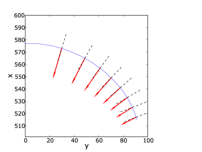
Figure 5: Again the situation of Figs. 3 and 4. Shown is now the boundary defined by the maximum of $E$ on normal intersections (solid line), the local directions of the surface normal (dashed lines) and the local electric fields (solid arrows).

With the so defined interface we have checked that $v_{n}$ depends linearly on $E^{+}$ within the numerical precision, therefore Eq. (38) holds, except for an increase of the ratio $v_{n}/|\hat{{\bf n}}\cdot{\bf E}^{+}|$, which is an expected effect of diffusion PRLUWC ; PREUWC ; gianne ; this effect can be absorbed into a rescaling of time.

The essential test of the boundary condition (39) is shown in Fig. 6. It shows how $\varphi^{+}$ depends on $|\hat{{\bf n}}\cdot{\bf E}^{+}|$ along the boundary for several values of $E_{0}$ measured at times where the streamer is fully developed. For each set of data we first determine $\varphi^{+}$ at the maximum of $E^{+}$, i.e. at $y=0$. This constant $\varphi^{+}(E_{max}^{+})$ is subtracted from all values $\varphi^{+}$ along the interface. Except for the smallest external field $E_{0}=0.5$, the plots in Fig. 6 clearly are linear within the scatter of the data. Even for $E_{0}=0.5$ the curvature is very small. (We note that with increasing $E_{0}$, the width $\ell_{D}$ of the diffusion layer decreases and approaches the limiting spatial resolution of the numerics CaroJCP . This explains the increasing scatter of the data with increasing $E_{0}$). Furthermore, as is illustrated in Fig. 7 for $E_{0}=1.0$, for a fixed $E_{0}$ the slope of the relation between $\varphi^{+}$ and $|\hat{{\bf n}}\cdot{\bf E}^{+}|$ does not depend on time. Thus these numerical results can be summarized by the relation

$$\varphi^{+}=\varphi_{0}(E_{0},t)-\ell(E_{0})\,\hat{{\bf n}}\cdot{\bf E}^{+}.$$ (40)

Of course, neither the PDE-model nor the moving boundary approximation depend on the gauge $\varphi_{0}(E_{0},t)$ which thus can be ignored. The prefactor $\ell(E_{0})$ can be absorbed into the length scale of the moving boundary model, with a compensating change of the time scale to preserve Eq. (38). As mentioned above, this rescaling also can absorb the enhancement of $v_{n}$ due to diffusion. As a result, the model (37)-(39) adequately appears to describe also fully developed curved streamer fronts.

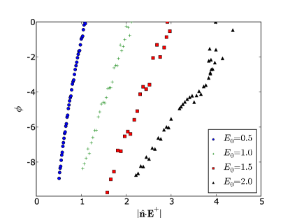
Figure 6: $\varphi^{+}$ as a function of $E^{+}$ along the interface for different background fields $E_{0}$. A gauge constant $\varphi^{+}(E_{max}^{+})$ is subtracted from $\varphi^{+}$ for each data set. For each electric field, the data was extracted at times long enough for the space charge layer to be fully developed, but always before the streamer branches. These times were $t=500$ for $E_{0}=0.5$, $t=120$ for $E_{0}=1.0$, $t=43.6$ for $E_{0}=1.5$ and $t=35$ for $E_{0}=2.0$.

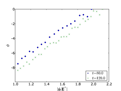
Figure 7: $\varphi^{+}$ as a function of $E^{+}$ in a background field $E_{0}=1$ for times $t=80$ and $120$. The slope is the same.

We finally note that the parameter $\ell(E_{0})$ decreases with increasing $E_{0}$, and it is well conceivable that for $E_{0}\rightarrow\infty$ it tends to $1$, as predicted by our analysis of planar fronts. Furthermore this behavior parallels the behavior of the thickness of the screening layer, suggesting the very plausible assumption that it is this thickness which sets the spatial scale of the model also away from the limit $E_{0}\rightarrow\infty$.

V Conclusions

Starting from a PDE-model of an anode-directed streamer ionization front, we have derived a boundary condition valid for a moving boundary model of the streamer stage of the discharge. Due to the finite width of the space charge layer surrounding the streamer head, in a moving boundary approximation the electric potential has to be discontinuous across the boundary, and the boundary condition (39) proposed here accounts for this jump in a very simple way. Our analytical derivation is restricted to planar fronts in extreme external fields $E_{0}\rightarrow\infty$, but the analysis of numerical solutions of the PDE-model shows that the boundary condition also applies to (two-dimensional) curved ionization fronts in weaker external fields. We conclude that the moving boundary model adequately represents the evolution of negative streamer fronts. This conclusion can also be drawn from studies of periodic arrays of interacting streamers that show strong similarities with Saffman-Taylor fingers and will be presented elsewhere R11 .

As with other moving boundary models in two dimensions, we now are in a position to use powerful conformal mapping techniques to analytically attack questions like the stability of streamers against branching. Some first results can be found in Refs. PRL05 ; SIAM06 .

The moving boundary model does not explicitly refer to the interior of the streamer and thus leaves open questions concerning the role of the residual electric field and the resulting currents inside the streamer. Analyzing such questions within the framework of the minimal PDE model should lead to a more detailed understanding of the structure of the space charge layer for curved fronts and should clarify the physics underlying the phenomenological length parameter $\ell(E_{0})$ occurring in Eq. (40). This problem, which is important for fully understanding the physics of the streamer, is left for future work.

Acknowledgement: F.B. and A.L. were both supported by the Netherlands Organization for Scientific Research NWO, F.B. through project 633.000.401 within the program ”Dynamics of Patterns”, and A.L. by the Foundation for Technological Sciences STW, project CTF.6501. B.M. acknowledges a Ph.D. grant from CWI.

Appendix A Bounds on $\varphi^{+}-\varphi^{-}$

Basic for our discussions are the properties of $\alpha(\eta)$ quoted in Eq. (II.1), valid for $\eta\geq 0$:

$$0\leq\alpha(\eta)\leq 1,\quad\lim_{\eta\rightarrow\infty}\alpha(\eta)=1,$$ (41)

$$\frac{d\alpha}{d\eta}\geq 0.$$ (42)

We furthermore add the physically reasonable condition that

$$0<b=\sup_{\eta\geq 0}\left(-\frac{d\alpha(1/\eta)}{d\eta}\right)<\infty$$ (43)

exists, so that $\alpha(\eta)$ obeys the bound

$$\alpha(\eta)\geq 1-\frac{b}{\eta}.$$ (44)

We now rewrite Eq. (17) for $\rho(E)$ as

$$\rho(E)=(|E^{+}|-|E|)\;\bar{\rho}\left(\frac{E}{E^{+}},|E^{+}|\right),$$ (45)

where

$$\bar{\rho}(z,|E^{+}|)=\int_{0}^{1}\alpha\left(|E^{+}|\left(z+(1-z)y\right)\right)\,dy.$$ (46)

Eq. (28) for $\varphi^{+}-\varphi^{-}$ takes the form

$$\frac{\varphi^{+}-\varphi^{-}}{|E^{+}|}=\int_{0}^{1}\frac{dx}{\bar{\rho}(x,|E^{+}|)}.$$ (47)

The assumption (41) that $\alpha(E)\leq 1$ for all $E$, leads directly to the lower bound

$$\frac{\varphi^{+}-\varphi^{-}}{|E^{+}|}\geq 1.$$ (48)

We note that a better lower bound can be obtain from the fact that since $\alpha\left(E^{+}\left(x(1-y)+y\right)\right)$ increases with $x$, the function $\bar{\rho}(x,E^{+})$ obeys

$$\bar{\rho}(x,|E^{+}|)\leq\alpha(|E^{+}|).$$

This leads to the improved lower bound

$$\varphi^{+}-\varphi^{-}\geq\frac{|E^{+}|}{\alpha(|E^{+}|)},$$ (49)

illustrating that weak fields cannot be screened since $|E^{+}|/\alpha(|E^{+}|)$ typically diverges for $|E^{+}|\rightarrow 0$.

To derive an upper bound valid for large fields, we assume $|E^{+}|>b$ and split the integral in Eq. (47) as

$$\int_{0}^{1}\frac{dx}{\bar{\rho}(x,|E^{+}|)}=I_{1}+I_{2},$$ (50)

where

$$I_{1} = \int_{0}^{b/|E^{+}|}\frac{dx}{\bar{\rho}(x,|E^{+}|)},$$ (51)

$$I_{2} = \int_{b/|E^{+}|}^{1}\frac{dx}{\bar{\rho}(x,|E^{+}|)}.$$ (52)

By virtue of Eq. (42), $\bar{\rho}(x,|E^{+}|)$ increases with $x$, which immediately yields the bound

$$I_{1}\leq\frac{b}{|E^{+}|}\bar{\rho}(0,|E^{+}|)^{-1}.$$

Evaluating $\bar{\rho}(0,|E^{+}|)$ with the bound (44) on $\alpha(\eta)$ yields

$$I_{1}\leq\frac{b}{|E^{+}|}\left[1-\frac{b}{|E^{+}|}\left(1+\ln(|E^{+}|/b)\right)\right]^{-1}.$$ (53)

To evaluate $I_{2}$ we write

$$\bar{\rho}(x,|E^{+}|) = \int_{0}^{x}\alpha(|E^{+}|(x+(1-x)y))\,dy$$

$$+ \int_{x}^{1}\alpha(|E^{+}|(y+(1-y)x))\,dy$$

$$> \int_{0}^{x}\alpha(|E^{+}|x)\,dy+\int_{x}^{1}\alpha(|E^{+}|y)\,dy,$$

$$> 1-\frac{b}{|E^{+}|}+\frac{b}{|E^{+}|}\ln x.$$

This result yields

$$I_{2} < 1-\frac{b/|E^{+}|}{1-b/|E^{+}|}\int_{b/|E^{+}|}^{1}\frac{\ln x}{1-b(1-\ln x)/|E^{+}|}\,dx,$$ (54)

$$< 1-\frac{b/|E^{+}|}{1-b/|E^{+}|}\times$$

$$\times \frac{1}{1-b(1-\ln(b/|E^{+}|))/|E^{+}|}\int_{b/|E^{+}|}^{1}\ln x\,dx,$$

$$= \frac{1}{1-b/|E^{+}|}.$$

Collecting all the results (and recalling $b/|E^{+}|<1$), we found in this appendix that

$$\frac{\varphi^{+}-\varphi^{-}}{|E^{+}|}<\frac{1}{1-b/|E^{+}|}+\frac{b/|E^{+}|}{1-\frac{b}{|E^{+}|}\left(1+\ln(|E^{+}|/b)\right)},$$ (55)

which for large $|E^{+}|/b$ leads to the bound (III.1) given in the main text. We note, in particular, that $\varphi^{+}-\varphi^{-}$ does not contain a contribution of order $\ln(|E^{+}|/b)$, so that the leading (constant), correction to $\varphi^{+}-\varphi^{-}=-E^{+}$ can be gauged away.

We finally note that Eqs. (46), (42) imply that $\bar{\rho}(x,|E^{+}|)$ increases monotonically with $|E^{+}|$, and thus that $(\varphi^{+}-\varphi^{-})/|E^{+}|$ decreases monotonically.

References

- (1) H. Raether, Z. Phys. 112, 464 (1939).
- (2) L.B. Loeb and J.M. Meek The Mechanism of the Electric Spark (Stanford, CA: Stanford Univ. Press, 1941).
- (3) Yu.P. Raizer, Gas Discharge Physics (Berlin: Springer, 1991).
- (4) U. Ebert et al., Plasma Sources Sci. Technol. 15, S118 (2006).
- (5) C. Wu and E.E. Kunhardt, Phys. Rev. A 37, 4396 (1988).
- (6) S. K. Dhali and P. F. Williams, Phys. Rev. A 31, 1219 (1985).
- (7) S. K. Dhali and P. F. Williams, J. Appl. Phys. 62, 4696 (1987).
- (8) P. A. Vitello, B. M. Penetrante, and J. N. Bardsley, Phys. Rev. E 49, 5574 (1994).
- (9) M. Arrayás, U. Ebert and W. Hundsdorfer, Phys. Rev. Lett. 88, 174502 (2002).
- (10) A. Rocco, U. Ebert and W. Hundsdorfer, Phys. Rev. E 66, 035102(R) (2002).
- (11) C. Montijn, U. Ebert, J. Phys. D: Appl. Phys. 39, 2979 (2006).
- (12) C. Montijn, U. Ebert and W. Hundsdorfer, Phys. Rev. E 73, 065401 (2006).
- (13) C. Montijn, W. Hundsdorfer and U. Ebert, J. Comp. Phys. 219, 801 (2006).
- (14) E. D. Lozansky and O. B. Firsov, J. Phys. D: Appl. Phys. 6, 976 (1973).
- (15) U. Ebert, W. van Saarloos and C. Caroli, Phys. Rev. Lett. 77, 4178 (1996).
- (16) U. Ebert, W. van Saarloos and C. Caroli, Phys. Rev. E 55, 1530 (1997).
- (17) B. Meulenbroek, A. Rocco and U. Ebert, Phys. Rev. E 69, 067402 (2004).
- (18) B. Meulenbroek, U. Ebert and L. Schäfer, Phys. Rev. Lett. 95, 195004 (2005).
- (19) U. Ebert, B. Meulenbroek and L. Schäfer, arXiv:nlin.PS/0606048.
- (20) P.G. Saffman, G.I. Taylor, Proc. R. Soc. A 245, 317 (1958).
- (21) D. Bensimon, L.P. Kadanoff, S. Liang, B.I. Shraiman, and C. Tang, Rev. Mod. Phys. 58, 977 (1986).
- (22) Y. Saito, Statistical Physics of Crystal Growth, part IV (World Scientific, New Jersey, 1996).
- (23) Y. Pomeau and M. Ben Amar, in: Solids far from Equilibrium, edited by C. Godréche (Cambridge University Press, Cambridge 1992).
- (24) G. Derks, U. Ebert, B. Meulenbroek, arXiv:0706.2088.
- (25) M. Arrayás and U. Ebert, Phys. Rev. E 69, 036214 (2004).
- (26) B. Shraiman, D. Bensimon, Phys. Rev. A 30, 2840 (1984).
- (27) S.D. Howison, J.R. Ockendon, and A.A. Lacey, Q. Jl. Mech. appl. Math. 38, Pt3, 343 (1985).
- (28) Yu.E. Hohlov, M. Reissig, Eur. J. Appl. Math. 6, 421 (1995).
- (29) G. Prokert, Eur. J. Appl. Math. 10, 607 (1999).
- (30) S.J. Chapman, J.R. King, J. Engineering Math. 46, 1 (2003).
- (31) S. Tanveer, U. Ebert, F. Brau, L. Schäfer, [in preparation].
- (32) A. Luque, F. Brau, U. Ebert, [in preparation].