The effect of baryon cooling on the statistics of giant arcs and multiple quasars

Abstract

The statistics of giant arcs and large separation lensed quasars provide powerful constraints for the parameters of the underlying cosmological model. So far, most investigations have been carried out using pure dark matter simulations. Here we present a recipe for including the effects of baryon cooling (i.e. large galaxy formation) in dark matter $N$-body simulations that is consistent with observations of massive galaxies. Then we quantitatively compare lensing with and without applying this baryon correction to the pure dark matter case. Including the baryon correction significantly increases the frequency of giant arcs and lensed quasars, particularly on scales of 10 arcsec and smaller: the overall frequency of multiple images increases by about 25% for source redshifts between $z_{s}=1.5$ and $7.5$ and splittings larger than about 3 arcsec. The baryon rearrangement also slightly increases the fraction of quadruple images over doubles.

1 Introduction

It has been realized for some time that the abundance of clusters of galaxies can provide very stringent constraints on cosmological models (e.g. Henry & Arnaud, 1991; Oukbir & Blanchard, 1992; White, Efstathiou, & Frenk, 1993; Bahcall & Cen, 1993; Eke, Cole & Frenk, 1996; Viana & Liddle, 1996; Bahcall & Bode, 2003, and references therein). The reason for this is that— since only 5% to 10% of the stellar mass is in rich clusters, the exact fraction being fixed by the definition of “rich”— they represent relatively rare fluctuations of approximately two sigma. Consequently, as they lie on the tail of the density distribution, relatively small changes in the mean amplitude of the cosmic perturbation spectrum can produce large changes in the expected numbers of rich clusters. In fact, gravitational lensing by clusters, which depends on the most dense fraction of these systems, provides an especially sensitive measure of cosmological parameters (Turner, 1990; Wambsganss et al., 1995; Bartelmann et al., 1998; Li & Ostriker, 2002, 2003; Li et al., 2007). At the present time there is significant uncertainty in the normalization of the fluctuation power spectrum. For example, Spergel et al. (2006) give an estimate based on WMAP 3-year and SDSS data that is significantly lower than the WMAP 1-year data, but Evrard et al. (2007) argue that the cluster X-ray data indicate a higher normalization cosmology. It is hoped that efforts such as the present paper, based on ray-tracing through specific cosmological models, can help resolve this controversy.

The frequency of giant arcs and large separation quasar lenses has received increasing interest in the last few years as a powerful tool for constraining cosmological parameters. The recent discovery of a few widely separated quasar lenses ($\Delta\theta\geq 10$ arcsec) from the Sloan Digital Sky Survey (Inada et al., 2003, 2005, 2006; Oguri et al., 2004; Sharon et al., 2005) has also spurred such studies. Almost all theoretical studies using $N$-body simulations are constrained on dark matter only (Bartelmann et al., 1998; Wambsganss et al., 1995, 1998; Meneghetti et al., 2003; Wambsganss et al., 2004; Dalal, Holder & Hennawi, 2004; Oguri & Keeton, 2004; Ho & White, 2005; Horesh et al., 2005; Li et al., 2005, 2007; Hennawi et al., 2007a, b; Hilbert et al., 2007). In such studies it is usually assumed that the baryonic matter essentially follows the dark matter particles. This may be true in general on large scales, but it certainly is not a very good assumption in the central parts of galaxy clusters or for very massive isolated galaxies, which are precisely the essential matter concentrations for the production of giant arcs and wide quasar lenses. The baryonic component is also known to dominate in the central regions of elliptical galaxies.

Recent studies have begun investigating the influence of baryons on DM clustering. Puchwein et al. (2005) looked into the effect of gas physics on strong lensing by individual galaxy clusters. They found that cooling and star formation can increase the strong-lensing efficiency considerably. Jing et al. (2006) studied the influence of baryons on the clustering of matter and weak-lensing surveys, and found that the clustering of total matter is suppressed by about 1% on large scales of $1h{\rm Mpc}^{-1}\lesssim k\lesssim 10h{\rm Mpc}^{-1}$, while it is boosted between 2% and 10% on small scales of $k\approx 20h\rm{Mpc}^{-1}$; they conclude that this should be measurable with future weak lensing surveys (Jing et al. 2006). Lin et al. (2006) looked into the influence of baryons on the mass distribution of dark matter halos and found an increase of the concentration parameters by 3% to 10% as compared to pure $N$-body simulations. Rozo et al. (2006) studied the effect of baryonic cooling on giant arc abundances for individual clusters; they found that the arc abundances can be increased by factors of a few.

In this study we quantitatively investigate the effect of baryon cooling on the statistics of arcs and widely separated multiple quasars. We first motivate and describe a simple recipe for redistributing part of the matter in the centers of halos to approximate the effects of cooling and star formation, and present some tests of this method. Subsequently we summarize our use of the ray shooting method. Then we describe the quantitative results of our baryon redistribution recipe by directly comparing pseudo-three-dimensional ray shooting simulations with and without this baryon cooling, and finally discuss this effect with respect to the observational situation.

2 Methods

2.1 Baryon rearrangement

In order to approximate the effects of galaxy formation in our ray shooting simulations, we locate halos in all lens planes and identify the amount of mass likely to have cooled into stars. This mass will be rearranged such that the inner part of the total profile is isothermal. Such an approach is supported by observations, e.g. Peng et al. (2004) or Gavazzi et al. (2007), who have found that early-type galaxies are consistent with an isothermal profile out to $\geq 300$ $h^{-1}$kpc from both kinematical and lensing data. Here we describe in detail the ways this rearrangement is performed. The approach that we adopt is admittedly very rough, and so, as in all semi-analytical modeling, we constrain the free parameters to respect observational data. The requirements the model must fulfill are: a) The fraction of the baryonic component which is rearranged into stellar systems is consistent with the stellar mass fraction of the universe (cf. Figures 2 and 3). b) The cosmic buildup of mass in stellar systems parallels what is known from observations (Figure 3). c) Individual mass profiles within the baryonically dominated systems are consistent with kinematic and gravitational lensing data (Figure 4). d) The distribution of systems as a function of stellar mass and circular velocity approximates observational data (Figures 2 and 4).

Suppose we have projected the mass in some volume onto a plane for the purpose of ray tracing (as described in the next section). Let us denote the surface density of a given pixel as $\sigma$ and the pixel size as $l$, so that the mass in each pixel is $\sigma l^{2}$. For a given 2-D plane, each pixel is examined in turn to see if it has a higher surface density than any other pixel within a radius roughly the size of the smallest objects resolved in the simulation, $R_{b}=30h^{-1}$kpc physical. If so, this pixel is taken to be the center of a halo. For a given cooling radius $R_{c}$ (to be determined below), the background surface density $\sigma_{bg}$ is set to the mean surface density between $R_{c}$ and $R_{c}+(R_{b}/2)$. The mass of the halo is defined as

$$M_{h}=\int W(R/R_{c})\left[\sigma({\bf R})-\sigma_{bg}\right]dA\hskip 28.45274pt,$$ (1)

integrating from the halo center out to $R_{c}$; here we will use the window function $W(x)=[1-x^{2}]^{2}$. With the mass weighted radius of the halo given by

$$R_{h}=M_{h}^{-1}\int RW(R/R_{c})\left[\sigma({\bf R})-\sigma_{bg}\right]dA\hskip 28.45274pt,$$ (2)

the halo temperature is defined as

$$T_{h}=\left(\frac{Gm_{p}}{k}\right)\frac{M_{h}}{R_{h}}\hskip 28.45274pt,$$ (3)

with $G$ and $k$ being the Newton and Boltzmann constants, respectively, and $m_{p}$ the proton mass.

We wish to find a cooling radius such that half the baryons contained within this radius will have formed stars. For ionized gas in a galaxy cluster the cooling time from Bremsstrahlung radiation is given by $t_{br}=9\times 10^{7}T_{8}^{1/2}n_{e}^{-1}$yr (cf. Cox, 2000); here $n_{e}$ is the electron density per cm³, which we will take to be $n_{e}=3M_{h}/(4\pi R_{h}^{3}m_{p})$. Let $T_{0}$ be the temperature at which the cooling time equals the age of the universe at the redshift under consideration, $t_{hub}$:

$$T_{0}=n_{e}^{2}\left(\frac{t_{hub}}{9\times 10^{7}\rm{yr}}\right)^{2}10^{8}\rm{K}\hskip 28.45274pt.$$ (4)

To set $R_{c}$, we start with a small estimate for the cooling radius, and increase it until

$$e^{-T_{h}/\eta T_{0}}=f_{*}\hskip 28.45274pt,$$ (5)

with the cooled fraction $f_{*}=\text@frac{1}{2}$, is satisfied. A number of oversimplifications have gone into the calculation of $T_{h}$ and $T_{0}$, so the variable $\eta$ is introduced to account for these approximations. This parameter can be adjusted to give more or less stellar mass; we find $\eta=\text@frac{1}{3}$ gives a reasonable amount of stellar mass, consistent with observational constraints. Problems will arise with this algorithm if the aperture $R_{c}$ increases to the point where it begins to include neighboring structures, as can happen in the case of a galaxy-sized halo inside a group or cluster. Thus, if during this process it happens that $R_{h}/R_{c}>\text@frac{1}{3}$, we stop increasing $R_{c}$ and leave $f_{*}$ larger than a half.

Mass representing the cooled baryonic component is then removed from inside $R_{c}$, reducing the surface density to a temporary value

$$\sigma_{i}({\bf R})=\sigma({\bf R})-\frac{\Omega_{b}}{\Omega_{m}}f_{*}W(R/R_{c})\left[\sigma({\bf R})-\sigma_{bg}\right]\hskip 28.45274pt,$$ (6)

with the caveat that any pixels denser than the central pixel are left unchanged. This removed mass is then added back in, using an isothermal profile $A/R$ within a smaller radius $R_{A}$. With the isothermal component added back in, the final surface density is

$$\sigma_{f}({\bf R})=\sigma_{bg}+AW(R/R_{A})/R\hskip 28.45274pt.$$ (7)

For a given $R_{A}$ (set below) the value of the constant $A$ is set by conservation of mass, i.e. the mass put back in, $M_{s}$, must of course equal that taken out originally. Figure 1 illustrates how our method of baryon redistribution affects the velocity profile of a halo. The four lines in this example halo show the initial circular velocity from the pure N-body simulation (the solid line), the circular velocity after mass removal as given by Eq. 6 (dotted), the velocity curve of the isothermal component to be added back in according to Eq. 7 (dot-dashed), and the final circular velocity profile after the redistribution is complete (dashed line). This example corresponds to a brightest cluster galaxy residing at the center of the cluster dark matter halo.

Figure 2 shows the “stellar mass function” (that is, the distribution of $M_{s}$) in halos identified by our algorithm at the redshifts $z=0.05,0,55,1.05$. The distribution of stellar masses is quite similar at all three redshifts. The lower dotted line results from taking the luminosity function of SDSS galaxies (Blanton et al., 2003) and assuming a constant $M_{star}/L=4.4$ (see Gavazzi et al., 2007); the upper dotted line instead assumes $M_{star}/L\propto L^{0.25}$ (Vale & Ostriker, 2006). As a further test, summing the total mass rearranged at a given redshift yields an estimate of the stellar mass in large spheroidal galaxies. The points in Figure 3 show the density of this component (as a fraction of the critical density) versus redshift. The error bars give the error on the mean value of the 486 planes used; this error becomes larger at low redshift primarily because the size the planes is smaller. The total fraction of mass that is rearranged rises slowly from $\Omega_{star}=0.7\times 10^{-3}$ at $z=1$ to $\Omega_{star}=1.0\times 10^{-3}$ at $z=0.29$, remaining at this value for lower redshifts. Also shown are empirically based estimates (compiled in Nagamine et al., 2006) for the total mass in elliptical galaxies. The solid line shows the total mass in elliptical (“spheroidal”) components, and the dotted line indicates an estimate of the mass limited to systems with $V_{c}>215$km/s which would produce a splitting angle of $>$3 arcseconds. These lines bracket our points, indicating that we are not overproducing galaxies, but are including those likely to produce significant lensing. From these tests we conclude that our choice of $\eta$, which determines the mass rearranged in a given halo, is reasonable. The stellar mass function is insensitive to this parameter— doubling $\eta$ causes very little change to the mass function above $2\times 10^{10}h^{-1}M_{\odot}$.

The value of $R_{A}$ is set to match the observed size distribution of SDSS galaxies. Shen et al. (2003), using the stellar masses of Kauffmann et al. (2003), find that the Sersic half-light radius of early type galaxies varies with stellar mass as $M^{0.56}$. When using the above procedure on the lowest redshift planes, we find that the cooling radius $R_{c}$ varies with the mass removed as $R_{c}\propto M_{s}^{0.20}$. Thus by setting

$$R_{A}=R_{c}\left(\frac{M_{s}}{2.4\times 10^{13}h^{-1}M_{\odot}}\right)^{0.36}\ \ \ \ ,$$ (8)

the half-mass radius of the added mass matches very well the half-light versus radius relation for early-type galaxies of Shen et al. (2003); this is shown at low redshifts in the bottom panel of Figure 4. If this choice of $R_{A}$ would result in mass being added to a pixel which is below the background density, i.e. $\sigma_{i}<\sigma_{bg}$, we instead reduce $R_{A}$ to the level where this will not occur; it is quite rare that this adjustment is invoked.

The value of $R_{A}$ also sets the isothermal circular velocity $V_{c}=2\sqrt{GA}$. The upper panel of Figure 4 displays the circular velocity measured at $R_{A}$ as a function of stellar mass. These velocities agree reasonably well with the relation between stellar mass and rotation velocity at 2.2 disk lengths measured by Pizagno et al. (2005), who find that $V_{2.2}$ increases with stellar mass roughly as $M_{s}^{1/3}$. At higher stellar masses our circular velocity is about 10% higher than the measured $V_{2.2}$. A lower limit on the isothermal circular velocity is imposed: for $V_{c}<125$km/s, the halo is simply returned to its original density profile. This velocity cut also puts a lower limit on the splitting angles affected by this procedure, which is of order one arcsecond.

To summarize this section, the simple procedure described here reproduces the stellar mass function of large galaxies as a function of redshift, with the appropriate sizes and circular velocities. In Section 3 we investigate what effects these galaxies with rearranged matter distribution have quantitatively on the lensing frequency.

2.2 Mass planes, ray shooting and identification of arcs

The methods used to create the mass distribution in the lensing planes and to carry out the ray tracing are described in detail in Wambsganss et al. (2004). Here we briefly summarize the procedure and give the numerical values of our parameters. Essentially, light rays are followed backward from the observer through a series of lens planes, approximating a three-dimensional matter distribution; the lens planes are obtained from $N$-body simulations. The parameters of the underlying cosmological model are: $\Omega_{\mathrm{M}}=0.3$, $\Omega_{\Lambda}=0.7$, $H_{0}=70$ km/sec/Mpc, $\sigma_{8}$=0.95, and $n_{s}$=1. The $N$-body simulation was performed in a box with a comoving side length of $L=320h^{-1}$Mpc. We used $N=1024^{3}$ particles, so the individual particle mass is $m_{\rm p}=2.54\times 10^{9}h^{-1}$ M_⊙. The cubic spline softening length for all particles was set to $\epsilon=3.2h^{-1}$ kpc. The output was stored at 19 redshift values out to $z\approx 6.4$, such that the centers of the saved boxes matched comoving distances of $(160+n\times 320)h^{-1}$Mpc, where $n=0,...,18$.

For 243 lines-of-sight traversing the box, two lens planes were produced by bisecting along the line-of-sight and projecting the mass in each $160h^{-1}$Mpc–long volume onto a plane. In the lowest redshift box the lensing planes are $1.9h^{-1}$Mpc on a side, and the pixel size is $l=2.3h^{-1}$kpc. With increasing lens redshift, we keep the number of pixels constant but increase the physical size of the planes, such that the pixel opening angle remains constant.

Light rays are then propagated backwards through these lens planes, beginning with a regular grid at the lowest redshift lens plane (i.e. the image plane) and working to higher redshift by considering the proper deflection in each lens plane. For each source redshift, the coordinates of the rays in the image plane and in the source plane are stored. For analyzing the imaging properties, we impose a regular grid of sources in the source plane and identify for each source position the image multiplicity (by far most of them are single images, some are triples, we also identify quintuples, septuples etc.), and then for each image the corresponding image position and image magnification.

In the literature, different authors use different definitions for what an “arc” is. As stated in Wambsganss et al. (2004), we demand as a miminum requirement that an arc be part of a multiple image system and have a certain minimum magnification (we chose different values between 5 and 25 as threshholds). Since strongly lensed sources are almost always highly distorted in the tangential direction, in particular the strongly magnified multiply imaged ones, the magnification is in general close to the length-to-width ratio of such an image. We double-checked this assumption in a number of individual cases and found good agreement above the 90% level.

For the multiply imaged sources we order the images by magnification and determine the distances between the images, whereby the “image separation” is defined as the angular distance between the brightest and the third brightest image. More details are given in Wambsganss et al. (2004, 2005).

3 Ray shooting Results and comparison with observations

3.1 Ray shooting

We performed two complete sets of rayshooting simulations as detailed in Subsection 2.2, once with the original pure $N$-body matter screens and once with the new recipe of rearranged matter, creating 100 independent realizations for each of the two. This procedure allowed us to study the effect both statistically and on individual lines-of-sight (the latter turned out to be essential for a complete understanding of the results, as described below). Three source redshifts are considered, $z_{s}=$ 1.5, 3.7, and 7.5.

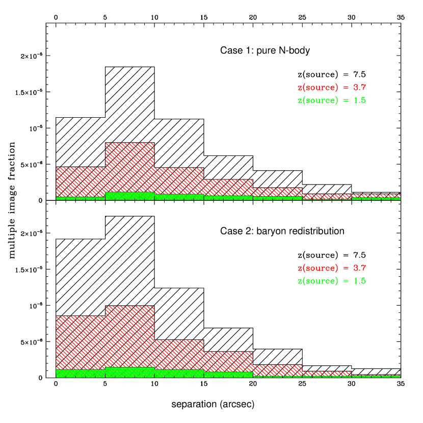
Figure 5: Frequency of multiple images as a function of separation (binned with 5 arcsec width). The number of multiple images clearly increases with decreasing splitting angle; the drop in the smallest separation bin is due to the fact that we are highly incomplete for splitting angles below 3 arcseconds. The N-body case is shown in the top panel, the scenario with baryon redistribution in the bottom panel. The histograms reflect three different source redshifts: z_s = 7.5 (highest, black, loose shading), z_s = 3.7 (middle, red, intermediate shading), z_s = 1.5 (lowest, green, densest shading). In the baryon redistribution scenario we find more multiple images (on average about 25%); this is most pronounced in the small separation regime.

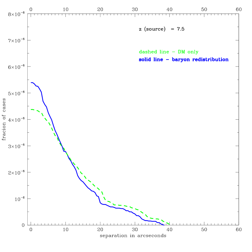
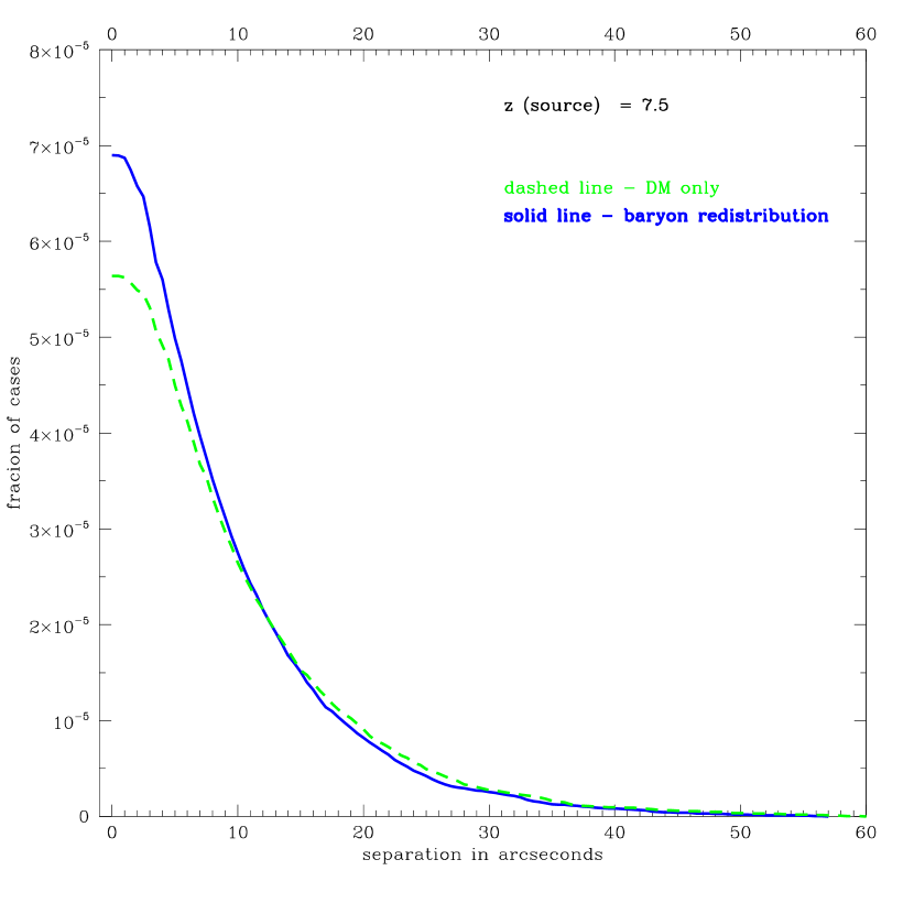
Figure 6: Integrated probability distribution of multiple images as a function of separation for a dark matter only simulation (green dashed line) and with baryon redistribution as described in the text (blue solid line). Top panel: For a source redshift of $z_{s}=1.5$; middle panel: $z_{s}=3.7$; bottom panel: $z_{s}=7.5$.

With the rearrangement, the number of multiple images increased for all source redshifts, particularly for angular separations up to 15 arcsec. This is shown in Figure 5; where the multiple image cases are binned according to the image splitting using bin widths of 5 arcsec (note we are highly incomplete in the first bin, because we do not properly resolve image splittings smaller than about 3 arcseconds). The level of increase can be read off of the integrated distributions in Figure 6, where the dashed lines show the integrated frequency of multiple images as a function of separation for the pure N-body case, and the solid lines show the scenario with baryon rearrangement. Qualitatively, it is obvious that including the baryon redistribution produces more multiple images. The amount by which the rearranged case is higher than the pure $N$-body case is almost independent of source redshift: the fraction is about 25% for the redshift range $z_{s}=1.5$ to $7.5$ (it varies between 22% and 28%). Beyond the total lensing frequencies, it is interesting to study the differential effect: it is for relatively small separations ($\leq 10$ arcmin) in particular that the baryon-redistribution case leads to more multiple images: about a 70% increase in the lowest bin, and 30% increase in the 5–10 arcsecond bin. This excess decreases with increasing separation, such that at a splitting of $\sim 12$ to $15$ arcsec the two cases result in the same frequencies for multiple images. This effect is easy to understand: the baryon redistribution steepens the innermost parts of the density profiles of halos, and hence can bring DM halos which are originally just below the critical density for lensing above this value, thus producing multiple images.

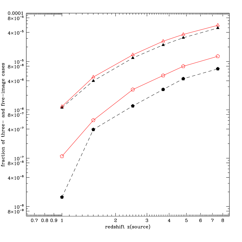
Figure 7: Image multiplicity as a function of source redshift for ”triple” images (triangles) and ”quintuple” images (pentagons). The pure N-body case is shown with solid symbols and dashed lines, for the baryon-rearrangement case we used open symbols and solid lines.

At still larger separations, the baryon redistribution case apparently produces slightly fewer cases (at the few percent level). The reason for this is not quite so obvious; in fact, it is rather counter-intuitive: if a fraction of the total mass becomes more concentrated, the total mass inside an image pair should be the same or larger. The explanation is that this effect is just an artifact of our definition of image separation. As described above, we define the separation of a multiple image system as the angular distance between the brightest and the third-brightest image. Our method always identifies the “odd” image in triples and quintuples, although in practice most would be identified as double and quadruple images, because the odd images in most observational situations are demagnified and not detectable (hence we refer subsequently to those cases as ”doubles” and ”quadruples”). A detailed look at the distribution of multiple images shows that a side effect of the redistribution of baryons is that the number of quadruple images increases more strongly than the number of doubles (see Figure 7). We are able to verify this by comparing individual lines of sight, with and without the matter rearrangement. When we compare one-to-one a situation that produces a double image in the DM-only scenario and a quadruple image in the baryon-redistribution case, the additional image pair occasionally is brighter than the faint “odd” image, and it happens that this pair is close to the brightest image of the multiplet, resulting in a smaller measured separation than in the pure N-body case. This leads to the apparent small deficit of large separation cases in the redistributed-baryon case.

3.2 Comparison with observations

Over the last decade, various papers have investigated the observational occurrence of giant arcs statistically, e.g. Luppino et al. (1999), Gladders et al. (2003), and Sand et al. (2005). The frequency of arcs reported in these studies varies from one giant arc per 45 deg² to about one arc per 10 deg²; the large spread may be explained partly by the slightly different definition and limiting magnitude, and may be related to the relatively small number of cases per study. Overall, just about 50 arc systems had been used for these statistical analyses, found in various surveys with diverse selection criteria.

Two recent studies based on SDSS data present quite different results as well. On one hand, Estrada et al. (2007) report no arcs found in a systematic investigation of 825 SDSS clusters (other than one serendipitous discovery). On the other hand, Hennawi et al. (2006) presented first results from a new survey for giant arcs, which may as much as double the number of known arcs (about 30 new systems already reported). This study is very promising not just due to the large number of new arc systems to be expected, but – at least as importantly – also by the fact that it will find them by well defined selection criteria.

Until these future results will be published, we can compare our results here (although only “differentially”) to those in Wambsganss et al. (2004). There it was found that the simulated pure N-body based arc frequencies are consistent with the observations, if we allow the source redshifts to extend well beyond $z\geq 1$ (as the distribution of observed arcs is as well). The result presented here— that by including the baryon rearrangement the predicted number of arcs increases by about 25%— puts the predicted arc frequency a bit on the high side, though still with considerable uncertainty both on the observational (e.g., absolute numbers, selection criteria) and the theoretical side (e.g., parameters of underlying cosmological model, exact definition of “arc”). Furthermore, the model used here has a high normalization for the amplitude of fluctuations as compared to the recent results from WMAP; a lower normalization would significantly reduce the lensing frequency (Li et al., 2007).

4 Summary and Conclusion

This paper quantitatively investigates the effects on lensing of baryon redistribution in originally pure dark matter $N$-body simulations. We describe a heuristic recipe for rearranging the baryons in dense dark matter halos that is consistent with observational data for massive galaxies, present a number of tests of this prescription, and then apply it to a cosmological simulation used for multiple lens plane ray shooting. We compare the frequency of multiple images, the image separation and the image multiplicity between the original $N$-body matter distribution and the redistributed version. We find that on average the case taking into account the redistribution of baryons produces 25% more multiple images; this is almost independent of the source redshift in the range $z_{s}=$ 1.5 to 7.5. For splittings between 5–10 arcseconds, the number of multiple images increases by roughly 30%, and by 70% for smaller separations $<5$ arcsecond. But this last result must be treated with caution since we are resolution limited for splittings $\lesssim 3$ arcsecond. As noted, most of the new multiple images systems occur for angular scales $\leq 10$ arcseconds. We also find that the number of quadruple images increases more than the number of double images. This produces an apparent slight reduction of larger separation cases, which is in fact only an artifact of the way we define image separation, namely as the distance between the brightest and the third-brightest image. Since arc statistics are such a good tool for distinguishing between models with different cosmological parameters, we would like to emphasize once again the need for both very good observational studies and for more explorations of the important parameters in the simulations.

Figure 1: The circular velocity profile of an example halo, demonstrating the effect of redistribution. Solid line: initial circular velocity. Dotted line: after mass removal (cf. Eqn. 6). Dot-dashed line: velocity of the isothermal component (cf. Eqn. 7). Dashed line: the final circular velocity profile.

Figure 2: Solid lines: stellar mass function as determined with the recipe described in the text, at redshifts $z$=0.05, 0.55, and 1.05 (top to bottom). The lower dotted line is taken from the SDSS luminosity function (Blanton et al. 2003, Gavazzi et al. 2007), assuming $M_{star}/L=4.4$; the upper dotted line instead assumes $M_{star}/L\propto L^{0.25}$.

Figure 3: The total rearranged “stellar” mass as a function of redshift (determined by applying the baryon redistribution recipe described in Section 2.1). The solid line is an empirically based estimate of the total mass in elliptical galaxies from Nagamine et al. (2006); the dashed line is limited to systems with $V_{c}>215$km/s, which would produce a splitting angle of $>$3”.

Figure 4: Top panel: Circular velocity $V$ at $R_{A}$ as a function of stellar mass $M_{\mathrm{s}tellar}$, for halos identified in the $z$=0.05 and 0.17 lens planes. The line is the circular velocity measured at 2.2 disk lengths by Pizagno et al. (2005). Bottom panel: Half-mass radius $R_{1/2}$ of the redistributed mass as a function of stellar mass $M_{\mathrm{s}tellar}$. The line is the Sersic half-light radius of early type galaxies from SDSS, see Shen et al. (2003).

References

- Bahcall & Bode (2003) Bahcall, N. A. & Bode, P. 2003, ApJ, 588, 1
- Bahcall & Cen (1993) Bahcall, N.A. & Cen, R. 1993, ApJ, 407, L49
- Bartelmann et al. (1998) Bartelmann, M., Huss, A., Colberg, J.M., Jenkins, A., & Pearce, F.R. 1998, A&A, 330, 1
- Blanton et al. (2003) Blanton, M.R., et al. 2003, ApJ, 592, 819
- Bode & Ostriker (2002) Bode, P. & Ostriker, J.P. 2003, ApJS, 145, 1
- Cox (2000) Cox, A.N. 2000, Allen’s astrophysical quantities, 4th ed., New York: AIP Press, 625
- Dalal, Holder & Hennawi (2004) Dalal, N., Holder, G. & Hennawi, J.F. 2004, ApJ, 609, 50
- Eke, Cole & Frenk (1996) Eke, V.R., Cole, S. & Frenk C.S. 1996, MNRAS, 282, 263
- Estrada et al. (2007) Estrada, J., Annis, J., Diehl, H. T., Hall, P. B., Las, T., Lin, H., Makler, M., Merritt, K. W., Scarpine, V., Allam, S., Tucker, D. 2007, ApJ, 660, 1176
- Evrard et al. (2007) Evrard, A.E. , Bialek, J., Busha, M., White, M., Habib, S., Heitmann, K., Warren, M., Rasia, E., Tormen, G., Moscardini, L., Power, C., Jenkins, A.R. , Gao, L., Frenk, C.S. , Springel, V., White, S.D.M., Diemand, J. 2007, ArXiv Astrophysics e-prints, arXiv:astro-ph/0702241
- Gavazzi et al. (2007) Gavazzi, R., Treu, T., Rhodes, J. D., Koopmans, L. V., Bolton, A. S., Burles, S., Massey, R., & Moustakas, L. A. 2007, ArXiv Astrophysics e-prints, arXiv:astro-ph/0701589
- Gladders et al. (2003) Gladders, M., Hoekstra, H., Yee, H.K.C., Hall, P.B., & Barrientos, L.F. 2003, ApJ, 593, 48
- Hennawi et al. (2006) Hennawi, J. F., Gladders, M. D., Oguri, M., Dalal, N., Koester, B., Natarajan, P., Strauss, M. A., Inada, N., Kayo, I., Lin, H., Lampeitl, H., Annis, J., Bahcall, N. A., Schneider, D. P., ArXiv Astrophysics e-prints, arXiv:astro-ph/0610061
- Hennawi et al. (2007a) Hennawi, J. F., Dalal, N., & Bode, P. 2007a, ApJ, 654, 93
- Hennawi et al. (2007b) Hennawi, J. F., Dalal, N., Bode, P. & Ostriker, J.P. 2007b, ApJ, 654, 714
- Henry & Arnaud (1991) Henry, J.P. & Arnaud, K.A. 1991, ApJ, 372, 410
- Hilbert et al. (2007) Hilbert, S., White, S. D. M., Hartlap, J., & Schneider, P. 2007, ArXiv Astrophysics e-prints, arXiv:astro-ph/0703803
- Ho & White (2005) Ho, S., & White, M. 2005, Astroparticle Physics, 24, 257
- Horesh et al. (2005) Horesh, A., Ofek, E. O., Maoz, D., Bartelmann, M., Meneghetti, M., & Rix, H.-W. 2005, ApJ, 633, 768
- Inada et al. (2003) Inada, N., et al. 2003, Nature, 426, 810
- Inada et al. (2005) Inada, N., et al. 2005, PASJ, 57, L7
- Inada et al. (2006) Inada, N., et al. 2006, ApJ, 653, L97
- Jing et al. (2006) Jing, Y. P., Zhang, P., Lin, W. P., Gao, L., & Springel, V. 2006, ApJ, 640, L119
- Kauffmann et al. (2003) Kauffmann, G., et al. 2003, MNRAS, 341, 33
- Li et al. (2005) Li, G.-L., Mao, S., Jing, Y. P., Bartelmann, M., Kang, X., & Meneghetti, M. 2005, ApJ, 635, 795
- Li et al. (2006) Li, G. L., Mao, S., Jing, Y. P., Mo, H. J., Gao, L., & Lin, W. P. 2006, MNRAS, 372, L73
- Li et al. (2007) Li, G. L., Mao, S., Jing, Y. P., Lin, W. P. & Oguri, M. 2007, MNRAS, 378, L469
- Li & Ostriker (2002) Li, L.-X., Ostriker, J.P. 2002, ApJ, 566, 652
- Li & Ostriker (2003) Li, L.-X., Ostriker, J.P. 2003, ApJ, 595, 603
- Lin et al. (2006) Lin, W. P., Jing, Y. P., Mao, S., Gao, L., & McCarthy, I. G. 2006, ApJ, 651, 636
- Luppino et al. (1999) Luppino, G. A., Gioia, I. M., Hammer, F., Le Fevre, O., & Annis, J. A. 1999, ApJS, 136, 117
- Meneghetti et al. (2003) Meneghetti, M., Bartelmann, M., Moscardini, L. 2005, MNRAS, 346, 67
- Nagamine et al. (2006) Nagamine, K., Ostriker, J. P., Fukugita, M. & Cen, R. 2006, ApJ, 653, 881
- Oguri et al. (2004) Oguri, M., et al. 2004, ApJ, 605, 78
- Oguri & Keeton (2004) Oguri, M., & Keeton, C. R. 2004, ApJ, 610, 663
- Oukbir & Blanchard (1992) Oukbir, J., & Blanchard, A. 1992, A&A, 262, L21
- Peng et al. (2004) Peng, E.W., Ford, H., & Freeman, K. 2004 ApJ, 602, 685
- Pizagno et al. (2005) Pizagno, J., et al. 2005, ApJ, 633, 844
- Puchwein et al. (2005) Puchwein, E., Bartelmann, M., Dolag, K., Meneghetti, M. 2005, A&A, 442, 405
- Rozo et al. (2006) Rozo, E., Nagai, D., Keeton, C., Kravtsov, A. 2006, ArXiv Astrophysics e-prints, arXiv:astro-ph/069621
- Sand et al. (2005) Sand, D. J., Treu, T., Ellis, R. S., Smith, G. P. 2005, ApJ, 627, 32
- Sharon et al. (2005) Sharon, K., et al. 2005, ApJ, 629, L73
- Shen et al. (2003) Shen, S., Mo, H.J., White, S.D.M., Blanton, M.R., Kauffmann, G., Voges, W., Brinkmann, J. and Csabai, I. 2003, MNRAS, 343, 978
- Spergel et al. (2006) Spergel, D. N., Bean, R., Doré, O., Nolta, M. R., Bennett, C. L., Dunkley, J., Hinshaw, G., Jarosik, N., Komatsu, E., Page, L., et al. 2007, ApJS, 170, 377
- Turner (1990) Turner, E.L. 1990, ApJ365, 43
- Vale & Ostriker (2006) Vale, A. & Ostriker, J. P. 2006, MNRAS, 371, 173
- Viana & Liddle (1996) Viana, P.P. & Liddle, A.R. 1996, MNRAS, 281, 323
- Wambsganss et al. (1995) Wambsganss, J., Cen, R., Ostriker, J. P., & Turner, E. L. 1995, Science, 268, 274
- Wambsganss et al. (1997) Wambsganss, J., Cen, R., Xu, G., & Ostriker, J. P. 1997, ApJ, 475, L81
- Wambsganss et al. (1998) Wambsganss, J., Cen, R., & Ostriker, J. P. 1998, ApJ, 494, 29
- Wambsganss et al. (2004) Wambsganss, J., Bode, P., & Ostriker, J. P. 2004, ApJ, 606, L93
- Wambsganss et al. (2005) Wambsganss, J., Bode, P., & Ostriker, J. P. 2005, ApJ, 635, L1
- White, Efstathiou, & Frenk (1993) White, S.D.M., Efstathiou, G. & Frenk, C.S. 1993, MNRAS, 262, 1023