Instability of reconstruction of the low CMB multipoles

Abstract

We discuss the problem of the bias of the Internal Linear Combination (ILC) CMB map and show that it is closely related to the coefficient of cross-correlation $K(\ell)$ of the true CMB and the foreground for each multipole $\ell$. We present analysis of the cross-correlation for the WMAP ILC quadrupole and octupole from the first (ILC(I)) and the third (ILC(III)) year data releases and show that these correlations are $\sim-0.52-0.6$. Analysing $10^{4}$ Monte Carlo simulations of the random Gaussian CMB signals, we show that the distribution function for the corresponding coefficient of the cross-correlation has a polynomial shape $P(K,\ell)\propto(1-K^{2})^{\ell-1}$. We show that the most probable value of the cross-correlation coefficient of the ILC and foreground quadrupole has two extrema at $K\simeq\pm 0.58$. Thus, the ILC(III) quadrupole represents the most probable value of the coefficient $K$. We analyze the problem of debiasing of the ILC CMB and pointed out that reconstruction of the bias seems to be very problematic due to statistical uncertainties. In addition, instability of the debiasing illuminates itself for the quadrupole and octupole components through the flip-effect, when the even $\ell+m$ modes can be reconstructed with significant error. This error manifests itself as opposite, in respect to the true sign of even low multipole modes, and leads to significant changes of the coefficient of cross-correlation with the foreground. We show that the CMB realizations, whose the sign of quadrupole $(2,0)$ component is negative (and the same, as for all the foregrounds), the corresponding probability to get the positive sign after implementation of the ILC method is about $40\%$.

Key words:    cosmology: cosmic microwave background — cosmology: observations — methods: data analysis

1 INTRODUCTION

Since     the    COBE    experiment    and    then    after   the  Wilkinson     Microwave    Anisotropy Probe
(WMAP) [1, 2, 3, 4, 5, 6, 7] first and third year data releases, the problem of reconstruction of the CMB low multipoles $\ell\leq 10$ (including the power of a quadrupole, planarity and alignment of the quadrupole and the octupole etc.) attracts very serious attention. A lot of cosmological models have been involved for the explanation of the peculiarities of the ILC (Internal Linear Combination ) low multipoles including the model of running spectral index of the primordial adiabatic perturbations [1, 2, 3, 4, 5], non-trivial topology of the Universe [8, 9], Broken Scale Invariance (BSI) of the power spectrum [10, 11], primordial magnetic field [12, 13, 14], Bianchi VIIh cosmological model [15, 16, 17, 18, 19], etc.

The problem of low power of the CMB quadrupole can be related to the non-Gaussianity of the WMAP low multipoles, including planarity and alignment of the quadrupole and octupole [20, 21, 22, 23], cross–correlations with the foregrounds [24, 25, 26, 4, 27], local defects of the CMB map [28], etc. These peculiarities need some theoretical explanation, since the origin of those non-Gaussian features still remains unknown.

Another way to look at the problem of the low multipole range of the ILC CMB signal is to take under consideration the cross-correlation between the CMB signal and the foregrounds, known as a bias of the ILC map [29, 4, 27, 24, 30], some effects of systematics [31] including contamination of the $\ell=2$ mode by dipole through far sidelobes [32].

In this paper we would like to re-examine one of the most important issues of the data analysis of the modern CMB experiments related to the problem of the CMB–foreground separation by the ILC Method. Needless to say, that separation of the CMB signal and foregrounds is the major problem for all the CMB experiments including the ongoing WMAP and the future Planck missions. The basic formalizm of the ILC method which allows one to reconstruct the CMB signal from the observational data sets is to combine the data in one (Linear Combination) map by using real weighting coefficients. Then, to find these weighting coefficients, we need to minimize some functional defined on multifrequency CMB data sets containing information about the primordial CMB signal, the instrumental noise and the foregrounds. This functional (particularly, variance by Tegmark and Efstathiou [33] (hereafter TE)) can be defined both in the pixels domain (like it was done by the WMAP team), and in the spherical harmonics domain [34] (hereafter TOH), and [4, 30, 35]. Below, we will discuss only the low CMB multipoles ($\ell\leq 10$) and, particularly, the quadrupole for which the ILC approach in multipole domain seems to be very useful.

However, the ILC approach in combination with the Minimal Variance Method (hereafter, ILC MVM) produces a specific feature of the derived CMB signal, known as the bias. The bias reflects directly the cross-correlation with foregrounds, and leads to the non-Gaussianity and statistical anisotropy of the derived CMB through coupling with the foreground. This is because the MVM was originally designed for separation of the Gaussian signals, of which the statistical properties are completely specified by the variance of each component. At the same time, it is well known in the data analysis that the MVM is not motivated properly, especially in cases when we have only a unique realization of the random process, where the CMB signal is mixed with the significantly non-Gaussian foreground. Moreover, the statistics of the low multipoles of the CMB signal are extremely peculiar, since we do not have the statistical ensemble of realizations.

In general, this paper is devoted to investigation of the ILC bias and its statistical uncertainties. We will show that so-called debiasing of the ILC CMB has potential instabilities and unpredictability for a single realization of the CMB.

The outline of the paper is as follows. In Section 2, we focus our attention on mathematical basis of the ILC MVM exactly in the same way as it was proposed by [4]. By analysis of the model with homogeneous foreground spectra, we show that the bias of the ILC image, and the bias of the power spectrum are in order of $K(\ell)$ and $K^{2}(\ell)$, where $K(\ell)$ is the coefficient of “the true CMB — true foreground” cross-correlation. Following [26], we will call this cross-correlation “the cosmic covariance”. Because of statistical origin of this correlation, the cosmic covariance is uncertain for each single realization of the CMB signal, even for well known foregrounds. At the same time, derived by the ILC MVM, the ILC CMB signal and corresponding ILC MVM foregrounds have zero cross–correlations due to design of the ILC  MVM.

In Section 3, we draw our attention to the investigation of the statistical properties of the coefficient of cross-correlation between the random Gaussian CMB and the WMAP foregrounds for K–W bands. We generate $10^{4}$ realizations of the Gaussian CMB signals for the WMAP best fit $\Lambda$CDM cosmological model, and cross-correlate them with the foregrounds obtained by the WMAP team (the Maximum Entropy Method (MEM) foregrounds, which constitute as a sum of the synchrotron, free-free and dust emission for each frequency band). We will show, that the probability distribution function for these cross-correlations has a polynomial shape $P(K,\ell)\propto(1-K^{2})^{\ell-1}$. After that, we will find the most probable values of the coefficients $\overline{K}(\ell)$ and $\overline{K}^{2}(\ell)$. In another words, these coefficients determine the most probable value of the bias for the ILC CMB and the power spectrum. Taking under consideration that the maps ILC(III) of three years and ILC(V) of five years data are already debiased, as the WMAP team claimed, we check out the cross-correlation between the ILC and the WMAP forground. After debiasing, these cross-correlations should represent the possible value of the $K(\ell)$ for the true CMB and the true foreground. For the WMAP K-W bands, the corresponding coefficients of the cross–correlations are about $K\simeq-0.51$. Remarkably, this value is close to the most probable value $\overline{K}(\ell)$ of the distribution function $KP(K,\ell=2)$.

In Section 4 we discuss some peculiarities of the ILC(III) quadrupole and the octupole. As it follows from the Monte Carlo simulations presented in [36] for low multipoles $\ell=2,3$, the sign of the ($\ell=$2,$m=$0), (2,2) and (3,1) components was changed to the opposite one for about 20% of the output CMB maps. This flip-effect significantly changed the morphology of the output CMB map. We will show that the flip-effect takes place for those input CMB quadrupoles, for which the sign of $\ell=2,m=0$ mode is opposite to the sign of the foreground. For the Gaussian CMB signal about 50% of the realizations have ${\rm sign}~{}c_{2,0}=-{\rm sign}~{}F_{2,0}$, where $c_{2,0}$ and $F_{2,0}$ are the $m$=0 components of the quadrupole for the input CMB and the foreground, respectively. Roughly for $40\%$ of those realizations, reconstruction of the $\ell=2,m=0$ component could have a wrong sign of the (2,0) mode. In this Section we present some analytical description of the flip-effect based on the properties of the bias.

We summarize our results in Conclusion.

2 MATHEMATICAL BASIS OF THE ILC MVM METHOD

Let us draw our attention to the general formalism of the ILC method, assuming that we have experimental data $\Delta T(\theta_{p},\phi_{p},\nu_{i})$ for the CMB anisotropy obtained for some frequency bands $\nu_{1},\nu_{2}...$. Here $\theta_{p}$ and $\phi_{p}$ are the standard polar and azimuthal angles of the spherical coordinate system and the index $p$ mark a corresponding pixel. The observed sky temperature for each pixel $p$ in a given band $i$ is the linear combination of the true CMB signal $T_{c}(p)$ and the true foreground $f_{i}(p)$. In reality, the components of the foreground at different frequency bands (mainly the synchrotron, the free-free and the dust emission) have angular variations of the spectral indicies. However, by using different disjoint regions of the sky with nearly uniform foreground spectra and low level of spatial variations we can simplify the mathematical basis of the ILC method [4]. Following the WMAP model of the foregrounds, let us assume that for some region of the sky the spatial variation of the foregrounds emission are negligible and $f_{i}(p)=S_{i}F(p)$, where $S_{i}$ is the frequency spectrum and $F(p)$ is the spatial distribution of the foreground for each band $i$. The main idea of the ILC method is to estimate the CMB signal by using real weighting coefficients $w_{i}$ for each region of the sky with monotonic spectrum of the foreground [4]

$$\small{T_{ilc}(p)=\sum_{i}w_{i}T_{i}(p)=T_{c}(p)+\Gamma F(p),\sum_{i}w_{i}=1,}$$ (1)

where $\Gamma=\sum_{i}w_{i}S_{i}$. The coefficients $w_{i}$ can be found by minimization of the variance (see [4])

$$\sigma^{2}_{ilc}=\langle T^{2}_{ilc}(p)\rangle-\langle T_{ilc}(p)\rangle^{2}$$

$$=\sigma^{2}_{c}+2\Gamma\sigma_{cF}+\Gamma^{2}\sigma^{2}_{F}.\hskip 17.07182pt$$ (2)

Here $\sigma^{2}_{c}$ is the variance of the true CMB, $\sigma^{2}_{F}$ is the variance of the true foreground and

$$\sigma_{cF}=\langle T_{c}(p)F(p)\rangle-\langle T_{c}(p)\rangle\langle F(p)\rangle$$

is the cosmic covariance between the true CMB and the foreground [26]. The angle brackets in Eq.2 and hereafter denote the averages over the pixels belonging to each zone of the map with the monotonic spectrum of the foreground. The minimum of the variance $\sigma^{2}_{ilc}$ can be easily found from the equation $\frac{d\sigma^{2}_{ilc}}{dw_{i}}=0$, whence we get [4]

$$T_{ilc}(p)=T_{c}(p)-\frac{\sigma_{cF}}{\sigma^{2}_{F}}F(p),\hskip 2.84544pt\sigma^{2}_{ilc}=\sigma^{2}_{c}-\frac{\sigma^{2}_{cF}}{\sigma^{2}_{F}}.$$ (3)

Let us define the coefficient of cross-correlation between the true CMB signal and the true foreground as

$$\kappa=\frac{\sigma_{cF}}{\sigma_{c}\sigma_{F}}.$$ (4)

Then,   after   substitution   of   Eq.(4)   in   Eq.(3)   we have [26]:

$$T_{ilc}(p)=T_{c}(p)-\kappa\frac{\sigma_{c}}{\sigma_{F}}F(p),\hskip 2.84544pt\sigma^{2}_{ilc}=\sigma^{2}_{c}(1-\kappa^{2}).$$ (5)

As one can see from Eq.(5), the temperature per pixel $T_{ilc}(p)$ and the variance $\sigma^{2}_{ilc}$ are biased. For $T_{ilc}(p)$ the difference $T_{ilc}(p)-T_{c}(p)$ is proportional to the $\kappa$ and can be both positive and negative. For the variance $\sigma^{2}_{ilc}$, the bias is always negative and proportional to $1-\kappa^{2}$. The existence of such a bias is not supprising. The shift of the ILC variance and corresponding power spectrum was discussed in [4, 29, 27, 26]. However, it would be important to note that the bias of the variance and the power spectrum is determined by the cosmic covariance, which is unknown for each single realization of the CMB sky. This is the reason why it can not be corrected by any methods because of the statistical uncertainties.

Table 1: The table of $K_{ff}(\ell)$ coefficients for “V–W”, “Ka–V”, “Ka–W” and “Q–V” MEM foregrounds. The first column indicates the multipole $\ell$.

$K_{ff}(\ell)$	$V-W$	$Ka-V$	$Ka-W$	$Q-V$
2	0.999969	0.999014	0.998761	0.999481
3	0.994699	0.999534	0.995187	0.999770
4	0.996702	0.999497	0.996098	0.999708
5	0.994615	0.998862	0.995825	0.999647
6	0.995481	0.999354	0.993799	0.999563
7	0.993245	0.998620	0.995323	0.999506
8	0.994281	0.999252	0.993458	0.999575
9	0.993532	0.998781	0.994617	0.999571
10	0.994638	0.999068	0.993319	0.999463

The ILC approach presented above in the pixel domain can be easily generalized for the multipole domain by spherical harmonics decomposition: $\Delta T(\theta,\phi,\nu_{i})\rightarrow a^{\nu_{i}}_{\ell,m}$:

$$\Delta T(\theta,\varphi,\nu_{j})=\sum_{\ell=0}^{\infty}\sum_{m=-\ell}^{\ell}|a^{\nu_{j}}_{\ell,m}|e^{i\phi_{\ell,m}}Y_{\ell m}(\theta,\varphi),$$ (6)

where $|a_{\ell m}|$ and $\phi_{\ell,m}$ are the moduli and phases of the coefficients of the expansion. Direct conversion of Eq.(5) to the multipoles coefficients gives us

$$\overline{c}^{ilc}_{\ell,m}=c_{\ell,m}-\kappa\frac{\sigma_{c}}{\sigma_{F}}F_{\ell,m}.$$ (7)

It is easy to show that this solution for the derived ILC signal $\overline{c}^{ilc}_{\ell,m}$ can be obtained by minimization of the variance

$$\sigma^{2}=\sum_{\ell}\frac{2\ell+1}{4\pi}\sum_{m=-\ell}^{\ell}|\sum_{j}w_{j}a^{j}_{\ell,m}|^{2}.$$ (8)

Moreover, follow to TOH approach we can define the ILC CMB in multipole domain by using weighting coefficients $W_{i}(\ell),\sum_{i}W_{i}(\ell)=1$ and minimizing the power spectrum for each multipole

$$C(\ell)=\sum_{m}|W_{i}(\ell)a^{(i)}_{\ell,m}|^{2}.$$

For the model of uniform spectra of the foreground this approach leads to

$$c^{ilc}_{\ell,m}=c_{\ell,m}-K(\ell)\frac{(\sum_{m=-\ell}^{\ell}|\overline{c}_{\ell,m}|^{2})^{\frac{1}{2}}}{\left(\sum_{m=-\ell}^{l}|F^{(2)}_{\ell,m}|^{2}\right)^{\frac{1}{2}}}F^{(2)}_{\ell,m},$$ (9)

where $K(\ell)$ is the coefficient of cross-correlation between the ILC CMB and the foreground:

$$K(\ell)=\frac{\sum_{m}\left(c^{ilc}_{\ell,m}F^{*}_{\ell,m}+(c^{ilc})^{*}_{\ell,m}F_{\ell,m}\right)}{2\left[\sum_{m}|c^{ilc}_{\ell,m}|^{2}\sum_{m}|F_{\ell,m}|^{2}\right]^{\frac{1}{2}}}.$$ (10)

Taking Eq.(9) and Eq.(10) into account, one can get

$$C^{ilc}(\ell)=C_{c}(\ell)\left[1-K^{2}(\ell)\right].$$ (11)

Before any future analysis, let us draw our attention to the applicability of the model of the uniform foreground spectra, taking the MEM foregrounds in K–W bands of the WMAP data into account. For these foregrounds (sum of the synchrotron, free-free and dust emission for each frequency band) the coefficient of cross-correlation is defined in the same way as Eq.(10) with substitution of $F^{(j)}_{\ell,m},F^{(k)}_{\ell,m}$ for $c^{ilc}_{\ell,m},F_{\ell,m}$ in Eq.(10).

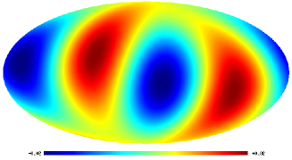
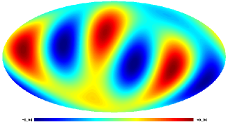
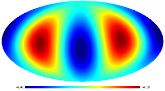
Figure 1: The quadrupole component of the ILC(I) (top left), the ILC(III) quadrupole (middle left) and the difference between them (bottom left). Right column is for the ILC(I), ILC(III) and difference of octupole.

In Table 1 we show the coefficients of cross-correlation for different combination of the WMAP MEM foregrounds. One can see that corresponding coefficients of cross-correlation between different foregrounds (for different bands) are extremely close to unity. Thus the model of uniform spectra of the foreground is very well motivated. As it follows from Eq.(9) and Eq.(11), the corresponding bias of the ILC coefficient $c^{ilc}_{\ell,m}$ is proportional to the $K(\ell)$, while the bias of the power spectrum is of the order of $K^{2}(\ell)$. Since the true CMB constitute as a random (Gaussian ?) process, the coefficient of cross-correlation $K(\ell)$ represents a random (non-Gaussian) process as well. Thus, for each particular realization of the CMB sky, the coefficient of cross-correlation $K(\ell)$ remains uncertain. Note that the WMAP team, as mentioned in [27], to correct the CMB power obtained by the ILC method took under consideration $10^{2}\div 10^{4}$ realizations of the random Gaussian CMB, creating the statistical ensemble of realizations. However, even after the averaging over realizations we can not predict the bias for one particular realization of the CMB due to the cosmic covariance. Moreover, as it is seen from Eqs.(9) and (11), the average of the ILC CMB signal over the ensamble of realization reduces the bias factor $\langle K\rangle$ down to zero, while $\langle K^{2}\rangle\neq 0$. Thus, for the ensemble of realization the correction of the CMB power can be done successfully, while the correction of the signal itself seems to be very problematic.

One more problem is related to the statistical properties of the true CMB signal. As it is well known, the low multipoles ($\ell\leq 10$) of the WMAP CMB signal reveal significant departure from the statistical isotropy and homogenity [36, 37]. If this effect is the manifestation of the primordial non-Gaussianity of the CMB, we simply do not have the correct model of the statistical ensemble of realizations. This remark illuminates significantly stronger the problem of instability of the reconstruction of the low multipoles of the CMB signal.

Not to be able to give the general solution of the problems mentioned above, we would like to propose indirect method of evaluation of the bias in the image and power domains by looking at the cross-correlation coefficient $K(\ell)$ of the derived CMB signal and the MEM foregrounds, including the the synchrotron map of Haslam et al. [38] (hereafter HA). The idea is based on the fact that in Eq.(5) the cross-correlation of the ILC and the foreground is exactly zero. Thus, if by implementation some methods of debiasing of the ILC map we will get $K\neq 0$, it would be reasonable accurate estimator of the initial coefficient of cosmic covariance $\kappa$. In next section we will discuss this approach in details.

3 THE ILC(I) AND ILC(III) CROSS-CORRELATIONS WITH THE FOREGROUNDS

As was pointed out by the WMAP team [4] the correction of the ILC CMB can be done by implementation of additional information about the foregrounds and 100 realizations of the random Gaussian CMB signals, which mimic the WMAP K-W bands in combination with MEM foreground. Repeating the ILC MVM method for each from these 100 realization, the WMAP team took under consideration some systematic of the ILC method and made corresponding correction of the derived the ILC(III) map.

Figure 2: Top. The coefficient of cross–correlation of the ILC(I) and ILC(III) with the foregrounds. The dash line is for the ILC (III) and the Haslam et al. map (1982); the triple dots dash line is for the ILC(I) and Haslam et al. map; the thick solid line with stars is for the cross-correlation of ILC(I) and V-band MEM foreground. The dash line with diamonds is for the ILC(III) and the V-band MEM foreground. Bottom. The coefficients of cross-correlations between V- and W-foregrounds of the WMAP (the thick solid line), V- and Haslam et al. 1982 (the dash line) and finally ILC(I) and ILC(III) (the triple dots–dash line). The dash line is for Q- and V-bands, the stars are for Ka–V and the boxes are for Q–V foregrounds.

It is important to note that the WMAP team [4] pointed out that difference between the ILC(III) and the ILC(I) is mainly due to the bias. In Fig. 1 we show the quadrupole and the octupole components of the ILC(I) and the ILC(III) maps and difference between them to illustrate the correction of the bias made by the WMAP team for low multipoles range of the signal.

Let us draw our attention to the cross-correlation of the ILC(I) and ILC(III) maps with the MEM foregrounds (being the sum over synchrotron, free–free and dust emission maps). In Fig. 2 we show the coefficient of the ILC-foreground cross-correlation $K(\ell)$ for the multipoles $\ell=2-10$ and for the WMAP MEM foreground for K–W band. In addition in Fig. 2, we show $K_{j}(\ell)$ for the ILC(I), the ILC(III), and the Haslam et al. synchrotron map [38]. As one can see from this figure, the quadrupole $(\ell=2)$ and $\ell=5$ multipole of the ILC(III) have negative correlation ($K\sim-0.5$) with Ka–W foregrounds. Moreover, the ILC(III) quadrupole has $K\sim-0.6$ with the Haslam et al. quadrupole.

3.1 Statistical properties of the bias

To understand the properties of the ILC(III)—foreground cross-correlation, we performed numerical test taking under consideration 10000 realizations of the random Gaussian CMB maps and cross-correlate them with the same model of the foregrounds as in Fig. 2 without any debiasing.

In Fig. 3 we show the probability density function $P(K_{j}(\ell))$ versus $K_{j}(\ell)$ for the multipoles $\ell=2\div 10$.

Figure 3: The distribution function $P(K)$ for cross–correlation between random CMB and the V-band foreground (left). From the top left down to the bottom right $\ell=2,3..10$. Note that the shape of $P(K)$ is the same for any foreground from K–W band including Haslam et al. (1982) signal.

For the input random Gaussian CMB signal the shape of the distribution functions is perfectly fitted by the function

$$P(K,\ell)=A_{\ell}(1-K^{2})^{\ell-1},$$ (12)

where $A_{\ell}$ is the normalization constant. Using $P(K,\ell)$ for the input signal shown in Fig. 3 (top left), we have found the first $<K>=-0.00043$ and the second $<K^{2}>=0.19934$ moments of $P(K,\ell=2)$, which is in agreement with corresponding value $<K^{2}>=0.2$ from Eq.(12).

Figure 4: The distribution functions $KP(K)$ (top) and $K^{2}P(K)$ (middle) for cross–correlation between random realizations of the CMB signal and the V band foreground. Bottom plot shows the distribution of $\langle K^{n}(\ell)\rangle$ for $\ell=2-10$. The solid line corresponds to $\langle K^{2}(\ell)\rangle$, the dash line is for $\langle K^{4}(\ell)\rangle^{\frac{1}{2}}$, the stars are for $\langle K(\ell)\rangle$, the rhombuses are for $\langle K^{3}(\ell)\rangle$.

Table 2: The table of $S$ coefficients for 10000 realizations of the CMB input and output maps. The top row contains data for the quadrupole component, the bottom one does for the octupole. $\Re$ and $\Im$ mark real and imaginary parts of the $a_{\ell,m}$ coefficients.

$\ell=2$	$2,0$	$\Re(2,1)$	$\Im(2,1)$	$\Re(2,2)$	$\Im(2,2)$	-	-
$S=-1$	2148	361	55	1756	257	-	-
$\ell=3$	$(3,0)$	$\Re(3,1)$	$\Im(3,1)$	$\Re(3,2)$	$\Im(3,2)$	$\Re(3,3)$	$\Im(3,3)$
$S=-1$	232	1852	337	106	367	533	355

At the end of this section we would like to present the distribution functions for the first and second moments of the coefficient of cross-correlation between the Gaussian realizations of the CMB signal and the foreground. These moments determine the bias of the ILC signal and the power spectrum. It is not supprising that the first, $KP(K)$ and the second $K^{2}P(K)$ moments shown in Fig. 4, have two points of extrema, which can be easily estimated from Eq.(12):

$$K^{n,\ell}_{\pm}=\pm\left(\frac{n}{2(\ell-1)+n}\right)^{\frac{1}{2}},$$ (13)

where $n$ is the order of moment $K^{n}P(K)$, and $\ell$ is the multipole number. For $\ell=2$ and $n=1$ we have $K^{1,2}=\pm 0.577$ and $K^{2,2}=\pm 0.707$. This result clearly demonstrates that if the sign of $\kappa$ coefficient is fixed, the most probable values of $K$ is $K^{1,2}$, and the most probable vale of $K^{2}$ is $K^{2,2}$. The bottom plot of Fig. 4 shows the value of the moments $M(n)=\langle K^{n}P(K,\ell)\rangle$ for the ensemble of realization of the random Gaussian process. For the second moment $n=2$ the shape of the function $M(n)$ is $(2\ell+1)^{-1}$, in agreement with estimation [27] of the bias of the power spectrum. From Eq.(13) one can find the most probable value of $K^{2}$ for the quadrupole component $K^{2}_{prob}=0.5$. This means that the most probable value of the factor $(1-K^{2}_{prob})$ is 0.5, and then from Eq.(11), we get $C_{c}(\ell=2)=2C_{ilc}(\ell=2)$. At the same time the most probable value of the bias of the ILC CMB is determined by the parameter $\kappa=K^{1,2}=\pm 0.577$. One can see that this value is remarkably close to the WMAP ILC(III) coefficient of the cross-corelation with the foreground.

4 PECULIARITIES OF QUADRUPOLE END OCTUPOLE

In addition to the cross-correlation with the foreground, we have discovered one more feature of the ILC method, which could have a significant impact on solution of the problem of the ILC(III) quadrupole [39]. We call this effect as a flip of the sign of the (2,0) component of the ILC quadrupole with respect to the sign of the true CMB (2,0) component. To understand quantitatively this effect, let us come back to Eqs.(9) and (10) for the quadrupole component $\ell=2$ and take under consideration the $(2,m=0)$ mode:

$$|c^{ilc}_{2,0}|\cos(\xi_{2,0})=|c_{2,0}|\cos(\eta_{2,0})$$

$$-\kappa\left[\frac{\sigma_{c}}{\sigma_{F}}\right]^{\frac{1}{2}}|F_{2,0}|\cos(\phi_{2,0}),\hskip 17.07182pt$$ (14)

where $|..|$ denotes the modulus, and $\xi_{2,0},\eta_{2,0}$ and $\phi_{2,0}$ are the phases of $2,0$ component of the ILC quadrupole, the true quadrupole, and the foreground correspondingly. Since the $m=0$ mode has the only real part, these phases simply mean the sign of the (2,0) components. For our further analysis it is important to note that for all K–W foregrounds $|F_{2,0}|\gg|F_{2,1}|,|F_{2,2}|$ and $\phi_{2,0}=\pi$. Taking into account Eq.(10), one can easily find that

$$\kappa\simeq-\frac{|c_{2,0}||F_{2,0}|\cos(\eta_{2,0})}{\sigma_{c}\sigma_{F}}(1-\varepsilon),$$

$$\varepsilon=\frac{2\sum_{m=1}^{2}|c_{2,m}||F_{2,m}|\cos(\eta_{2,m}-\phi_{2,m})}{\cos(\eta_{2,0})|c_{2,0}||F_{2,0}|},$$ (15)

where $\eta_{2,m},\phi_{2,m}$ are the phases of the true CMB and the foreground with $m=1$ and $m=2$ components of the quadrupole. Thus, after substitution of $\kappa$ from Eq.(15) into Eq.(14), we get

$$|c^{ilc}_{2,0}|\cos(\xi_{2,0})=|c_{2,0}|\cos(\eta_{2,0})\frac{\mu+\varepsilon}{1+\mu},$$ (16)

where

$$\mu=(|F_{2,1}|^{2}+|F_{2,2}|^{2})/|F_{2,0}|^{2}\ll 1.$$

From Eq.  (16) one    can   get   that   if    $\varepsilon\ll\mu$,    then $\xi_{2,0}=\eta_{2,0}$   and   $|c^{ilc}_{2,0}|=\mu|c_{2,0}|\ll|c_{2,0}|$. Thus, the ILC $|c^{ilc}_{2,0}|$ mode is smaller than corresponding $|c_{2,0}|$ by the factor $\sim\mu$. However, if $\varepsilon\gg\mu$, we have

$$|c^{ilc}_{2,0}|\cos(\xi_{2,0})\hskip 122.34692pt$$

$$\simeq 2\frac{\sum_{m=1}^{2}|c_{2,m}||F_{2,m}|\cos(\eta_{2,m}-\phi_{2,m})}{|F_{2,0}|}$$ (17)

and now the phase $\cos(\xi_{2,0})$ is determined by the sign of the nominator of the right part in Eq.(17). This result tells us that for some of realizations of the random CMB, the sign of the input signal is no matter. The reconstructed ILC phase $\xi_{2,0}$ can be the same $(\eta_{2,0})$, or opposite $\eta_{2,0}\pm\pi$ to the phase of the true CMB.

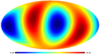
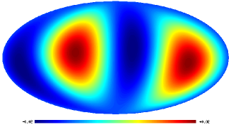
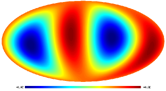
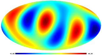
Figure 5: The illustration of the flip-effect for the ILC(III) quadrupole and octupole. Top is the ILC(III) quadrupole, the second from top is the ILC(III) quadrupole with flip-effect of the (2,0) component, the third from the top is the quadrupole with flip-effect of the (2,2) component. The second from the bottom and the bottom panels show the ILC(III) octupole and the flip-effect for the (3,1) octupole component.

To show that this effect takes place in numerical simulations of the ILC method, we consider the 10000 realization input and output maps for the $c_{2,0}$ quadrupole component, presented in [36]. As was pointed out in [4], the difference between the WMAP and Eriksen et al. approach [36] for derived CMB signals is caused by different choice of disjoint regions in the Galactic plane area, rather than the different bias. Using an estimator

$$S=s^{in}_{2,0}\cdot s^{out}_{2,0}=\cos\eta^{in}_{2,0}\cdot\cos\xi^{out}_{2,0},$$

where $s^{in,out}_{2,0}=+1$  or $-1$ for the positive and negative sign of $c^{in,out}_{2,0}$ components, correspondingly, we have found that for 2148 realizations $S=-1$. Moreover, since for the foregrounds $s^{f}_{2,0}=-1$ for all K–W the WMAP bands, practically $43\%$ of the realizations having $s^{in}_{2,0}=-1$ after using the ILC method change the sign to $s^{out}_{2,0}=1$ (the effect of flip). We extend our analysis to the octupole component of the Eriksen et al. [36] ensemble of input and output signals and have found that this effect still takes place, but the number of events is slightly smaller than one for the quadrupole component.

In Table 2 we present the number of events for $S=-1$, when input and output components of the quadrupole and octupole have the different sign.

One can see from this Table 2, that for the $(2,0)$ and $(3,1)$ components the number of events with $S=-1$ reaches the maximum ($2148$ and $1852$ events, correspondingly). To show that the flipping of the sign of the $(2,0)$ component can be responsible for increasing of the CMB-foreground cross-correlation, we take one of the realizations of input Eriksen et al. [36] maps, namely “in–00008”, and calculated the $K^{in}(\ell=2)$ coefficient for this map and the Haslam et al. [38] synchrotron map. We have $K^{in}(\ell=2)=-0.222$. For this input map, $c^{in}_{2,0}=-9.944\mu K$. For the output CMB maps, named as “out–00008”, $c^{out}_{2,0}=11.457\mu K$ and $K^{out}(\ell=2)=-0.522$. Then, we change the sign of $c^{out}_{2,0}$ component and recalculate the coefficient of the cross-correlation once again. We have $K^{out}(\ell=2)=-0.2466$, which is practically the same for the input map. This example clearly demonstrates that for input realizations mentioned above with negative $c^{in}_{2,0}$, this component of the signal would be quite likely reconstructed with the opposite sign which leads to increasing a negative level of cross-correlation coefficients $K^{out}(\ell=2)$. Roughly speaking, the value of the coefficients $K$ depends on the flip-effect of the sign for the (2,0) component.

To show corresponding changes of the images of the quadrupole and octupole related to the flip-effect, in Fig. 5 we show the ILC(III) quadrupole and octupole with the different sign of the (2,0), (2,2) and (3,1) components. As one can see the flip-effect changes significantly the morphology of the maps. This is not surprise since all these $\ell+m$ even components are the most powerful components of the ILC(III) signal.

5 CONCLUSION

We have investigated the cross–correlation of the ILC(I) and the ILC(III) with the WMAP MEM foregrounds, and shown that these correlations tightly coupled to the bias of the ILC CMB signal. By using Monte-Carlo simulations we found the probability distribution function for the coefficient of cross-correlation between the true CMB and the foreground signals. For debiasing of the ILC CMB, we need to know exact value of the coefficient $K(\ell)$. Since the ILC MV method does not provide any additional information about the bias, any assumptions about the properties of the foregrounds should leave corresponding residuals on the debiased ILC signal and its power spectrum (see for the comparison [4, 29, 27]). These uncertainties reflect directly our ignorance of the exact value of the realization of the random process $K(\ell)$, making the reconstruction of the CMB unstable.

There is another reason for instability of reconstruction of the quadrupole and the octupole of the CMB related to the CMB-foreground bias. We have discovered the flip-effect of the sign for even $\ell+m$ modes ((2,0) and (2,2) components of the quadrupole and the (3,1) component of the octupole). The corresponding probability of this effect is about 20% (see Table 1). This effect could have significant impact on the debiasing technique.

We acknowledge the use of the NASA Legacy Archive for extracting the WMAP data. We also acknowledge the use of Healpix package [40] to produce $a_{\ell m}$ from the WMAP data and the use of Glesp package [41, 42]. OV thanks RFBR for partly supporting by the grant No 08-02-00159.

References

- [1] [1] C. L. Bennett, M. Halpern, G. Hinshaw et al., ApJS 148, 1 (2003), astro-ph/0302207
- [2] [2] C. L. Bennett, R. S. Hill, G. Hinshaw et al., ApJS 148, 97 (2003), astro-ph/0203208
- [3] [3] G. Hinshaw, D. N. Spergel, L. Verde et al., ApJS 148, 135 (2003)
- [4] [4] G. Hinshaw, D. N. Spergel, L. Verde et al., ApJS 170, 288 (2007), astro-ph/0603451
- [5] [5] D. N. Spergel, R. Bean, O. Dore, et al. ApJS 170, 377 2007, astro-ph/0603449
- [6] [6] G. Hinshaw et al., Submitted for publication in ApJS (2008), arXiv:0803.0732
- [7] [7] E. Komatsu et al., Submitted for publication in ApJS (2008), arXiv:0803.0547
- [8] [8] J. Weeks, J.-P. Luminet, A. Riazuelo, R. Lehoucq, MNRAS 352, 258 (2004), astro-ph/0312312
- [9] [9] R. Aurich, S. Lustig, F. Steiner, H. Then, Class. Quant. Grav. 21, 4901 (2004), astro-ph/0403597
- [10] [10] M. Bridges, A. N. Lasenby, M. P. Hobson. MNRAS 381, 68 (2007), astro-ph/0607404
- [11] [11] R. Bean, A. Melchiorri, J. Silk, Phys. Rev. D 75, 063505 (2007), astro-ph/0701224
- [12] [12] G. Chen, P. Mukherjee, T. Kahniashvili, B. Ratra, Y. Wang, ApJ 611, 655 (2004)
- [13] [13] R. Durrer New Astron.Rev. 51, 275 (2007), astro-ph/0609216
- [14] [14] P. D. Naselsky, L.-Y. Chiang, P. Olesen, O. V. Verkhodanov ApJ 615, 45 (2004), astro-ph/0310601
- [15] [15] T. Jaffe, A. J. Banday, H. K. Eriksen, K. M. Górski, F. K. Hansen, ApJ 629, L1 (2005), astro-ph/0503213
- [16] [16] T. Jaffe, S. Hervik, A. J. Banday, K. M. Górski, ApJ 644, 701 (2006), astro-ph/0512433
- [17] [17] J. D. McEwen, M. P. Hobson, A. N. Lasenby, D. J. Mortlock, MNRAS 359, 1583 (2005), astro-ph/0406604
- [18] [18] J. D. McEwen, M. P. Hobson, A. N. Lasenby, D. J. Mortlock, MNRAS 371, L50 (2006), astro-ph/0604305
- [19] [19] C. Gordon, W. Hu, D. Huterer, T. Crawford, Phys. Rev. D 72, 103002 (2005), astro-ph/0509301
- [20] [20] C. J. Copi, D. Huterer, G. D. Starkman, Phys. Rev. D 70, 043515 (2004), astro-ph/0310511
- [21] [21] C. J. Copi, D. Huterer, D. J. Schwarz, G. Starkman, Phys. Rev. D 75, 023507 (2007), astro-ph/0605135
- [22] [22] D. J. Schwarz, G. D. Starkman, D. Huterer, C. J. Copi, Phys. Rev. Lett. 93, 221301 (2004), astro-ph/0403353
- [23] [23] K. Land, J. Magueijo, Phys. Rev. Lett. 95, 071301 (2005), astro-ph/0502237
- [24] [24] P. D. Naselsky, A. G. Doroshkevich, O. V. Verkhodanov, ApJ 599, L53 (2003), astro-ph/0310542
- [25] [25] H. K. Eriksen, D. I. Novikov, P. B. Lilje, A. J. Banday, K. M. Gorski, ApJ 612, 64 (2004)
- [26] [26] L.-Y. Chiang, P. Coles, P. D. Naselsky, P. Olesen, J. Cosmo. Astropart. Phys. 7, 21 (2007), astro-ph/0608421
- [27] [27] R. Saha, S. Prunet, P. Jain, T. Souradeep, ApJ submitted, (2007), arXiv:0706.3567
- [28] [28] M. Cruz, L. Cayon, E. Martinez-Gonzalez, P. Vielva, J. Jin, ApJ 655, 11 (2007), astro-ph/0603859
- [29] [29] C.-G. Park, C. Park, J. R. Gott III, ApJ 660, 959 (2006), astro-ph/0608129
- [30] [30] P. D. Naselsky, A. G. Doroshkevich, O. V. Verkhodanov, MNRAS 349, 695 (2004), astro-ph/0310601
- [31] [31] P. D. Naselsky, O. V. Verkhodanov, Int. J. Mod. Phys. D 17, 179 (2008), astro-ph/0609409
- [32] [32] A. Gruppuso, C. Burigana, F. Finelli, MNRAS 376, 907 (2007), astro-ph/0701295
- [33] [33] M. Tegmark, G. Efstathiou, MNRAS 281, 1297 (1996)
- [34] [34] M. Tegmark, A. de Oliveira-Costa, A. Hamilton, Phys. Rev. D 68, 123523 (2003), astro-ph/03022496
- [35] [35] F. K. Hansen, P. Cabella, D. Marinucci, ApJ 607, L67 (2004), astro-ph/0402396
- [36] [36] H. K. Eriksen, F. K. Hansen, A. J. Banday, K. M. Górski, P. B. Lilje, ApJ 605, 14 (2004), astro-ph/0307507
- [37] [37] H. K. Eriksen, A. J. Banday, K. M. Górski, F. K. Hansen, P. B. Lilje, ApJ 660, L81, (2007), astro-ph/0701089
- [38] [38] C. G. T. Haslam, C. J. Salter, H. Stoffel, W. E. Wilson, A&A 47, 1 (1982)
- [39] [39] P. D. Naselsky, O. V. Verkhodanov. Astrophys. Bull. 62, 218 (2007)
- [40] [40] K. Górski, E. Hivon, A. J. Banday, B. D. Wandelt, et al., ApJ 622, 759 (2005)
- [41] [41] A. G. Doroshkevich, P. D. Naselsky, O. V. Verkhodanov, et al., Int. J. Mod. Phys. D 14, 275 (2003), astro-ph/0305537
- [42] [42] O. V. Verkhodanov, A. G. Doroshkevich, P. D. Naselsky, et al., Bull. SAO 58, 40 (2005)