Spin and orbital magnetic response in metals: susceptibility and NMR shifts

Abstract

A DFT-based method is presented which allows the computation of all-electron NMR shifts of metallic compounds with periodic boundary conditions. NMR shifts in metals measure two competing physical phenomena. Electrons interact with the applied magnetic field (i) as magnetic dipoles (or spins), resulting in the Knight shift, (ii) as moving electric charges, resulting in the chemical (or orbital) shift. The latter is treated through an extension to metals of the Gauge Invariant Projector Augment Wave(GIPAW) developed for insulators. The former is modeled as the hyperfine interaction between the electronic spin polarization and the nuclear dipoles. NMR shifts are obtained with respect to the computed shieldings of reference compounds, yielding fully ab-initio quantities which are directly comparable to experiment. The method is validated by comparing the magnetic susceptibility of interacting and non-interacting homogeneous gas with known analytical results, and by comparing the computed NMR shifts of simple metals with experiment.

I Introduction

Nuclear Magnetic Resonance (NMR) is a widely used and powerful technique for structural determination, both in chemistry and in solid-state physicsGrant and Harris (1996). It also yields valuable information on the electronic structure of solids. For instance, NMR was instrumental in determining the $d_{x^{2}-y^{2}}$ pairing of high-temperature superconductorsPines (1997). Empirical rules have been determined which relate NMR quantities to physical and chemical properties. Unfortunately, such rules can become inaccurate when subtle quantum effects are involved. In this work, we provide a method for computing NMR shifts from first-principles in metallic systems with periodic boundary conditions.

Recent advances have made possible the computation of NMR shifts in moleculesKeith and Bader (1992) and insulating solids with periodic boundary conditionsPickard and Mauri (2001); Sebastiani and Parrinello (2001), leading to a better interpretation of experimental data in systems as diverse as zeoliteProfeta et al. (2003) or vitreous Boron oxidesUmari and Pasquarello (2005).

At present, to the best of the authors’ knowledge, there is no complete ab-initio theory of NMR shifts in metallic systems. Indeed, NMR shifts in metals result from two different physical phenomenon. The electronic structure can react to the external magnetic field (i) as a distribution of magnetic spins, giving rise to the Knight shift, (ii) as a distribution of electronic charges, with the NMR orbital shift as a result. In most metallic systems, the NMR shift is dominated by the Knight shift contribution, sometimes by as much as two orders of magnitude. As such, it has been the subject of many theoretical studiesTripathi et al. (1981); Pavarini and Mazin (2001). On the other hand, the development of methods capable of computing orbital shifts in metallic compounds has been lagging behind. Yet, experiments do not distinguish between the shifts arising from these two phenomena. Furthermore, experimental shifts are given with respect to some insulating reference-compound. As such, theoretical calculations must include both orbital and Knight shifts in the material of interest and a reference-compound before being compared to experiment. The Knight shift is related to the density of $s$-states at the Fermi level. As such, there are a number of systems for which the Knight and orbital contributions to NMR shifts and to the magnetic susceptibility are of similar magnitude. These systems include semi-metals such as graphene, graphiteLauginie et al. (1988); Hiroyama and Kume (1988), intercalated graphiteLauginie et al. (1993); Kobayashi and Tsukada (1988), and nanotubesAjiki and Ando (1995), metals with strong $d$-character such as Platinum catalystsStokes et al. (1982a, b), or organic compounds adsorbed upon metallic catalystsMakowka et al. (1985); Vuissoz et al. (1999).

The aim of the method presented here, is to provide a unified first-principles framework to compute both orbital and Knight shifts in metallic systems with periodic boundary conditions. The setting for the method is density functional theory (DFT) as implemented in plane-wave, pseudo-potential codes. The projector-augmented wave (PAW) approachBlöchl (1994) allows us to obtain accurate results from pseudo-potential quantities. The problem of gauge invariance in periodic pseudo-potential systems is treated using the gauge-invariant projector augmented wave (GIPAW) approach of Ref. Pickard and Mauri, 2001. Our method is entirely self-contained in the sense that we can compute the NMR shielding of both metallic compounds of interest and the NMR shielding of reference compounds. As such, the resulting NMR shifts are directly comparable to experimental results.

The paper is organized as follows. First, we go over the physics involved in computing NMR shifts. Secondly, we briefly review the so-called “smearing techniquede Gironcoli (1995)” which allows an accurate and efficient treatment of the Fermi surface. We then detail the computation of the orbital shift in sec. IV, and of the Knight shift in sec. V. In sec. VI, we discuss practical issues dealing with the actual implementation of the method. The next section is devoted to the study of limit-systems and numerical tests. Finally, the last section presents results obtained on simple metals.

II NMR shifts in metals

A uniform external magnetic field ${\bm{\mathrm{B}}}$ applied to a metallic material generates two different electronic behaviors: (i) a so-called orbital response where electrons react to the field as moving charges, (ii) a spin response where electrons react as spinning charges.

In the following and throughout the paper, we use the symmetric gauge ${\bm{\mathrm{A}}}({\bm{\mathrm{r}}})=-{\bm{\mathrm{B}}}\wedge{\bm{\mathrm{r}}}$, with ${\bm{\mathrm{A}}}$ the gauge, ${\bm{\mathrm{B}}}$ the magnetic field, and ${\bm{\mathrm{r}}}$ the position in real-space.

The applied magnetic field induces an orbital current ${\bm{\mathrm{j}}}_{o}({\bm{\mathrm{r}}}^{\prime})$. It can be obtained as the expectation value of the current operator ${\bm{\mathrm{J}}}({\bm{\mathrm{r}}}^{\prime})$,

$${\bm{\mathrm{J}}}({\bm{\mathrm{r}}}^{\prime})={\bm{\mathrm{J}}}^{p}({\bm{\mathrm{r}}}^{\prime})-\frac{{\bm{\mathrm{B}}}\wedge{\bm{\mathrm{r}}}^{\prime}}{2c}{|{\bm{\mathrm{r}}}^{\prime}\rangle}\langle{\bm{\mathrm{r}}}^{\prime}|$$ (1)

$${\bm{\mathrm{J}}}^{p}({\bm{\mathrm{r}}}^{\prime})=-\frac{1}{2}\left({\bm{\mathrm{p}}}{|{\bm{\mathrm{r}}}^{\prime}\rangle}\langle{\bm{\mathrm{r}}}^{\prime}|+{|{\bm{\mathrm{r}}}^{\prime}\rangle}\langle{\bm{\mathrm{r}}}^{\prime}|{\bm{\mathrm{p}}}\right)$$ (2)

$c$ is the speed of light. The first term on the right-hand-side of Eq. 1 is the paramagnetic current operator. The second term is the diamagnetic current operator as expressed within the symmetric gauge. Note that at zero field, the expectation value of ${\bm{\mathrm{J}}}({\bm{\mathrm{r}}}^{\prime})$ is null.

The orbital current induces in turn an inhomogeneous field ${\bm{\mathrm{B}}}_{i}({\bm{\mathrm{r}}}^{\prime})$, which can be obtained from classical magnetostatics,

$${\bm{\mathrm{B}}}_{o}({\bm{\mathrm{r}}}^{\prime})=\frac{1}{c}\int\rm{d}{\bm{\mathrm{r}}}\ {\bm{\mathrm{j}}}_{o}({\bm{\mathrm{r}}})\wedge\frac{{\bm{\mathrm{r}}}^{\prime}-{\bm{\mathrm{r}}}}{|{\bm{\mathrm{r}}}^{\prime}-{\bm{\mathrm{r}}}|^{3}}.$$ (3)

We will describe our approach to the calculation of an all-electron induced orbital current ${\bm{\mathrm{j}}}_{o}$ using pseudopotentials in section IV. The method is an extension to metals of the scheme proposed in Ref. Pickard and Mauri, 2001.

The spin response results from a spin polarization of the electronic cloud by the external magnetic field. To compute the resulting net electronic magnetization ${\bm{\mathrm{m}}}({\bm{\mathrm{r}}}^{\prime})$, we make a co-linearity hypothesis, whereby ${\bm{\mathrm{m}}}({\bm{\mathrm{r}}}^{\prime})$ is supposed parallel to the applied magnetic field. This hypothesis is used routinely in hyperfine parameter and Knight shift calculationsvan de Walle and Blöchl (1993); Pacchioni et al. (2000); Pavarini and Mazin (2001). Hence, ${\bm{\mathrm{m}}}({\bm{\mathrm{r}}}^{\prime})$ can be obtained as,

$${\bm{\mathrm{m}}}({\bm{\mathrm{r}}}^{\prime})=\frac{1}{2c}\left[\rho_{\uparrow}({\bm{\mathrm{r}}}^{\prime})-\rho_{\downarrow}({\bm{\mathrm{r}}}^{\prime})\right]\frac{{\bm{\mathrm{B}}}}{B},$$ (4)

where $\rho_{\uparrow}({\bm{\mathrm{r}}}^{\prime})$ and $\rho_{\downarrow}({\bm{\mathrm{r}}}^{\prime})$ are the up and down spin densities. The electronic magnetization induces a magnetic field ${\bm{\mathrm{B}}}_{s}$ which can be obtained form classical magnetostatics

$${\bm{\mathrm{B}}}_{s}({\bm{\mathrm{r}}}^{\prime})=\frac{8\pi}{3}\int\rm{d}{\bm{\mathrm{r}}}\ \delta({\bm{\mathrm{r}}}^{\prime}-{\bm{\mathrm{r}}}){\bm{\mathrm{m}}}({\bm{\mathrm{r}}})\\ +\int\rm{d}{\bm{\mathrm{r}}}\left\{\frac{3{\bm{\mathrm{m}}}({\bm{\mathrm{r}}})\cdot({\bm{\mathrm{r}}}^{\prime}-{\bm{\mathrm{r}}})}{|{\bm{\mathrm{r}}}^{\prime}-{\bm{\mathrm{r}}}|^{5}}-\frac{{\bm{\mathrm{m}}}({\bm{\mathrm{r}}})}{|{\bm{\mathrm{r}}}^{\prime}-{\bm{\mathrm{r}}}|^{3}}\right\}$$ (5)

${\bm{\mathrm{B}}}_{s}({\bm{\mathrm{r}}}^{\prime})$ is composed of two terms: (i) an on-site term, called the Fermi contact (first term in Eq. 5) representing the dipole-field at ${\bm{\mathrm{r}}}^{\prime}$, (ii) a long-distance dipolar term resulting from the full magnetic dipole distribution ${\bm{\mathrm{m}}}({\bm{\mathrm{r}}}^{\prime})$.

A method to compute the electronic magnetization ${\bm{\mathrm{m}}}({\bm{\mathrm{r}}})$ to first order in $B$ is given in section V.

For field strengths in the range typical to NMR, the orbital and spin responses can be computed separately and to first order in $B$. The resulting linear relationships between the induced first-order fields ${\bm{\mathrm{B}}}^{(1)}_{o}({\bm{\mathrm{r}}}^{\prime})$ and ${\bm{\mathrm{B}}}^{(1)}_{s}({\bm{\mathrm{r}}}^{\prime})$, and the external magnetic field ${\bm{\mathrm{B}}}$ define the orbital and spin shielding tensors, respectively $\tensor{\sigma}_{o}({\bm{\mathrm{r}}}^{\prime})$ and $\tensor{\sigma}_{s}({\bm{\mathrm{r}}}^{\prime})$.

$${\bm{\mathrm{B}}}^{(1)}_{o}({\bm{\mathrm{r}}}^{\prime})=-\tensor{\sigma}_{o}({\bm{\mathrm{r}}}^{\prime})\cdot{\bm{\mathrm{B}}}\quad;\quad{\bm{\mathrm{B}}}^{(1)}_{s}({\bm{\mathrm{r}}}^{\prime})=-\tensor{\sigma}_{s}({\bm{\mathrm{r}}}^{\prime})\cdot{\bm{\mathrm{B}}}$$ (6)

The isotropic NMR shielding $\sigma({\bm{\mathrm{R}}})$ of the nucleus at position ${\bm{\mathrm{R}}}$ is given by the trace $\sigma({\bm{\mathrm{R}}})=\rm{Tr}[\tensor{\sigma}_{o}({\bm{\mathrm{R}}})+\tensor{\sigma}_{s}({\bm{\mathrm{R}}})]/3$. The isotropic NMR shift $\delta$, i. e. the experimental observable, is obtained with respect to the isotropic shielding $\sigma_{ref}$ of a so-called zero-shift compound, with $\delta({\bm{\mathrm{R}}})=-(\sigma({\bm{\mathrm{R}}})-\sigma_{ref})$.

II.1 Pseudo-potential System

Within a pseudo-potential system, one must define the Hamiltonian and operators with care. Following the projector augmented wave methodBlöchl (1994) (PAW), and the gauge including projector augmented wave methodPickard and Mauri (2001) (GIPAW), the spin-Hamiltonian of a system with a homogeneous magnetic field becomes

$$\bar{\mathcal{H}}_{\sigma}=\frac{1}{2}\left({\bm{\mathrm{p}}}+\frac{{\bm{\mathrm{B}}}\wedge{\bm{\mathrm{r}}}}{2c}\right)^{2}+\mathcal{V}_{scf}^{\sigma}\\ +\sum_{\bm{\mathrm{R}}}e^{\frac{\imath}{2c}{\bm{\mathrm{r}}}\cdot{\bm{\mathrm{R}}}\wedge{\bm{\mathrm{B}}}}\mathcal{V}^{nl}_{\bm{\mathrm{R}}}e^{-\frac{\imath}{2c}{\bm{\mathrm{r}}}\cdot{\bm{\mathrm{R}}}\wedge{\bm{\mathrm{B}}}}+\rm{sgn}(\sigma)\frac{g_{e}B}{4c}.$$ (7)

$\sigma$ indicates the spin-channel. ${\bm{\mathrm{p}}}$ is the kinetic energy operator, $\mathcal{V}_{scf}^{\sigma}$ the magnetic-field-dependent self-consistent potential, and $\mathcal{V}_{\bm{\mathrm{R}}}^{nl}$ the non-local potential at position ${\bm{\mathrm{R}}}$. $\rm{sgn}(\sigma)$ returns $\pm 1$ depending on the spin channel. $g_{e}=2.0023193$ is the gyromagnetic ratio of the free electron. The bar above quantities such as ${\bm{\mathrm{\bar{H}}}}_{\sigma}$ indicates pseudo-potential reconstructed operators. The above can be expanded to first order in $B$ as,

$$\bar{\mathcal{H}}_{\sigma}=\bar{\mathcal{H}}^{(0)}+\bar{\mathcal{H}}^{(1)}_{s\sigma}+\bar{\mathcal{H}}^{(1)}_{o}+O(B^{2}),$$ (8)

$$\bar{\mathcal{H}}^{(0)}=\frac{1}{2}{\bm{\mathrm{p}}}^{2}+\mathcal{V}_{scf}^{(0)}+\sum_{\bm{\mathrm{R}}}\mathcal{V}^{nl}_{\bm{\mathrm{R}}},$$ (9)

$$\bar{\mathcal{H}}_{o}^{(1)}=\frac{1}{2c}\left({\bm{\mathrm{L}}}+\sum_{\bm{\mathrm{R}}}{\bm{\mathrm{R}}}\wedge{\bm{\mathrm{v}}}^{nl}_{\bm{\mathrm{R}}}\right)\cdot{\bm{\mathrm{B}}},$$ (10)

$$\bar{\mathcal{H}}_{s\sigma}^{(1)}=\rm{sgn}(\sigma)B\left(\frac{g_{e}}{4c}+\mathcal{V}_{scf}^{(1)}({\bm{\mathrm{r}}})\right).$$ (11)

Note that we are interested in systems which are spin-degenerate at zero field, hence $\bar{\mathcal{H}}^{(0)}$ is defined independent of spin and does not carry a spin index. ${\bm{\mathrm{v}}}^{nl}_{\bm{\mathrm{R}}}$ is a reconstruction termPickard and Mauri (2001) defined as

$${\bm{\mathrm{v}}}^{nl}_{\bm{\mathrm{R}}}=\frac{1}{\imath}\left[{\bm{\mathrm{r}}},\mathcal{V}^{nl}_{\bm{\mathrm{R}}}\right].$$ (12)

Square brackets indicate a commutator. ${\bm{\mathrm{L}}}={\bm{\mathrm{r}}}\wedge{\bm{\mathrm{p}}}$ is the orbital momentum operator. In the expansion above first order terms are separated into a spin dependent pertubation $\mathcal{H}_{s\sigma}^{(1)}$ and an orbital dependent term $\mathcal{H}_{o}^{(1)}$. The former is given within the colinear hypothesis discussed in the previous section. $\mathcal{H}_{s\sigma}^{(1)}$ is the only spin-dependent term in the expansion to first order in $B$ of $\bar{\mathcal{H}}_{\sigma}$. $\mathcal{V}^{(1)}_{scf}$ is the linear part of the self-consistent potential with respect to ${\bm{\mathrm{B}}}$. It is obtained from the functional derivative of $\mathcal{V}_{scf}^{\sigma}$ with respect to the first-order electronic magnetization $m^{(1)}$ at zero field,

$$\mathcal{V}_{scf}^{(1)}({\bm{\mathrm{r}}}^{\prime})=\int\rm{d}{\bm{\mathrm{r}}}\ \frac{1}{2}\frac{\partial\sum_{\sigma}\mathcal{V}_{scf}^{\sigma}({\bm{\mathrm{r}}}^{\prime})}{\partial m({\bm{\mathrm{r}}})}m^{(1)}({\bm{\mathrm{r}}}),$$ (13)

In order to obtain all-electron NMR shifts, we should also reconstruct the current operator and the electronic magnetization. The former can be expressed to first order as in Ref. Pickard and Mauri, 2001,

$$\bar{{\bm{\mathrm{J}}}}({\bm{\mathrm{r}}}^{\prime})=\bar{{\bm{\mathrm{J}}}}^{(0)}({\bm{\mathrm{r}}}^{\prime})+\bar{{\bm{\mathrm{J}}}}^{(1)}({\bm{\mathrm{r}}}^{\prime})+O(B^{2}),$$ (14)

with

$$\bar{{\bm{\mathrm{J}}}}^{(0)}({\bm{\mathrm{r}}}^{\prime})={\bm{\mathrm{J}}}^{p}({\bm{\mathrm{r}}}^{\prime})+\sum_{\bm{\mathrm{R}}}\Delta{\bm{\mathrm{J}}}^{p}_{\bm{\mathrm{R}}}({\bm{\mathrm{r}}}^{\prime}),$$ (15)

and

$$\bar{{\bm{\mathrm{J}}}}^{(1)}({\bm{\mathrm{r}}}^{\prime})=\frac{{\bm{\mathrm{B}}}\wedge{\bm{\mathrm{r}}}^{\prime}}{2c}{|{\bm{\mathrm{r}}}^{\prime}\rangle}\langle{\bm{\mathrm{r}}}^{\prime}|\\ +\sum_{\bm{\mathrm{R}}}\left[\Delta{\bm{\mathrm{J}}}^{d}_{\bm{\mathrm{R}}}({\bm{\mathrm{r}}}^{\prime})+\frac{1}{2\imath c}[{\bm{\mathrm{R}}}\wedge{\bm{\mathrm{R}}}\cdot{\bm{\mathrm{r}}},\Delta{\bm{\mathrm{J}}}^{p}_{\bm{\mathrm{R}}}({\bm{\mathrm{r}}}^{\prime})]\right].$$ (16)

The paramagnetic reconstruction operator $\Delta{\bm{\mathrm{J}}}_{\bm{\mathrm{R}}}^{p}({\bm{\mathrm{r}}}^{\prime})$ and diamagnetic reconstruction operator $\Delta{\bm{\mathrm{J}}}^{d}_{\bm{\mathrm{R}}}({\bm{\mathrm{r}}}^{\prime})$ are defined as follows,

$$\Delta{\bm{\mathrm{J}}}^{p}_{\bm{\mathrm{R}}}({\bm{\mathrm{r}}}^{\prime})=\sum_{n,m}{|\tilde{p}_{{\bm{\mathrm{R}}},n}\rangle}\bigl{[}\langle\Phi_{{\bm{\mathrm{R}}},n}|{\bm{\mathrm{J}}}^{p}({\bm{\mathrm{r}}}^{\prime}){|\Phi_{{\bm{\mathrm{R}}},m}\rangle}\\ -\langle\tilde{\Phi}_{{\bm{\mathrm{R}}},n}|{\bm{\mathrm{J}}}^{p}({\bm{\mathrm{r}}}^{\prime}){|\tilde{\Phi}_{{\bm{\mathrm{R}}},m}\rangle}\bigr{]}\langle\tilde{p}_{{\bm{\mathrm{R}}},m}|,$$ (17)

and

$$\Delta{\bm{\mathrm{J}}}^{d}_{\bm{\mathrm{R}}}({\bm{\mathrm{r}}}^{\prime})=-\frac{{\bm{\mathrm{B}}}\wedge({\bm{\mathrm{r}}}^{\prime}-{\bm{\mathrm{R}}})}{2c}\sum_{n,m}{|\tilde{p}_{{\bm{\mathrm{R}}},n}\rangle}\bigl{[}\langle\Phi_{{\bm{\mathrm{R}}},n}|{\bm{\mathrm{r}}}^{\prime}\rangle\langle{\bm{\mathrm{r^{\prime}}}}|\Phi_{{\bm{\mathrm{R}}},m}\rangle\\ -\langle\tilde{\Phi}_{{\bm{\mathrm{R}}},n}|{\bm{\mathrm{r}}}^{\prime}\rangle\langle{\bm{\mathrm{r}}}^{\prime}|\tilde{\Phi}_{{\bm{\mathrm{R}}},m}\rangle\bigr{]}\langle\tilde{p}_{{\bm{\mathrm{R}}},m}|.$$ (18)

The projector functions ${|\tilde{p}_{{\bm{\mathrm{R}}},n}\rangle}$ are defined in Ref. Pickard and Mauri, 2001 and satisfy $\langle\tilde{p}_{{\bm{\mathrm{R}}},n}|\tilde{\phi}_{{\bm{\mathrm{R}}}^{\prime},m}\rangle=\delta_{{\bm{\mathrm{R}}},{\bm{\mathrm{R}}}^{\prime}}\delta_{n,m}$, where $\left\{{|\tilde{\phi}_{{\bm{\mathrm{R}}},n}\rangle}\right\}$ is a set of pseudo partial-wavefunctions corresponding to the all-electron partial wavefunctions $\left\{{|\phi_{{\bm{\mathrm{R}}},n}\rangle}\right\}$.

The electronic magnetization operator $\bar{{\bm{\mathrm{M}}}}({\bm{\mathrm{r^{\prime}}}})$ is reconstructed using PAWBlöchl (1994),

$$\bar{{\bm{\mathrm{M}}}}({\bm{\mathrm{r^{\prime}}}})=\sum_{\sigma}\rm{sgn}(\sigma)\frac{{\bm{\mathrm{B}}}}{2cB}\Biggl{\{}{|{\bm{\mathrm{r^{\prime}}}}\rangle}\langle{\bm{\mathrm{r}}}^{\prime}|\\ +\sum_{n,m}{|\tilde{p_{{\bm{\mathrm{R}}},n}}\rangle}\bigl{[}\langle\Phi_{{\bm{\mathrm{R}}},n}|{\bm{\mathrm{r}}}^{\prime}\rangle\langle{\bm{\mathrm{r^{\prime}}}}|\Phi_{{\bm{\mathrm{R}}},m}\rangle\\ -\langle\tilde{\Phi}_{{\bm{\mathrm{R}}},n}|{\bm{\mathrm{r}}}^{\prime}\rangle\langle{\bm{\mathrm{r}}}^{\prime}|\tilde{\Phi}_{{\bm{\mathrm{R}}},m}\rangle\bigr{]}\langle\tilde{p}_{{\bm{\mathrm{R}}},m}|\Biggr{\}}.$$ (19)

To linear order in $B$, the spin and orbital response are not coupled. Hence $\bar{{\bm{\mathrm{M}}}}({\bm{\mathrm{r}}}^{\prime})$ can be reconstructed using PAW only, rather than the gauge including method GIPAW.

III Metallic System

In order to treat the Fermi surface accurately and efficiently, we follow Ref. de Gironcoli, 1995 and introduce a fictitious temperature $T$ into the electronic system.

Let ${|\bar{\Psi}_{i}^{(0)}\rangle}$ and $\epsilon_{i}^{(0)}$ be the eigenvectors and eigenvalues of the Hamiltonian $\bar{\mathcal{H}}^{(0)}$ defined in Eq. 9. Let $f(x)$ be a smooth step-function. The occupation $f_{F,i}$ of energy level $i$ is defined as $f_{F,i}=f(-\frac{\epsilon_{F}^{(0)}-\epsilon_{i}^{(0)}}{T})$, where $\epsilon_{F}^{(0)}$ is the Fermi energy. The latter is recovered from the conservation of the number $2N$ of electrons in the system, $\sum_{i}f_{F,i}=2N$, with $i$ running over all eigenstates.

It was shown by de Gironcolide Gironcoli (1995) that the first order expectation value $o^{(1)}$ of an operator $\mathcal{O}=\mathcal{O}^{(0)}+\mathcal{O}^{(1)}$, with ⁽⁰⁾ (⁽¹⁾) indicating the zero (first) order pertubation expansion, can be recovered as

$$o^{(1)}=2\sum_{i\sigma}\Re\left\{\langle\bar{\Psi}_{i}^{(0)}|\mathcal{O}^{(0)}\ \mathcal{G}(\epsilon_{i}^{(0)})\ \bar{\mathcal{H}}^{(1)}{|\Psi_{i}^{(0)}\rangle}\right\}\\ +2\sum_{i}f_{F,i}\langle\bar{\Psi}_{i}^{(0)}|\mathcal{O}^{(1)}{|\bar{\Psi}_{i}^{(0)}\rangle}\\ +2\sum_{i}\frac{\epsilon_{F}^{(1)}}{T}\delta(-\frac{\epsilon_{F}^{(0)}-\epsilon_{i}^{(0)}}{T})\langle\bar{\Psi}_{i}^{(0)}|\mathcal{O}^{(0)}{|\bar{\Psi}_{i}^{(0)}\rangle}.$$ (20)

$\Re$ is the real value. The sum over $i$ runs over all states. $\bar{\mathcal{H}}^{(1)}$ is some pertubation (it will be either the orbital or spin pertubation of Eqs. 10 and 11). The last term accounts for variations of the Fermi energy to first order $\epsilon_{F}^{(1)}$. The linear variation of the Fermi energy can be recovered from the conservation of the number of electrons, $\sum_{i}T^{-1}(\epsilon_{F}^{(1)}-\epsilon_{i}^{(1)})\delta(-\frac{\epsilon_{F}^{(0)}-\epsilon_{i}^{(0)}}{T})=0$. In this work we will always have $\epsilon_{F}^{(1)}=0$. Function $\delta(x)$ is defined as the derivative of $f(x)$, $\delta(x)=-\rm{d}f(x)/\rm{d}x$. The Green functions $\mathcal{G}(\epsilon)$ is defined as

$$\bar{\mathcal{G}}(\epsilon_{i})=\sum_{j}\frac{f_{F,j}-f_{F,i}}{\epsilon_{j}^{(0)}-\epsilon_{i}^{(0)}}{|\bar{\Psi}_{j}^{(0)}\rangle}\langle\bar{\Psi}_{j}^{(0)}|$$ (21)

The sum over $j$ runs over all states. For $i=j$, the limit $(f_{F,j}-f_{F,i})/(\epsilon_{j}^{(0)}-\epsilon_{i}^{(0)})\overset{i=j}{\mapsto}\delta(-\frac{\epsilon_{F}^{(0)}-\epsilon_{i}^{(0)}}{T})$ is taken. Expression 20 contains a factor two for spin.

IV NMR orbital shifts

The method presented in this section is an extension to metals of the scheme proposed in Ref. Pickard and Mauri, 2001 to compute NMR shifts in insulators. The Fermi surface is modeled using the smearing scheme of Ref. de Gironcoli, 1995. For the sake of simplicity, the proof is given for an all-electron system (i. e. with $\mathcal{V}^{nl}_{\bm{\mathrm{R}}}=0$).

We first compute the induced-current to first order for a finite system. The result is re-expressed in a form suitable for extended systems using the sum-rule of appendix A. This expression is then specialized to the case of periodic systems. Finally, we give the expression of the orbital current for a pseudo-system.

IV.1 Finite systems

By setting $\mathcal{V}^{nl}_{\bm{\mathrm{R}}}=0$, the Hamiltonian of an all-electron system is recovered from Eq. 8,

$$\mathcal{H}=\mathcal{H}^{(0)}+\mathcal{H}^{(1)}+O(B^{2}),$$ (22)

$$\mathcal{H}^{(0)}=\frac{1}{2}{\bm{\mathrm{p}}}^{2}+\mathcal{V}_{scf}({\bm{\mathrm{r}}})$$ (23)

$$\mathcal{H}_{o}^{(1)}=\frac{1}{2c}{\bm{\mathrm{L}}}\cdot{\bm{\mathrm{B}}}$$ (24)

We note ${|\Psi_{i}\rangle}$ the all-electron wavefunctions. The current operator for an all-electron system is given in Eq. 1. Using the linear response Eq. 20, the expectation value ${\bm{\mathrm{j}}}^{(1)}({\bm{\mathrm{r}}}^{\prime})$ can be recovered as,

$${\bm{\mathrm{j}}}^{(1)}({\bm{\mathrm{r}}}^{\prime})=2\sum_{i}\Re\left\{\langle\Psi_{i}^{(0)}|{\bm{\mathrm{J}}}^{p}({\bm{\mathrm{r}}}^{\prime})\ \mathcal{G}(\epsilon_{i}^{(0)})\ \mathcal{H}_{o}^{(1)}{|\Psi_{i}^{(0)}\rangle}\right\}\\ -\frac{{\bm{\mathrm{B}}}\wedge{\bm{\mathrm{r}}}^{\prime}}{c}\rho^{(0)}({\bm{\mathrm{r}}}^{\prime}).$$ (25)

In the above equation, we have used the assumption that there is no linear order variation of the Fermi energy, $\epsilon_{F}^{(1)}=0$. Indeed, in a non-degenerate system, the linear order variation of the eigenvalues are $\epsilon_{i}^{(1)}=\langle\Psi_{i}^{(0)}|\frac{1}{2c}{\bm{\mathrm{L}}}\wedge{\bm{\mathrm{B}}}{|\Psi_{i}^{(0)}\rangle}$ for a given field ${\bm{\mathrm{B}}}$. Since the zero order system is invariant upon time reversal, the wave-functions ${|\Psi_{i}^{(0)}\rangle}$ can be chosen real. Hence, we have $\epsilon_{i}^{(1)}=0$. It follows from the condition on $\epsilon_{F}^{(1)}$ given in section III that $\epsilon_{F}^{(1)}=0$.

Eq. 25 is valid for a finite system only. indeed, for $r^{\prime}\mapsto\infty$, ${\bm{\mathrm{B}}}\wedge{\bm{\mathrm{r}}}^{\prime}\rho({\bm{\mathrm{r}}}^{\prime})$ diverges in an extended system. There is a similar divergence in the other term of Eq. 25, such that the orbital current itself is finite. Yet, from a numerical point of view, Eq. 25 cannot be used to compute ${\bm{\mathrm{j}}}^{(1)}({\bm{\mathrm{r}}}^{\prime})$.

IV.2 Extended System

Following Ref. Pickard and Mauri, 2001, Eq. 25 can be reexpressed using a generalized $f$-sum rule (given in appendix A) into a more practical expression for an extended system. We have,

$$\frac{{\bm{\mathrm{B}}}\wedge{\bm{\mathrm{r}}}^{\prime}}{c}\rho^{(0)}({\bm{\mathrm{r}}}^{\prime})=\\ \sum_{i}f_{F,i}\langle\Psi_{i}^{(0)}|\frac{1}{c\imath}\left[{\bm{\mathrm{B}}}\wedge{\bm{\mathrm{r}}}^{\prime}\cdot{\bm{\mathrm{r}}},{\bm{\mathrm{J}}}^{p}({\bm{\mathrm{r}}})\right]{|\Psi_{i}^{(0)}\rangle},$$ (26)

where ${\bm{\mathrm{J}}}^{p}$ is an odd operator and ${\bm{\mathrm{B}}}\wedge{\bm{\mathrm{r}}}^{\prime}\cdot{\bm{\mathrm{r}}}$ an even operator. Using the sum rule, Eq. 25 can be rewritten as,

$${\bm{\mathrm{j}}}^{(1)}({\bm{\mathrm{r}}}^{\prime})=\frac{1}{c}\sum_{i}\Re\biggl{\{}\langle\Psi_{i}^{(0)}|{\bm{\mathrm{J}}}^{p}({\bm{\mathrm{r}}}^{\prime})\\ \mathcal{G}(\epsilon_{i}^{(0)})\ ({\bm{\mathrm{r}}}-{\bm{\mathrm{r}}}^{\prime})\wedge{\bm{\mathrm{p}}}{|\Psi_{i}^{(0)}\rangle}\biggr{\}}$$ (27)

Since position quantities now enter as differences, it follows that the above expressions is invariant upon translation of the system. Furthermore, the Green function at finite temperature is short-ranged. It follows that contributions to the orbital current vanish for large values of $({\bm{\mathrm{r}}}-{\bm{\mathrm{r}}}^{\prime})$ in Eq. 27.

IV.3 Periodic System

At this point, we have a formalism adequate for obtaining the current response in extended metallic systems. Of those, only translationally-invariant periodic systems are computationally feasible. Hence, we now introduce these translational symmetries explicitly into the equations for the current response. We write ${|\Psi_{i{\bm{\mathrm{k}}}}^{(0)}\rangle}=e^{\imath{\bm{\mathrm{k}}}\cdot{\bm{\mathrm{r}}}}{|u_{i{\bm{\mathrm{k}}}}^{(0)}\rangle}$ the electronic Bloch states of crystal momentum ${\bm{\mathrm{k}}}$. $\epsilon_{i{\bm{\mathrm{k}}}}^{(0)}$ is the corresponding eigenvalue. $\langle{\bm{\mathrm{r}}}|u_{i{\bm{\mathrm{k}}}}^{(0)}\rangle$ is a normalized cell-periodic function. In the spirit of Ref. Pickard and Mauri, 2001, we transform the real-space dependence $({\bm{\mathrm{r}}}-{\bm{\mathrm{r}}}^{\prime})$ into a reciprocal space dependence by introducing the limit,

$$({\bm{\mathrm{r}}}-{\bm{\mathrm{r}}}^{\prime})=\lim_{q\mapsto 0}\frac{1}{2q}\sum_{\alpha=x,y,z}\left[e^{\imath q{\bm{\mathrm{u}}}_{\alpha}\cdot({\bm{\mathrm{r}}}-{\bm{\mathrm{r}}}^{\prime})}-e^{-\imath q{\bm{\mathrm{u}}}_{\alpha}\cdot({\bm{\mathrm{r}}}-{\bm{\mathrm{r}}}^{\prime})}\right],$$ (28)

where ${\bm{\mathrm{u}}}_{\alpha=x,y,z}$ is real-space basis. This transformation is subject to the condition $|{\bm{\mathrm{r}}}-{\bm{\mathrm{r}}}^{\prime}|<{\bm{\mathrm{C}}}$ (${\bm{\mathrm{C}}}$ a vector) which is verified since contributions to the orbital current in Eq. 27 vanish for large values of $({\bm{\mathrm{r}}}-{\bm{\mathrm{r}}}^{\prime})$. The orbital current is then recovered as a numerical derivative,

$${\bm{\mathrm{j}}}^{(1)}({\bm{\mathrm{r}}}^{\prime})=\lim_{q\mapsto 0}\frac{1}{2q}\left[{\bm{\mathrm{S}}}({\bm{\mathrm{r}}}^{\prime},q)-{\bm{\mathrm{S}}}({\bm{\mathrm{r}}}^{\prime},-q)\right],$$ (29)

where,

$${\bm{\mathrm{S}}}({\bm{\mathrm{r}}}^{\prime},q)=\frac{1}{cN_{k}}\sum_{\alpha=x,y,z}\sum_{i,{\bm{\mathrm{k}}}}\Re\Biggl{\{}\frac{1}{\imath}\langle u_{i{\bm{\mathrm{k}}}}^{(0)}|{\bm{\mathrm{J}}}^{p}_{{\bm{\mathrm{k}}},{\bm{\mathrm{k}}}+q{\bm{\mathrm{u}}}_{\alpha}}({\bm{\mathrm{r}}}^{\prime})\\ \ \mathcal{G}_{{\bm{\mathrm{k}}}+q{\bm{\mathrm{u}}}_{\alpha}}(\epsilon_{i{\bm{\mathrm{k}}}})\ {\bm{\mathrm{B}}}\wedge{\bm{\mathrm{u}}}_{\alpha}\cdot({\bm{\mathrm{p}}}+{\bm{\mathrm{k}}}){|u_{i{\bm{\mathrm{k}}}}^{(0)}\rangle}\Biggr{\}}.$$ (30)

$N_{k}$ is the number of ${\bm{\mathrm{k}}}$-points in the discrete integration of the Brillouin zone. We have introduced the ${\bm{\mathrm{k}}}$-dependent Green function $\mathcal{G}_{\bm{\mathrm{k}}}(\epsilon)$,

$$\mathcal{G}_{\bm{\mathrm{k}}}(\epsilon)=\sum_{j}\frac{f_{F,j{\bm{\mathrm{k}}}}-f\left(-\frac{\epsilon_{F}^{(0)}-\epsilon}{T}\right)}{\epsilon_{j{\bm{\mathrm{k}}}}^{(0)}-\epsilon}{|u_{j{\bm{\mathrm{k}}}}^{(0)}\rangle}\langle u_{j{\bm{\mathrm{k}}}}^{(0)}|,$$ (31)

and the ${\bm{\mathrm{k}}}$-dependent paramagnetic current operator ${\bm{\mathrm{J}}}^{p}_{{\bm{\mathrm{k}}},{\bm{\mathrm{k^{\prime}}}}}$,

$${\bm{\mathrm{J}}}^{p}_{{\bm{\mathrm{k}}},{\bm{\mathrm{k}}}^{\prime}}({\bm{\mathrm{r}}}^{\prime})=-\frac{1}{2}\left({\bm{\mathrm{p}}}+{\bm{\mathrm{k}}}\right){|{\bm{\mathrm{r}}}^{\prime}\rangle}\langle{\bm{\mathrm{r}}}^{\prime}|-\frac{1}{2}{|{\bm{\mathrm{r}}}^{\prime}\rangle}\langle{\bm{\mathrm{r}}}^{\prime}|\left({\bm{\mathrm{p}}}+{\bm{\mathrm{k}}}^{\prime}\right)$$ (32)

Eq. 29 allows us to compute the orbital current of an all-electron system. In practice, it is more efficient to use pseudo-potentials when expanding the density on a plane-wave basis set. We now give a general expression for the orbital current in periodic pseudo-potential systems using the GIPAW reconstruction scheme of Ref. Pickard and Mauri, 2001.

IV.4 Periodic pseudo-potential system

The orbital current can be obtained from a pseudo-system using Eq. 8 and Eq. 14. Following Ref. Pickard and Mauri, 2001 as well as the steps given above, one can find an expression for the orbital current suited to a periodic pseudo-system.

We find that the current is composed of three components: (i) the bare current ${\bm{\mathrm{j}}}^{(1)}_{bare}({\bm{\mathrm{r}}}^{\prime})$, (ii) the paramagnetic augmentation current ${\bm{\mathrm{j}}}^{(1)}_{\Delta p}({\bm{\mathrm{r}}}^{\prime})$, (iii) the diamagnetic augmentation current ${\bm{\mathrm{j}}}_{\Delta d}^{(1)}({\bm{\mathrm{r}}}^{\prime})$.

$${\bm{\mathrm{j}}}^{(1)}({\bm{\mathrm{r}}}^{\prime})={\bm{\mathrm{j}}}^{(1)}_{bare}({\bm{\mathrm{r}}}^{\prime})+{\bm{\mathrm{j}}}^{(1)}_{\Delta p}({\bm{\mathrm{r}}}^{\prime})+{\bm{\mathrm{j}}}^{(1)}_{\Delta d}({\bm{\mathrm{r}}}^{\prime})$$ (33)

The diamagnetic augmentation current is simply the expectation value of the operator given in Eq. 18,

$${\bm{\mathrm{j}}}_{\Delta d}^{(1)}({\bm{\mathrm{r}}}^{\prime})=2\sum_{i,{\bm{\mathrm{R}}}}\langle\bar{\Psi}_{i{\bm{\mathrm{k}}}}^{(0)}|\Delta{\bm{\mathrm{J}}}^{d}_{\bm{\mathrm{R}}}({\bm{\mathrm{r}}}^{\prime}){|\bar{\Psi}_{i{\bm{\mathrm{k}}}}^{(0)}\rangle}$$ (34)

Note that the projectors ${|\tilde{p}_{n,{\bm{\mathrm{R}}}}\rangle}$ make $\Delta{\bm{\mathrm{J}}}^{d}_{\bm{\mathrm{R}}}({\bm{\mathrm{r}}}^{\prime})$ short-ranged. Furthermore, since positions quantities enter as differences, ${\bm{\mathrm{j}}}_{\Delta d}^{(1)}({\bm{\mathrm{r}}}^{\prime})$ is translationally invariant.

The paramagnetic augmentation and bare currents are obtained as numerical differences,

$${\bm{\mathrm{j}}}^{(1)}_{bare}({\bm{\mathrm{r}}}^{\prime})=\lim_{q\mapsto 0}\frac{1}{2q}\left[{\bm{\mathrm{S}}}_{bare}({\bm{\mathrm{r}}}^{\prime},q)-{\bm{\mathrm{S}}}_{bare}({\bm{\mathrm{r}}}^{\prime},-q)\right],$$ (35)

$${\bm{\mathrm{j}}}^{(1)}_{\Delta p}({\bm{\mathrm{r}}}^{\prime})=\lim_{q\mapsto 0}\frac{1}{2q}\left[{\bm{\mathrm{S}}}_{\Delta p}({\bm{\mathrm{r}}}^{\prime},q)-{\bm{\mathrm{S}}}_{\Delta p}({\bm{\mathrm{r}}}^{\prime},-q)\right].$$ (36)

The two newly introduced functions are defined as,

$${\bm{\mathrm{S}}}_{bare}({\bm{\mathrm{r}}}^{\prime},q)=\frac{1}{cN_{k}}\sum_{\alpha=x,y,z}\sum_{i,{\bm{\mathrm{k}}}}\Re\Biggl{\{}\frac{1}{\imath}\langle\bar{u}_{i{\bm{\mathrm{k}}}}^{(0)}|{\bm{\mathrm{J}}}^{p}_{{\bm{\mathrm{k}}},{\bm{\mathrm{k}}}+q{\bm{\mathrm{u}}}_{\alpha}}({\bm{\mathrm{r}}}^{\prime})\\ \ \bar{\mathcal{G}}_{{\bm{\mathrm{k}}}+q{\bm{\mathrm{u}}}_{\alpha}}(\epsilon_{i{\bm{\mathrm{k}}}})\ {\bm{\mathrm{B}}}\wedge{\bm{\mathrm{u}}}_{\alpha}\cdot{\bm{\mathrm{v}}}_{{\bm{\mathrm{k}}}+q{\bm{\mathrm{u}}}_{\alpha},{\bm{\mathrm{k}}}}{|\bar{u}_{i{\bm{\mathrm{k}}}}^{(0)}\rangle}\Biggr{\}},$$ (37)

and,

$${\bm{\mathrm{S}}}_{\Delta p}({\bm{\mathrm{r}}}^{\prime},q)=\frac{1}{cN_{k}}\sum_{\alpha=x,y,z}\sum_{i,{\bm{\mathrm{k}}}}\Re\Biggl{\{}\frac{1}{\imath}\langle\bar{u}_{i{\bm{\mathrm{k}}}}^{(0)}|\Delta{\bm{\mathrm{J}}}^{p}_{{\bm{\mathrm{L}}},{\bm{\mathrm{\tau}}},{\bm{\mathrm{k}}},{\bm{\mathrm{k}}}+q{\bm{\mathrm{u}}}_{\alpha}}({\bm{\mathrm{r}}}^{\prime})\\ \ \bar{\mathcal{G}}_{{\bm{\mathrm{k}}}+q{\bm{\mathrm{u}}}_{\alpha}}(\epsilon_{i{\bm{\mathrm{k}}}})\ {\bm{\mathrm{B}}}\wedge{\bm{\mathrm{u}}}_{\alpha}\cdot{\bm{\mathrm{v}}}_{{\bm{\mathrm{k}}}+q{\bm{\mathrm{u}}}_{\alpha},{\bm{\mathrm{k}}}}{|\bar{u}_{i{\bm{\mathrm{k}}}}^{(0)}\rangle}\Biggr{\}}.$$ (38)

${|\bar{u}_{i{\bm{\mathrm{k}}}}^{(0)}\rangle}$ is the cell-periodic function such that ${|\bar{\Psi}_{i{\bm{\mathrm{k}}}}^{(0)}\rangle}=e^{\imath{\bm{\mathrm{k}}}\wedge{\bm{\mathrm{r}}}}{|\bar{u}_{i{\bm{\mathrm{k}}}}^{(0)}\rangle}$. The Green function $\bar{\mathcal{G}}_{\bm{\mathrm{k}}}(\epsilon)$ is redefined using the pseudo-eigenstates,

$$\bar{\mathcal{G}}_{\bm{\mathrm{k}}}(\epsilon_{i{\bm{\mathrm{k}}}}^{(0)})=\sum_{j}\frac{f_{F,j{\bm{\mathrm{k}}}}-f\left(-\frac{\epsilon_{F}^{(0)}-\epsilon}{T}\right)}{\epsilon_{j{\bm{\mathrm{k}}}}^{(0)}-\epsilon}{|\bar{u}_{j{\bm{\mathrm{k}}}}^{(0)}\rangle}\langle\bar{u}_{j{\bm{\mathrm{k}}}}^{(0)}|,$$ (39)

A ${\bm{\mathrm{k}}}$-dependent non-local pseudopotential $\mathcal{V}^{nl}_{{\bm{\mathrm{k}}},{\bm{\mathrm{k}}}^{\prime}}$ is also defined, which acts on ${\bm{\mathrm{k}}}$ Bloch states on the left and ${\bm{\mathrm{k}}}^{\prime}$ states on the right,

$$\mathcal{V}^{nl}_{{\bm{\mathrm{k}}},{\bm{\mathrm{k}}}^{\prime}}=\sum_{{\bm{\mathrm{\tau}}}}\sum_{n,.m}{|\tilde{p}_{{\bm{\mathrm{\tau}}},n}^{\bm{\mathrm{k}}}\rangle}a^{\tau}_{n,m}\langle\tilde{p}_{{\bm{\mathrm{\tau}}},n}^{{\bm{\mathrm{k}}}^{\prime}}|.$$ (40)

The periodic projectors ${|\tilde{p}_{{\bm{\mathrm{\tau}}},n}^{\bm{\mathrm{k}}}\rangle}$ are obtained from the real-space projectors ${|\tilde{p}_{{\bm{\mathrm{L}}}+{\bm{\mathrm{\tau}}},n}\rangle}$ as

$${|\tilde{p}_{{\bm{\mathrm{\tau}}},n}^{\bm{\mathrm{k}}}\rangle}=\sum_{\bm{\mathrm{L}}}e^{-\imath{\bm{\mathrm{k}}}\cdot({\bm{\mathrm{r}}}-{\bm{\mathrm{L}}}-{\bm{\mathrm{\tau}}})}{|\tilde{p}_{{\bm{\mathrm{L}}}+{\bm{\mathrm{\tau}}},n}\rangle},$$ (41)

where the sum runs over the lattice vectors ${\bm{\mathrm{L}}}$. Cell-internal atomic-coordinates are noted with ${\bm{\mathrm{\tau}}}$. The velocity operator is also redefined as,

$${\bm{\mathrm{v}}}_{{\bm{\mathrm{k}}},{\bm{\mathrm{k}}}^{\prime}}={\bm{\mathrm{p}}}+{\bm{\mathrm{k}}}^{\prime}+\frac{1}{\imath}\left[{\bm{\mathrm{r}}},\mathcal{V}^{nl}_{{\bm{\mathrm{k}}},{\bm{\mathrm{k}}}^{\prime}}\right].$$ (42)

Finally, a ${\bm{\mathrm{k}}}$-dependent paramagnetic current operator ${\bm{\mathrm{J}}}^{p}_{{\bm{\mathrm{k}}},{\bm{\mathrm{k}}}^{\prime}}$ and its affiliate pseudo-operator $\Delta{\bm{\mathrm{J}}}^{p}_{{\bm{\mathrm{L}}},{\bm{\mathrm{\tau}}},{\bm{\mathrm{k}}},{\bm{\mathrm{k}}}^{\prime}}$ are introduced.

$${\bm{\mathrm{J}}}^{p}_{{\bm{\mathrm{k}}},{\bm{\mathrm{k}}}^{\prime}}({\bm{\mathrm{r}}}^{\prime})=-\frac{1}{2}\left({\bm{\mathrm{p}}}+{\bm{\mathrm{k}}}\right){|{\bm{\mathrm{r}}}^{\prime}\rangle}\langle{\bm{\mathrm{r}}}^{\prime}|-\frac{1}{2}{|{\bm{\mathrm{r}}}^{\prime}\rangle}\langle{\bm{\mathrm{r}}}^{\prime}|\left({\bm{\mathrm{p}}}+{\bm{\mathrm{k}}}\right)$$ (43)

$$\Delta{\bm{\mathrm{J}}}^{p}_{{\bm{\mathrm{L}}},{\bm{\mathrm{\tau}}},{\bm{\mathrm{k}}},{\bm{\mathrm{k}}}^{\prime}}=\sum_{n,m}{|\tilde{p}_{{\bm{\mathrm{\tau}}},n}^{\bm{\mathrm{k}}}\rangle}\bigl{[}\langle\phi_{{\bm{\mathrm{L}}}+{\bm{\mathrm{\tau}}},n}|{\bm{\mathrm{J}}}^{p}({\bm{\mathrm{r}}}^{\prime}){|\phi_{{\bm{\mathrm{L}}}+{\bm{\mathrm{\tau}}},m}\rangle}\\ -\langle\tilde{\phi}_{{\bm{\mathrm{L}}}+{\bm{\mathrm{\tau}}},n}|{\bm{\mathrm{J}}}^{p}({\bm{\mathrm{r}}}^{\prime}){|\tilde{\phi}_{{\bm{\mathrm{L}}}+{\bm{\mathrm{\tau}}},m}\rangle}\bigr{]}\langle\tilde{p}_{{\bm{\mathrm{\tau}}},n}^{\bm{\mathrm{k}}}|$$ (44)

The orbital shielding is then obtained from Eq. 3 and from its definition ${\bm{\mathrm{B}}}_{o}=-\tensor{\sigma}_{o}\cdot{\bm{\mathrm{B}}}$.

V Knight Shift

We now turn to the Knight shift, which results from the electrons interacting with the field as spinning charges. More specifically, the magnetic field induces a net electronic-spin which then interacts with the magnetic nuclear dipole through the Hyperfine interaction (Eq. 5). The Knight shift measures this interaction.

The Hamiltonian to first order is given up to first order be Eq. 8, Eq. 9, and Eq. 11,

$$\mathcal{H}^{(0)}=\frac{1}{2}{\bm{\mathrm{p}}}^{2}+\mathcal{V}^{(0)}_{scf}$$ (45)

$$\mathcal{H}_{s\sigma}^{(1)}=\rm{sgn}(\sigma)B\left(\frac{g_{e}}{4c}+\mathcal{V}^{(1)}_{scf}\right),$$ (46)

The linear order wavefunctions ${|\Psi_{i\sigma}^{(1)}\rangle}$ and eigenvalues $\epsilon_{i\sigma}^{(1)}$ are anti-symmetric with respect to field direction, i. e. when ${\bm{\mathrm{B}}}$ is mapped onto ${\bm{\mathrm{B}}}\mapsto-{\bm{\mathrm{B}}}$, we expect $\epsilon_{i\sigma}^{(1)}\mapsto\epsilon_{i\bar{\sigma}}^{(1)}$ and ${|\Psi_{i\sigma}^{(1)}\rangle}\mapsto{|\Psi_{i\bar{\sigma}}^{(1)}\rangle}$, where $\bar{\sigma}$ is the spin opposite to $\sigma$. It follows then that ${|\Psi_{i\uparrow}^{(1)}\rangle}=-{|\Psi_{i\downarrow}^{(1)}\rangle}$ and $\epsilon_{i\uparrow}^{(1)}=-\epsilon_{i\downarrow}^{(1)}$. From this last condition, it follows that there is no variation of the Fermi energy to first order, $\epsilon_{F}^{(1)}=0$.

For simplicity, the following is obtained directly for the pseudo-system. Indeed, the reconstruction of the constant part of $\mathcal{H}^{(1)}_{\sigma}$ is zero. Furthermore, we neglect the polarization of the core electrons by the valence spin-density. In practice, this is equivalent to neglecting the PAW reconstruction of the self-consistent pertubation.

Exploiting the spin anti-symmetry described above, the electronic magnetization to fist order in $B$ can be obtained as,

$$\bar{{\bm{\mathrm{m}}}}^{(1)}({\bm{\mathrm{r^{\prime}}}})=2\sum_{i}\Re\Biggl{\{}\langle\bar{\Psi}_{i}^{(0)}|{\bm{\mathrm{\bar{M}}}}({\bm{\mathrm{r}}}^{\prime})\\ \bar{\mathcal{G}}(\epsilon_{i}^{(0)})\ \frac{1}{2}\left(\mathcal{H}_{s\uparrow}^{(1)}-\mathcal{H}_{s\downarrow}^{(1)}\right){|\bar{\Psi}_{i}^{(0)}\rangle}\biggr{\}},$$ (47)

with the quantities defined previously.

Once the electronic magnetization is obtained, the Knight shift can be computed from Eq. 5 and Eq. 6.

VI Practical implementation

The goal of the method presented above is to provide a practical and quantitative approach to computing NMR shifts in metals. It was implemented in a parallel plane-wave pseudopotential electronic structure code. We now outline the features specific to the NMR method. We shall first discuss the application of the Green function, common to both orbital and Knight shift computations, and then turn to the specifics of each type of response.

VI.1 Linear response

we are interested in computing first-order quantities (see Eqs. 35, 36, and 47) such as,

$$o^{(1)}=\sum_{i}\langle\bar{\Psi}_{i}^{(0)}|\mathcal{O}\ \bar{\mathcal{G}}(\epsilon_{i}^{(0)})\ \mathcal{H}^{(1)}{|\bar{\Psi}^{(1)}_{i}\rangle},$$ (48)

where $\mathcal{O}$ is an operator and $\mathcal{H}^{(1)}$ some pertubation. the green function is expressed as in Eq. 21. Both the sum over $i$ above, and that over $j$ in $\bar{\mathcal{G}}(\epsilon)$ range over all states. such an expression cannot be calculated directly. it was shown by de Gironcoli in ref. de Gironcoli, 1995 that $o^{(1)}$ can be computed via an alternate first-order wavefunction ${|\delta\bar{\Psi}_{i}^{(1)}\rangle}$,

$$o^{(1)}=2\sum_{i}\Re\left\{\langle\bar{\Psi}_{i}^{(0)}|\mathcal{O}{|\delta\bar{\Psi}_{i}^{(1)}\rangle}\right\},$$ (49)

such that the sum over $i$ runs only over partially occupied states. ${|\delta\Psi_{i}^{(1)}\rangle}$ can be also computed without reference to empty states.

$$\left[\mathcal{H}^{(0)}+\mathcal{Q}-\epsilon_{i}^{(0)}\right]{|\delta\bar{\Psi}_{i}^{(1)}\rangle}=-\left[f_{F,i}-\aleph_{i}\right]\mathcal{H}^{(1)}{|\bar{\Psi}_{i}^{(0)}\rangle}$$

$$\mathcal{Q}=\sum_{j}\alpha_{j}{|\bar{\Psi}_{j}^{(0)}\rangle}\langle\bar{\Psi}_{j}^{(0)}|,\quad\aleph_{i}=\sum_{j}\beta_{i,j}{|\bar{\Psi}_{j}^{(0)}\rangle}\langle\bar{\Psi}_{j}^{(0)}|$$

$$\alpha_{j}=\max\left(\epsilon_{F}^{(0)}+nT-\epsilon_{j}^{(0)},0\right)$$

$$\beta_{i,j}=f_{F,i}g_{i,j}+f_{F,j}g_{j,i}+\alpha_{j}\frac{f_{F,i}-f_{F,j}}{\epsilon_{i}^{(0)}-\epsilon_{j}^{(0)}}g_{j,i}$$ (50)

$g(x)$ is a symmetric function such that $g(x)+g(-x)=1$. We define $g_{ij}=g(\frac{\epsilon_{i}^{(0)}-\epsilon_{j}^{(0)}}{\sigma})$. Partially occupied wavefunctions are defined such that $\epsilon_{i}^{(0)}<\epsilon_{F}^{(0)}-nT<0$ ($\alpha_{i}\neq 0$), where n is a suitably large number. We find that orbital and spin shieldings are converged for $n=7$.

VI.2 Orbital shifts

The method presented above differs only slightly from the prior method for insulators. We will address only these differences and defer the interested reader to Ref. Pickard and Mauri, 2001.

The macroscopic induced field ${\bm{\mathrm{B}}}_{o}^{(1)}({\bm{\mathrm{G}}}=0)$, where ${\bm{\mathrm{G}}}$ is a vector of reciprocal space, is not a bulk property. Indeed it results from the surface current in the sample, and hence depends on the shape of the sample. Following Ref. Pickard and Mauri, 2001, we compute it through the so-called bare macroscopic susceptibility $\tensor{\chi}_{bare}$, consistent with the on-site approximations for the reconstruction current,

$${\bm{\mathrm{B}}}^{(1)}_{o}({\bm{\mathrm{G}}}=0)=\frac{2}{3}4\pi\tensor{\chi}_{bare}\cdot{\bm{\mathrm{B}}},$$ (51)

$\tensor{\chi}_{bare}$ is the contribution to the macroscopic susceptibility from the bare current ${\bm{\mathrm{j}}}^{(1)}_{bare}$. We adapt the ansatz of Ref. Pickard and Mauri, 2001 to the case of metallic compounds,

$$\tensor{\chi}_{bare}=\lim_{q\mapsto 0}\frac{1}{q^{2}}\left[\tensor{F}(q)+\tensor{F}(-q)-2\tensor{F}(0)\right],$$ (52)

where $F_{ij}=(2-\delta_{ij})Q_{ij}(q)$. $i$ and $j$ are Cartesian indices.

$$\tensor{Q}(q)=-\frac{1}{2c^{2}N_{k}\Omega}\sum_{\alpha=x,y,z}\sum_{i,{\bm{\mathrm{k}}}}\Re\biggl{\{}\\ \langle\bar{u}_{i{\bm{\mathrm{k}}}}^{(0)}|{\bm{\mathrm{u}}}_{\alpha}\wedge\left({\bm{\mathrm{p}}}+{\bm{\mathrm{k}}}\right)\ \bar{\mathcal{G}}_{{\bm{\mathrm{k}}}+q{\bm{\mathrm{u}}}_{\alpha}}(\epsilon_{i{\bm{\mathrm{k}}}}^{(0)})\ {\bm{\mathrm{u}}}_{\alpha}\wedge{\bm{\mathrm{v}}}_{{\bm{\mathrm{k}}}+q{\bm{\mathrm{u}}}_{\alpha},{\bm{\mathrm{k}}}}{|\bar{u}_{i{\bm{\mathrm{k}}}}^{(0)}\rangle}\biggr{\}}$$ (53)

When interested specifically in the susceptibility $\tensor{\chi_{o}}$, we use another ansatz from Ref. Pickard and Mauri, 2001, with

$$\tensor{\chi}_{o}=\lim_{q\mapsto 0}\frac{1}{q^{2}}\left[\tensor{F}^{tot}(q)+\tensor{F}^{tot}(-q)-2\tensor{F}^{tot}(0)\right],$$ (54)

$$\tensor{Q}^{tot}(q)=-\frac{1}{2c^{2}N_{k}\Omega}\sum_{\alpha=x,y,z}\sum_{i,{\bm{\mathrm{k}}}}\Re\biggl{\{}\\ \langle\bar{u}_{i{\bm{\mathrm{k}}}}^{(0)}|{\bm{\mathrm{u}}}_{\alpha}\wedge{\bm{\mathrm{v}}}_{{\bm{\mathrm{k}}},{\bm{\mathrm{k}}}+q{\bm{\mathrm{u}}}_{\alpha}}\\ \bar{\mathcal{G}}_{{\bm{\mathrm{k}}}+q{\bm{\mathrm{u}}}_{\alpha}}(\epsilon_{i{\bm{\mathrm{k}}}}^{(0)})\ {\bm{\mathrm{u}}}_{\alpha}\wedge{\bm{\mathrm{v}}}_{{\bm{\mathrm{k}}}+q{\bm{\mathrm{u}}}_{\alpha},{\bm{\mathrm{k}}}}{|\bar{u}_{i{\bm{\mathrm{k}}}}^{(0)}\rangle}\biggr{\}}$$ (55)

and $F^{tot}_{ij}=(2-\delta_{ij})Q^{tot}_{ij}(q)$

At zero temperature, $\tensor{\chi}_{o}$ and $\tensor{\chi}_{bare}$ above and the corresponding quantities of Ref. Pickard and Mauri, 2001 are equivalent.

VI.3 Knight shift

The variation of the self-consistent potential $\mathcal{V}_{scf}^{(1)}({\bm{\mathrm{r}}})$ is evaluated using a simple self-consistent loop over the calculation of the first-order wave-functions. In other words, the spin density is recomputed at each step and $\mathcal{V}_{scf}^{(1)}({\bm{\mathrm{r}}})$ updated. In the case of local density approximations, $\mathcal{V}_{scf}^{(1)}({\bm{\mathrm{r}}})$ is simply,

$$\begin{split}\mathcal{V}^{(1)}_{scf}({\bm{\mathrm{r}}})&=\frac{\partial\mathcal{V}_{scf}({\bm{\mathrm{r}}})}{\partial\rho_{s}({\bm{\mathrm{r}}})}\rho_{s}^{(1)}({\bm{\mathrm{r}}}),\\ &=\frac{\partial}{\partial\rho_{s}({\bm{\mathrm{r}}})}\left(\mathcal{V}_{xc}^{\uparrow}({\bm{\mathrm{r}}})-\mathcal{V}_{xc}^{\downarrow}({\bm{\mathrm{r}}})\right)\rho_{s}^{(1)}({\bm{\mathrm{r}}}),\\ \end{split}$$ (56)

where $V_{xc}^{\uparrow}$ and $V_{xc}^{\downarrow}$ are the exchange-correlation potential of the up and down spin channels, respectively, computed from the ground state densities. $\rho_{s}^{(1)}({\bm{\mathrm{r}}})=\rho_{\uparrow}^{(1)}({\bm{\mathrm{r}}})-\rho_{\downarrow}^{(1)}({\bm{\mathrm{r}}})$ is the first order spin density at ${\bm{\mathrm{r}}}$. These derivatives are evaluated numerically for each point of the real space mesh. The self-consistent Hartree potential is not spin dependent, and hence it is not modified by variations of the spin density.

A pertubation using generalized gradient approximations can be implemented in much the same way.

We find that convergence with respect to the number of iterations over $\mathcal{V}_{scf}^{(1)}({\bm{\mathrm{r}}})$ can be achieved efficiently without mixing.

VII Numerical Tests

VII.1 Interacting Homogeneous gas

NMR shifts require the computation of the macroscopic susceptibility in order to account for the diamagnetic shielding resulting from surface currents. We will now test these calculations against available analytical results for the homogeneous electron gas. The orbital ($\chi_{o}$) and spin ($\chi_{s}$) susceptibilities per unit volume of this model system are given by the formulæAshcroft and Mermin (1976):

$$\chi_{o} =-\frac{1}{12c^{2}}g(\epsilon_{F}),$$ (57)

$$\chi_{s} =-\frac{g_{e}}{4c^{2}}g(\epsilon_{F})\frac{1}{1+g(\epsilon_{F})\frac{\partial^{2}\epsilon_{xc}}{\partial\rho_{s}^{2}}},$$

$$g(\epsilon_{F}) =\left(\frac{3}{\pi^{4}}\frac{N}{\Omega}\right)^{1/3}.$$

$N$ is the number of electrons in the system, $\epsilon_{xc}$ is the exchange-correlation energy per unit volume as given by PBEPerdew et al. (1996), and $g(\epsilon_{F})$ is the density of states at the Fermi energy. The derivative of $\epsilon_{xc}$ is evaluated numerically.

The fractional factor in $\chi_{s}$ results from the exchange-correlation. More specifically, the magnetic field induces a polarization of the electrons at the Fermi energy, which then propagates to lower lying levels through exchange-correlation interactions. Indeed, for a non-interacting homogeneous gas, the spin susceptibility reduces to $\chi_{s}=g_{e}/(4c^{2})g(\epsilon_{F})$, i. e. it is simply proportional to the available degrees of freedom at the Fermi surface. This propagation effect is rendered computationally by the self-consistency of Eq. 47.

To simulate a homogeneous gas within a pseudo-potential code, we construct a pseudopotential with zero potential and zero atomic charge. A temperature of 0.4 eV is introduced into the system. We use an fcc unit cell with a cell-parameter of 3.61Å. The Brillouin zone is sampled with a 60x60x60 Monkhorst-Pack grid. Different electronic densities are obtained by varying the number of electrons in the cell.

Results are given for a range of densities (parameterized by $r_{s}/a_{o}=(3/4\pi\rho)^{3}$, where $a_{0}$ is Bohr constant) in Fig. 1. X dots represent the response computed with our approach, and solid lines are analytical results. The PBEPerdew et al. (1996) exchange-correlation functional is used. Results agree to within numerical noise.

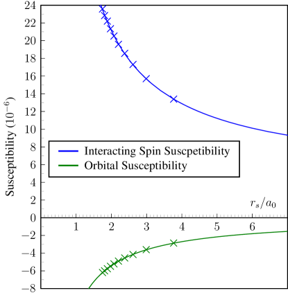
Figure 1: Spin and Orbital susceptibility per unit volume of the interacting-electron homogeneous gas respect to $r_{s}/a_{0}=(3/4\pi\rho)^{3}$. Solid lines represent analytical results while dots represent results computed with this code at $0.4$ eV smearing. The susceptibilities are dimensionless. The exchange-correlation is modeled with the PBE functional.

VIII Simple metals

The object of the present work is to build a quantitative method for computing NMR shifts in metallic compounds. As such, we now study three simple metals: bulk aluminum, bulk lithium, and bulk copper.

Experimentally, NMR shifts are obtained with respect to the response of so-called zero-shift compounds. We will first study this aspect of the problem, and compute the shielding of these compounds. We will then give the computational details for each metal, and finally examine the NMR shifts and macroscopic magnetic susceptibilities.

VIII.1 Computational Details

Computational details are reported in tables 1. For all calculations, we use the Marzari-Vanderbilt smearing functionMarzari et al. (1999) and Troullier-MartinsTroullier and Martins (1991) norm-conserving pseudopotentials. Following experimental conventions, we use a spherical sample when accounting for surface currents. We use the PBEPerdew et al. (1996) exchange-correlation functional.

Aluminum and copper are cubic face centered metals with $a=4.05$ Å and $a=3.61$ Å, respectively. Lithium is body centered with $a=3.49$ Å. We use experimental cell parameters as given by Ref. Ashcroft and Mermin, 1976.

Metal	Smearing	Cutoff		$N_{k}$
		Knight	Orbital	Knight	Orbital
Al	0.15	15	15	29820	62790
Li	0.2	15	15	8094	11900
Cu	0.2	75	90	1300	5740

Table 1: Computational Details. Smearings are given in eV. Plane wave cutoffs for both Knight and orbital shift calculations are given in Rydberg. $N_{k}$ stands for the number of independent ${\bm{\mathrm{k}}}$-points in the irreducible wedge of the Brillouin zone. The Brillouin zone is represented with a discrete Monkhorst-Pack gridMonkhorst and Pack (1976). The Marzari-Vanderbilt smearing functionMarzari et al. (1999) is used.

VIII.2 Zero shift compounds

Experimental NMR shifts are obtained as

$${\bm{\mathrm{u}}}\cdot\tensor{\delta}\cdot{\bm{\mathrm{u}}}=-{\bm{\mathrm{u}}}\cdot(\tensor{\sigma}-\tensor{\sigma}_{ref})\cdot{\bm{\mathrm{u}}},$$ (58)

where ${\bm{\mathrm{u}}}$ is the direction in which the external magnetic field is applied, $\tensor{\sigma}$ is the the shielding of the compound, and $\tensor{\sigma}_{ref}$ is the shielding of the zero-shift compound.

Rather than evaluating $\tensor{\sigma}_{ref}$ directly, we will compute the shielding of some compound for which the NMR shift is well known experimentally, and then deduce $\tensor{\sigma}_{ref}$ from Eq. 58.

Atom	“zero-shift compound”	compound			$\sigma^{ref}$
		type	$\sigma^{th}$	$\delta_{exp}$
Al	AlCl3 in heavy water	AlPO4	519	45	564
Li	aqueous LiCl	Li2O	86	10	96
Cu	CuBr powder	CuBr	424	0.0	424

Table 2: Reference shifts $\sigma^{ref}$. The “compound” columns gives the solid which is used to obtain the reference shift, its calculated isotropic shielding $\sigma^{th}$, and its experimental isotropic shift $\delta_{exp}$. The reference shift is obtained using the relationship $\delta_{exp}=-(\sigma^{th}-\sigma^{ref})$. Shieldings are converged to better than a ppm. Shieldings and shifts are given in ppm.

The reference shifts for each element Al, Li, and Cu are given in Tab. 2. Note that all references are computed on insulators, and hence that the shieldings result only from the orbital response. The latter are computed using the method for insulators described in Ref. Pickard and Mauri, 2001.

VIII.3 Behavior with respect to smearing

The computation of NMR shifts requires a very fine description of the Fermi surface. Hence, one must take care that the computed shifts are indeed converged with respect to smearing. Figures 2 and 3 report the convergence behavior with respect to smearing of, respectively, the spin macroscopic spin-susceptibility, and of the macroscopic orbital-susceptibilities for Aluminum, Lithium, and Copper. Figures 4 and 5 report the behavior of the Knight shift and of the orbital shift, excluding the contribution of the macroscopic susceptibility. We find that the orbital susceptibility is the hardest to converge. This is coherent with the fact that as a second order derivative of the total energy, it depends on very fine details of the Fermi surface. On the other hand, the spin susceptibility is obtained as the average over the unit cell of the spin density. As such, it is comparatively insensitive to details of the Fermi surface, and converges much faster with respect to the smearing parameter. A similar hierarchy is obtained for the convergence behavior of the Knight and orbital shifts (not including their respective susceptibility). It should be noted that in the examples provided here, the Knight shift is by far the largest component of the total NMR shifts. Overall, we expect the total NMR shielding to be converged to better than $4\%$ with respect to smearing and ${\bm{\mathrm{k}}}$-point density.

On the other hand, convergence of the magnetic susceptibility can prove quite arduous. For instance, the orbital susceptibility of Aluminum varies from $-0.3$ to $+5.6$ $10^{-6}$ cm³ mol^-1 within the temperature range 0.3 eV to 0.1 eV. Aluminum presents the slowest convergence of the three metals studied in this work.

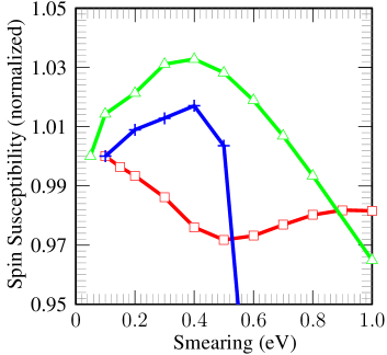
Figure 2: Convergence with respect to smearing ($\sigma$) of the spin susceptibility of Aluminum (green triangles), Lithium (red squares), and Copper (blue +). For comparison purposes, the spin susceptibility of each metal is normalized to its value at the lowest achieved smearing. The $x$-axis represents smearing in eV.

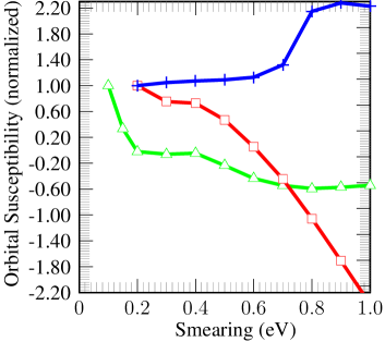
Figure 3: Convergence with respect to smearing ($\sigma$) of the orbital susceptibility of Aluminum (green triangles), Lithium (red squares), and Copper (blue +). For comparison purposes, the orbital susceptibility of each metal is normalized to its value at the lowest achieved smearing. The $x$-axis represents smearing in eV.

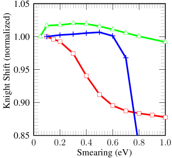
Figure 4: Convergence with respect to smearing ($\sigma$) of the Knight shift (not including the spin susceptibility) of Aluminum (green triangles), Lithium (red squares), and Copper (blue +). For comparison purposes, the Knight shift of each metal is normalized to its value at the lowest achieved smearing. The $x$-axis represents smearing in eV.

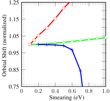
Figure 5: Convergence with respect to smearing ($\sigma$) of the orbital shift (not including the orbital susceptibility) of Aluminum (green triangles), Lithium (red squares), and Copper (blue +). For comparison purposes, the orbital shift of each metal is normalized to its value at the lowest achieved smearing. The $x$-axis represents smearing in eV.

VIII.4 Results and Discussion

VIII.4.1 Macroscopic Magnetic Susceptibility

The computed magnetic susceptibility are referenced in Tab. 3. Overall, agreement is very good. It contains a diamagnetic contribution from the core electrons. This contribution is constant within the frozen core approximation and is computed once and for all from an atomic code for each pseudo-potential. Tab. 4 compares the spin and orbital susceptibilities of each metal to an electronic gas of corresponding mean density.

When examining the band structure of Aluminum, one finds that it is quite similar to that of an homogeneous gas of equivalent density. As a result, the non-interacting spin susceptibility and the Stoner factor of these two systems are remarkably close. This indicates that not only are their density of states at the Fermi level similar, but also the Pauli-mediated behavior of the electrons with respect to a pertubation of the spin population. On the other hand, the orbital susceptibility of these two systems are quite different (note however that for Aluminum, we did not achieve good convergence of this quantity with respect to smearing). Indeed, in an ideal gas, the contribution of lower lying electrons cancels-out exactly. Thus, only electrons at the Fermi level contribute to the orbital susceptibility. This is usually not true in more complex systems. Even small differences between the band structures of Aluminum and the homogeneous gas will result in appreciably different orbital susceptibilities.

Lithium presents a case very different from the one above. Its non-interacting spin susceptibility is much larger than that of the homogeneous gas. As a result, the large polarization at the Fermi level yields a large polarization of the lower-lying electronic wavefunctions. The Stoner factor of Lithium is much larger than that of the homogeneous electron gas. Interestingly, Lithium presents very little orbital susceptibility.

Copper presents a different picture still. Indeed, it has a rather low density of states at the Fermi level compared to the homogeneous gas. As a result, both non-interacting and interacting spin-susceptibilities are small. On the other hand, the large number of lower lying electrons, including $d$ electrons, yield an appreciable diamagnetic orbital susceptibility. As such, of the three metals studied here, it is the only one with a diamagnetic susceptibility. It is worthwhile to note that only the orbital susceptibility can explain such a behavior, and that hence a complete understanding of the susceptibility of Copper requires the computation of both spin and orbital contributions.

Metal	$\chi_{s}$		$\chi_{o}$		$\chi_{core}$	$\chi^{th}$	Exp.
Al	17.7 $\pm$	0.2	1.9 $\pm$	5	-3.0	16.6	16.5 [Carter et al., 1977]
Li	28.4 $\pm$	0.5	0.7 $\pm$	1	-0.7	28.4	24.5$\pm 0.3$ [Dugan, 1997]
Cu	10.8 $\pm$	0.2	-13.1 $\pm$	1	-4.5	-6.8	-5.3 [Bowers, 1956]

Table 3: Isotropic magnetic macroscopic susceptibility (in $10^{-6}$  cm ³ mol^-1, moles of atoms). The susceptibility contains three components: (i) the orbital susceptibility ($\chi_{o}$), (ii) the spin susceptibility ($\chi_{s}$), and (iii) the diamagnetic susceptibility of the core electrons ($\chi_{core}$). As shown in Fig. 3, we were unable to converge the orbital susceptibility of Aluminum.

System	$\chi_{s}^{0}$	Stoner	$\chi_{s}$	$\chi_{o}$
Al	13.2	1.34	17.7	1.9
gas	12.5	1.31	16.4	-4.2
Li	15.5	1.83	28.4	0.7
gas	10.2	1.48	15.1	-3.4
Cu	9.5	1.14	10.8	-13.1
gas	15.3	1.18	18.1	-5.1

Table 4: Isotropic magnetic macroscopic susceptibilities (in $10^{-6}$  cm ³ mol^-1, moles of atoms). $\chi_{s}^{0}$ is the non-interacting spin susceptibility, $\chi_{s}$ the interacting spin susceptibility, and $\chi_{o}$ the orbital susceptibility. For comparison, the susceptibilities of a homogeneous gas of the same mean density as the system is given.

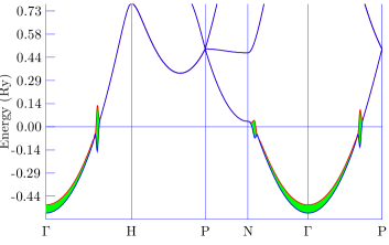
Figure 6: Band structure of lithium. The width of the line is representative of its contribution to the isotropic Knight shift. The Fermi energy is set to zero on the energy scale. Computations were done with a smearing of 0.2 eV, for which the $\frac{1}{T}$ dependence is obvious at the Fermi energy. The ”divergence” in $T$ disappears with the Brillouin zone integration.

VIII.4.2 NMR shifts

The computed isotropic NMR shifts are reported in Tab. 5. Tab. 6 also report $\sigma_{s}/\sigma_{s}^{0}$, a quantity akin to the Stoner factor of the susceptibility, where $\sigma_{s}$ is the Knight shift computed including self-consistency, and $\sigma_{s}^{0}$ the Knight shift computed without self-consistency.

The NMR shift of Aluminum results predominantly from the Knight shift. It is worthwhile to note that the orbital and Knight shielding tensors are of similar magnitude, $-548$ ppm and $1862$ ppm respectively. Yet, whereas the Knight contribution enters into the NMR shift as a whole, the orbital part enters as a variation of the absolute orbital shielding tensor between pure Al and ionic Al (which presents no Knight shift), yielding a much smaller contribution. Previous theoretical calculationsMishra et al. (1990) predict a Knight shielding of $\sigma_{s}=1707$ ppm. Although, the authors of Ref. Mishra et al., 1990 do not compute NMR shifts comparable to experiment, in the sense that they do not reference their results to a computed zero-shift compound, their result is close to experimental value because of the predominance of the Knight shift. As will be the case for the other metals studied here, the ratio $\sigma_{s}/\sigma_{s}^{0}$ and the Stoner factor are quite close in value. Indeed, both quantities represent the same physical phenomena, namely the interplay between the Kohn-Sham potential of the valence electrons and the spin polarization at the Fermi level.

Again, the orbital shift of Lithium is by far smaller than its Knight shift. As mentioned previously, the lower lying levels are heavily polarized by electrons at the Fermi surface. The authors of Ref. Gaspari et al., 1964 estimated the Knight shift of Lithium including core-polarization. Even in this case, where from Fig. 6 one would expect a rather high polarization, the contribution is only of the order of 5% of the whole (250 ppm). More recently Mishra et al estimate a Knight shift of 301.9 ppmMishra et al. (1990). Overall, our calculation agrees very well with experimental values. The ratio $\sigma_{s}/\sigma_{s}^{0}$ is relatively smaller than the Stoner factor. One should note that the latter is a ratio of the average spin-polarization over the whole unit cell, whereas the former is the ratio over the spin-polarization at a single point of unit cell, namely the position of the Lithium nucleus. The discrepancy between the two quantities implies simply that the effect of the spin polarization is smaller at the nucleus than on average across the cell.

Of the three metals studied here, Copper is the only one which presents an appreciable orbital contribution to the NMR shift. It is probably a result of the filled $d$-bands. Nonetheless, as large as the orbital contribution may be, the Knight shift is larger still. Interestingly, the computed absolute orbital shielding tensor (including both valence and core contributions) is rather small (26 ppm). It would seem that a substantial paramagnetic contribution from the valence electrons cancels out the substantial diamagnetic contribution from the core electrons (computed to be 2171 ppm). In other words, whereas in Li and Al, the reference compound and the metals had similar orbital shielding tensor, the orbital behavior of metallic Cu is very different from that of Copper-Bromide. As was the case for the magnetic spin susceptibility, the spin-polarization at the Fermi level has little effect on the lower lying levels, resulting in a relatively small $\sigma_{s}/\sigma_{s}^{0}$ ratio and Stoner factor.

Metal	$\sigma_{s}$		$\sigma_{o}-\sigma_{ref}$		$\delta$	Exp.
Al	-1858 $\pm$	70	-16 $\pm$	8	1874	1640 [Sagalyn and Hofmann, 1962],
Li	-266 $\pm$	5	-15 $\pm$	1	281	260 [Carter et al., 1977]
Cu	-2336 $\pm$	20	-450 $\pm$	10	2786	2380 [Carter et al., 1977],

Table 5: Isotropic NMR shifts of a few simple metals. For comparison, the orbital shielding with respect to the reference and the Knight shifts are given as well. The isotropic NMR shifts are given by the relationship $\delta=-(\sigma_{o}+\sigma_{s}-\sigma_{ref})$. Estimates of the convergence with respect to temperature and Brillouin zone sampling are given in the first two columns.

Metal	$\sigma_{s}^{0}$	$\sigma_{s}/\sigma_{s}^{0}$	$\sigma_{s}$	$\sigma_{o}-\sigma_{ref}$	$\delta$	Exp.
Al	-1330	1.40	-1858	-16	1874	1640 [Sagalyn and Hofmann, 1962],
Li	-157	1.69	-266	-15	281	260 [Carter et al., 1977]
Cu	-2121	1.10	-2336	-604	2940	2380 [Carter et al., 1977],

Table 6: Isotropic NMR shifts of a few simple metals. $\sigma_{s}^{0}$ is the non-interacting Knight shift computed without the self-consistent part of the pertubation. The ratio $\sigma_{s}/\sigma_{s}^{0}$ is the Knight shift equivalent of Stoner factor of the spin susceptibility. Unsurprisingly, this ratio is quite close to the Stoner factor. Indeed both are a measure of the interplay between the spin-polarization at the Fermi level and lower-lying valence electrons.

IX Conclusions

We have presented a unified method for computing NMR shifts in metals. Our approach yields shifts which are directly comparable to experimental data, in the sense that both orbital and Knight shifts are computed. It was implemented within a pseudo-potential, plane-wave density functional theory code. All-electron quantities were recovered using the PAW approach. Gauge invariance was enforced with GIPAW. We compared results given by our approach to known analytical solutions for the homogeneous gas. Finally we successfully computed the NMR shifts of simple metals, with good comparison to experimental results. In conclusion, we have described a method which can accurately recover the NMR shifts of real metallic systems, thus allowing a better interpretation of NMR data. Next, we expect to study semi-metallic systems, such as graphite and nanotubes, for which an accurate description of both orbital and Knight shift is of paramount importance.

Appendix A The Generalized $f$-sum rule

Let $\mathcal{O}$ and $\mathcal{E}$ be odd and even operators respectively on time reversal, i.e. for any real wave-functions ${|\Psi\rangle}$ and ${|\Psi^{\prime}\rangle}$:

$$\langle\Psi|\mathcal{O}{|\Psi^{\prime}\rangle}=-\langle\Psi^{\prime}|\mathcal{O}{|\Psi\rangle},\quad\langle\Psi|\mathcal{E}{|\Psi^{\prime}\rangle}=\langle\Psi^{\prime}|\mathcal{E}{|\Psi\rangle}$$ (59)

Let ${|\Psi_{i}\rangle}$ be the eigen-wave-functions of the hamiltonian $\mathcal{H}$, with eigenvalues $\epsilon_{i}$. Let $f(x)$ be a smearing function and $\sigma$ the smearing. Then the occupation factors are defined as $f_{j,i}=f(\frac{\epsilon_{j}-\epsilon_{i}}{\sigma})$ (where $i,j=F$ stands for the Fermi energy $\epsilon_{F}$, and finally, let

$$s=\sum_{i}\ \Re\left\{\langle\Psi_{i}|\mathcal{O}\ \mathcal{G}(\epsilon_{i})\ \frac{1}{\imath}\left[\mathcal{E},\mathcal{H}\right]{|\Psi_{i}\rangle}\right\}\$$ (60)

$$\mathcal{G}(\epsilon_{i})=\sum_{j}\frac{f_{F,j}-f_{F,i}}{\epsilon_{j}-\epsilon_{i}}{|\Psi_{j}\rangle}\langle\Psi_{j}|$$ (61)

where $\Re$ is the real part. Then, using the fact that $\mathcal{H}{|\Psi_{i}\rangle}=\epsilon_{i}{|\Psi_{i}\rangle}$, we arrive at the expression:

$$s=-\sum_{i,j}\left(f_{F,j}-f_{F,i}\right)\ \Re\left[\langle\Psi_{i}|\mathcal{O}{|\Psi_{j}\rangle}\langle\Psi_{j}|\frac{1}{\imath}\mathcal{E}{|\Psi_{i}\rangle}\right]$$ (62)

which can be separated into two sums:

$$s=\sum_{i,j}f_{F,i}\Re\left[\langle\Psi_{i}|\mathcal{O}{|\Psi_{j}\rangle}\langle\Psi_{j}|\frac{1}{\imath}\mathcal{E}{|\Psi_{i}\rangle}\right]\\ -\sum_{i,j}f_{F,j}\Re\left[\langle\Psi_{i}|\mathcal{O}{|\Psi_{j}\rangle}\langle\Psi_{j}|\frac{1}{\imath}\mathcal{E}{|\Psi_{i}\rangle}\right]$$ (63)

Swapping dummy indexes in the second term:

$$s=\sum_{i,j}f_{F,i}\Re\left[\langle\Psi_{i}|\mathcal{O}{|\Psi_{j}\rangle}\langle\Psi_{j}|\frac{1}{\imath}\mathcal{E}{|\Psi_{i}\rangle}\right]\\ -\sum_{i,j}f_{F,\imath}\Re\left[\langle\Psi_{j}|\mathcal{O}{|\Psi_{j}\rangle}\langle\Psi_{i}|\frac{1}{\imath}\mathcal{E}{|\Psi_{j}\rangle}\right]$$ (64)

Then, using the parity of $\mathcal{O}$ and $\mathcal{E}$:

$$s=\sum_{i,j}f_{F,i}\Re\left[\langle\Psi_{i}|\mathcal{O}{|\Psi_{j}\rangle}\langle\Psi_{j}|\frac{1}{\imath}\mathcal{E}{|\Psi_{i}\rangle}\right]\\ +\sum_{i,j}f_{F,i}\Re\left[\langle\Psi_{i}|\mathcal{O}{|\Psi_{j}\rangle}\langle\Psi_{j}|\frac{1}{\imath}\mathcal{E}{|\Psi_{i}\rangle}\right]$$ (65)

After remarking that $\sum_{j}{|\Psi_{j}\rangle}\langle\Psi_{j}|=1$:

$$s=2\sum_{i}f_{F,i}\Re\left[\langle\Psi_{i}|\frac{1}{\imath}\mathcal{O}\mathcal{E}{|\Psi_{i}\rangle}\right]$$ (66)

Expanding the real value, we arrive at the result:

$$-\sum_{i}\ \Re\left\{\langle\Psi_{i}|\mathcal{O}\ \mathcal{G}(\epsilon_{i})\ \frac{1}{\imath}\left[\mathcal{E},\mathcal{H}\right]{|\Psi_{i}\rangle}\right\}\ =\\ \sum_{i}f_{F,i}\langle\Psi_{i}|\frac{1}{\imath}\left[\mathcal{E},\mathcal{O}\right]{|\Psi_{i}\rangle}$$ (67)

Expression 67 and equation (A7) in the appendix of Ref. Pickard and Mauri, 2001 differ by the definition of the Green function and the range of the sum over states. At zero temperature and in insulators, the results are equivalent.

References

• Grant and Harris (1996) D. M. Grant and R. K. Harris, eds., The Encyclopedia of NMR (Wiley, London, 1996).
• Pines (1997) D. Pines, Z. Phys. B 103, 129 (1997).
• Keith and Bader (1992) T. A. Keith and R. F. W. Bader, Chem. Phys. Lett. 194, 1 (1992).
• Pickard and Mauri (2001) C. J. Pickard and F. Mauri, Phys. Rev. B: Condens. Matter 63, 245101 (2001).
• Sebastiani and Parrinello (2001) D. Sebastiani and M. Parrinello, J. Phys. Chem. A 105, 1951 (2001).
• Profeta et al. (2003) M. Profeta, F. Mauri, and C. J. Pickard, J. Am. Chem. Soc. 125, 541 (2003).
• Umari and Pasquarello (2005) P. Umari and A. Pasquarello, Phys. Rev. Lett. 95, 137401 (2005).
• Tripathi et al. (1981) G. S. Tripathi, L. K. Das, , P. K. Misra, and S. D. Mahanti, Solid State Commun. 38, 1207 (1981).
• Pavarini and Mazin (2001) E. Pavarini and I. I. Mazin, Phys. Rev. B: Condens. Matter 64, 140504 (2001).
• Lauginie et al. (1988) P. Lauginie, H. Estrade-Szwarckopf, B. Rousseau, and J. Conard, CR. Acad. Sci. Paris 307II, 1693 (1988).
• Hiroyama and Kume (1988) Y. Hiroyama and K. Kume, Solid State Commun. 65, 617 (1988).
• Lauginie et al. (1993) P. Lauginie, A. Messaoudi, and J. Conard, Synthetic Metals 56, 3002 (1993).
• Kobayashi and Tsukada (1988) K. Kobayashi and M. Tsukada, Phys. Rev. B: Condens. Matter 38, 8566 (1988).
• Ajiki and Ando (1995) H. Ajiki and T. Ando, J. Phys. Soc. Japan 64, 4382 (1995).
• Stokes et al. (1982a) H. T. Stokes, H. E. Rhodes, P.-K. Wang, C. P. Slichter, and J. H. Sinfelt, Phys. Rev. B: Condens. Matter 26, 3559 (1982a).
• Stokes et al. (1982b) H. T. Stokes, H. E. Rhodes, P.-K. Wang, C. P. Slichter, and J. H. Sinfelt, Phys. Rev. B: Condens. Matter 26, 3575 (1982b).
• Makowka et al. (1985) C. D. Makowka, C. P. Slichter, and J. H. Sinfelt, Phys. Rev. B: Condens. Matter 31, 5663 (1985).
• Vuissoz et al. (1999) P.-A. Vuissoz, J.-P. Ansermet, and A. Wieckowski, Phys. Rev. B: Condens. Matter 83, 2457 (1999).
• Blöchl (1994) P. E. Blöchl, Phys. Rev. B: Condens. Matter 50, 17953 (1994).
• de Gironcoli (1995) S. de Gironcoli, Phys. Rev. B: Condens. Matter 51, 6773 (1995).
• van de Walle and Blöchl (1993) C. G. van de Walle and P. E. Blöchl, Phys. Rev. B: Condens. Matter 47, 4244 (1993).
• Pacchioni et al. (2000) G. Pacchioni, F. Frigoli, D. Ricci, and J. A. Weil, Phys. Rev. B: Condens. Matter 63, 54102 (2000).
• Ashcroft and Mermin (1976) N. W. Ashcroft and N. D. Mermin, Solid State Physics (Brooks/Cole, 1976).
• Perdew et al. (1996) J. P. Perdew, K. Burke, and M. Ernzerhof, Phys. Rev. Lett. 77, 3865 (1996).
• Marzari et al. (1999) N. Marzari, D. Vanderbilt, A. De Vita, and M. C. Payne, Phys. Rev. Lett. 82, 3296 (1999).
• Troullier and Martins (1991) N. Troullier and J. L. Martins, Phys. Rev. B: Condens. Matter 43, 1993 (1991).
• Monkhorst and Pack (1976) H. J. Monkhorst and J. D. Pack, Phys. Rev. B: Condens. Matter 13, 5188 (1976).
• Carter et al. (1977) G. C. Carter, L. H. Benett, and D. J. Kahan, Progress in Material Science 20, 1 (1977).
• Dugan (1997) D. Dugan, Phys. Rev. B: Condens. Matter 57, 7759 (1997).
• Bowers (1956) R. Bowers, Phys. Rev. 102, 1486 (1956).
• Mishra et al. (1990) B. Mishra, L. K. Das, T. Sahu, G. S. Tripathi, and P. K. Misra, J Phys. : Cond. Mat. 2, 9891 (1990).
• Gaspari et al. (1964) G. D. Gaspari, W. Shyu, and T. P. Das, Phys. Rev. 134, A852 (1964).
• Sagalyn and Hofmann (1962) P. L. Sagalyn and J. A. Hofmann, Phys. Rev. 127, 68 (1962).