Data Mining-based Materialized View and Index Selection
in Data Warehouses

Abstract

Materialized views and indexes are physical structures for accelerating data access that are casually used in data warehouses. However, these data structures generate some maintenance overhead. They also share the same storage space. Most existing studies about materialized view and index selection consider these structures separately. In this paper, we adopt the opposite stance and couple materialized view and index selection to take view-index interactions into account and achieve efficient storage space sharing. Candidate materialized views and indexes are selected through a data mining process. We also exploit cost models that evaluate the respective benefit of indexing and view materialization, and help select a relevant configuration of indexes and materialized views among the candidates. Experimental results show that our strategy performs better than an independent selection of materialized views and indexes.

Keywords: Data warehouses, Performance optimization, Materialized views, Indexes, Data mining, Cost models.

1 Introduction

Large-scale usage of databases in general and data warehouses in particular requires an administrator whose principal role is data management, both at the logical level (schema definition) and physical level (files and disk storage), as well as performance optimization. With the wide development of Database Management Systems (DBMSs), minimizing the administration function has become crucial ( ?). One important administration task is the selection of suitable physical structures to improve system performance by minimizing data access time ( ?).

Among techniques adopted in data warehouse relational implementations for improving query performance, view materialization and indexing are presumably the most effective ( ?). Materialized views are physical structures that improve data access time by precomputing intermediary results. Therefore, end-user queries can be efficiently processed through data stored in views and do not need to access the original data. Indexes are also physical structures that allow direct data access. They avoid sequential scans and thereby reduce query response time. Nevertheless, exploiting either materialized views or indexes requires additional storage space and entails maintenance overhead when refreshing the data warehouse. The issue is thus to select an appropriate configuration (set) of materialized views and indexes that minimizes query response time and the selected data structures’ maintenance cost, given a limited storage space.

The literature regarding materialized view and index selection in relational databases and data warehouses is quite abundant. However, we have identified two key issues requiring enhancements. First, the actual selection of suitable candidate materialized views and indexes is rarely addressed in existing approaches. Most of them indeed present scaling problems at this level. Second, none of these approaches takes into account the interactions that may exist between materialized views, between indexes, and between indexes and materialized views (including the approaches that simultaneously select both materialized views and indexes).

In this paper, we present a novel strategy for optimizing data warehouse performance that aims at addressing both these issues. We have indeed designed a generic approach whose objective is to automatically propose solutions to data warehouse administrators for optimizing data access time. The principle of this approach is to apply data mining techniques on a workload (set of queries) that is representative of data warehouse usage in order to deduce a quasi-optimal configuration of materialized views and/or indexes. Data mining actually helps reduce the selection problem’s complexity and improves scalability. Then, cost models help select among the selected materialized views and indexes the most efficient in terms of performance gain/overhead ratio. We have applied our approach on three related problems: isolate materialized view selection, isolate index selection and joint materialized view and index selection. In the last case, we included index-view interactions in our cost models.

The remainder of this paper is organized as follows. Section 2 presents and discusses the state of the art regarding materialized view and index selection. Section 3 motivates and presents the principle of our performance optimization approach. Section 4 further details how we apply this approach to isolate materialized view selection, isolate index selection and joint materialized view and index selection, respectively. We particularly focus on joint materialized view and index selection, which is our latest development. Section 5 presents the experimental results we achieved to illustrate our approach’s relevance. Finally, we conclude this paper and provide research perspectives in Section 6.

2 Related work

In this section, we first formalize the materialized view and index selection problem, and then detail and discuss the state of the art regarding materialized view selection, index selection and joint index and materialized view selection, respectively.

2.1 Materialized view and index selection: formal problem definition

The materialized view and index selection problem consists in building a set of materialized views and indexes that optimizes the execution cost of a given workload. This optimization may be realized under constraints, typically the storage space available for storing these physical data structures.

Let $V_{C}$ and $I_{C}$ be two sets of materialized views and indexes, respectively, that are termed candidate and are susceptible to reduce the execution cost of a given query set $Q$ (generally supposed representative of system workload). Let $O_{C}=V_{C}\cup I_{C}$. Let $S$ be the storage space allotted by the data warehouse administrator to build objects (materialized views or indexes) from set $O_{C}$. The joint materialized view and index selection problem consists in building an object configuration $O\subseteq O_{C}$ that minimizes the execution cost of $Q$, under storage space constraint. This NP-hard problem ( ?, ?) may be formalized as follows:

• $cost(Q,O)=min(cost(Q,\vartheta))~{}\forall~{}\vartheta\subseteq O_{C}$ ;

• $\displaystyle{\sum_{o\in O}}size(o)\leq S$, where $size(o)$ is the disk space occupied by object $o$.

2.2 Materialized view selection

The materialized view selection problem has received significant attention in the literature. Related researches differ in several points:

1. the way the set of candidate views $V_{C}$ is determined;

2. the framework used to capture relationships between candidate views;

3. the use of mathematical cost models vs. calls to the system’s query optimizer;

4. view selection in the relational or multidimensional context;

5. multiple or simple query optimization;

6. theoretical or technical solutions.

Classical papers in materialized view selection introduce a lattice framework that models and captures dependency (ancestor or descendent) among aggregate views in a multidimensional context ( ?, ?, ?, ?). This lattice is greedily browsed with the help of cost models to select the best views to materialize. This problem has first been addressed in one data cube and then extended to multiple cubes ( ?). Another theoretical framework, the AND-OR view graph, may also be used to capture the relationships between views ( ?, ?, ?, ?). Unfortunately, the majority of these solutions are theoretical and are not truly scalable.

A wavelet framework for adaptively representing multidimensional data cubes has also been proposed ( ?). This method decomposes data cubes into an indexed hierarchy of wavelet view elements that correspond to partial and residual aggregations of data cubes. An algorithm greedily selects a non-expensive set of wavelet view elements that minimizes the average processing cost of data cube queries. In the same spirit, ? (?) proposed the Dwarf structure, which compresses data cubes. Dwarf identifies prefix and suffix redundancies within cube cells and factors them out by coalescing their storage. Suppressing redundancy improves the maintenance and interrogation costs of data cubes. These approaches are very interesting, but they are mainly focused on computing efficient data cubes by changing their physical design.

Other approaches detect common sub-expressions within workload queries in the relational context ( ?, ?, ?). The view selection problem then consists in finding common subexpressions corresponding to intermediary results that are suitable to materialize. However, browsing is very costly and these methods are not truly scalable with respect to the number of queries.

Finally, the most recent approaches are workload-driven. They syntactically analyze a workload to enumerate relevant candidate views ( ?). By exploiting the system’s query optimizer, they greedily build a configuration of the most pertinent views. A workload is indeed a good starting point to predict future queries because these queries are probably within or syntactically close to a previous query workload. In addition, extracting candidate views from the workload ensures that future materialized views will probably be used when processing queries.

2.3 Index selection

The index selection problem has been studied for many years in databases ( ?, ?, ?, ?, ?, ?, ?). In the more specific context of data warehouses, existing research studies may be clustered into two families: algorithms that optimize maintenance cost ( ?) and algorithms that optimize query response time ( ?, ?, ?). In both cases, optimization is realized under storage space constraint. In this paper, we focus on the second family of solutions, which is relevant in our context. Studies falling in this category may be further categorized depending on how the set of candidate indexes $I_{C}$ and the final configuration of indexes $I$ are built.

Selecting a set of candidate indexes may be automatic or manual. Warehouse administrators may indeed appeal to their expertise and manually provide, from a given workload, a set of candidate indexes ( ?, ?, ?). Such a choice is however subjective. Moreover, the task may be very hard to achieve when the number of queries is very high. In opposition, candidate indexes can also be extracted automatically, through a syntactic analysis of queries ( ?, ?, ?). Such an analysis depends on the DBMS, since each DBMS is queried through a specific syntax derived from the SQL standard.

The methods for building a final index configuration from candidate indexes may be categorized into:

1. ascending or descending greedy methods;

2. methods derived from genetic algorithms;

3. methods assimilating the selection problem to the well-known knapsack optimization problem.

Ascending greedy methods start from an empty set of candidate indexes ( ?, ?, ?, ?). They incrementally add in indexes minimizing cost. This process stops when cost ceases decreasing. Contrarily, descending greedy methods consider the whole set of candidate indexes as a starting point. Then, at each iteration, indexes are pruned ( ?, ?). If workload cost before pruning is lower (respectively, greater) than workload cost after pruning, the pruned indexes are useless (respectively, useful) for reducing cost. The pruning process stops when cost increases after pruning.

Genetic algorithms are commonly used to resolve optimization problems. They have been adapted to the index selection problem ( ?). The initial population is a set of input indexes (an index is assimilated to an individual). The objective function to optimize is the workload cost corresponding to an index configuration. The combinatory construction of an index configuration is realized through the crossover, mutation and selection genetic operators. Eventually, the index selection problem has also been formulated in several studies as a knapsack problem ( ?, ?, ?, ?) where indexes are objects, index storage costs represent object weights, workload cost is the benefit function, and storage space is knapsack size.

2.4 Joint materialized view and index selection

Few research studies deal with simultaneous index and materialized view selection. ? (?) have proposed three strategies. The first one, MVFIRST, selects materialized views first, and then indexes, taking the presence of selected views into account. The second alternative, INDFIRST, selects indexes first, and then materialized views. The third alternative, joint enumeration, processes indexes, materialized views and indexes over these views at the same time. According to the authors, this approach is more efficient than MVFIRST and INDFIRST, but no further details are provided.

? (?) studied storage space distribution among materialized views and indexes. First, a set of materialized views and indexes is designed as an initial solution. Then, the approach iteratively reconsiders the solution to further reduce execution cost, by redistributing storage space between indexes and materialized views. Two agents are in perpetual competition: the index spy (respectively, view spy) steals some space allotted to materialized views (respectively, indexes), and vice versa. The recovered space is used to create new indexes (respectively, materialized views) and prune views (respectively, indexes), according to predefined replacement policies.

Another approach a priori determines a trade-off between storage space allotted to indexes and materialized views, depending on query definition ( ?). According to the authors, the key factors to leverage query optimization is aggregation level, defined by the attribute list of Group by clauses in SQL queries, and the selectivity of attributes present in Where and Having clauses. View materialization indeed provides a great benefit for queries involving coarse granularity aggregations (few attributes in the Group by clause) because they produce few groups among a large number of tuples. On the other hand, indexes provide their best benefit with queries containing high selectivity attributes. Thus, queries with fine aggregations and high selectivity stimulate indexing, while queries with coarse aggregations and weak selectivity encourage view materialization.

Finally, ? (?) have recently worked on refining the physical design of relational databases. Their objective was to automatically improve an expert’s physical design, to take into account primordial constraints it might violate. Hence, they proposed a transformation architecture base on two fusion and reduction primitives that helps process indexes and materialized views in a unified way.

2.5 Discussion

Existing studies related to index and materialized view selection are numerous and diverse in the field of databases, and quite developed in the field of data warehouses as well. However, we have identified two main points that could be improved in these approaches.

2.5.1 Candidate object selection

Selecting candidate objects (materialized views and indexes) is rarely the focus of existing approaches, most of which do not scale up well at this level. Many index selection strategies indeed rest on human expertise (the warehouse administrator’s) to propose an initial candidate index configuration. Given the size and complexity of most data warehouses, an automatic approach is mandatory to apply these methods on a real-life scale. The most recent studies actually take this option, by building the initial index configuration from system workload.

With respect to materialized views, various data structures have been proposed (lattices, graphes, wavelets…) to model inter-view relationships. None of them scale up very well. For instance, browsing a candidate view lattice is very costly when the input data cube is very large. Similarly, building view graphs is as complex as the input workload is large. Hence, it is necessary to carefully evaluate a strategy’s complexity before adopting it, and to optimize any data structure used.

2.5.2 Inter-object interaction management

None of the approaches we have presented in this section takes into account the interactions that may exist between indexes, between materialized views, and between index and views, including joint selection methods. Existing studies, especially those assimilating the selection problem to the knapsack problem or exploiting genetic algorithms, indeed compute the cost or benefit of an object (index or materialized view) once only, before injecting it in their algorithm. However, the relevance of selecting a given object may vary from one iteration to the other if another, previously selected object interacts with the first one. It is thus primordial to recompute costs or benefits dynamically before object selection.

The nearest solution is the one by ? (?). However, its object replacement policies in the disk spaces allotted to indexes and materialized views do not truly reflect index-view interactions. They indeed only consider joint usage frequency in queries, and not the benefit an object brings with respect to other objects.

3 Data mining-based warehouse performance optimization approach

In this section, we first motivate our performance optimization approach. Then, we present its general principle, detail how candidate objects are selected and how a final object (materialized view and index) configuration is generated.

3.1 Motivation

In this paper, our objective is to address the issues identified in Section 2.5. First, to ensure that candidate object (materialized view or index) selection scales up, it is necessary to devise an automatic approach. Generally, this is achieved by syntactically analyzing the system’s query workload, which helps identify query attributes that might support indexes or materialized views. These attributes are then systematically combined to propose multi-attribute indexes or exhaustive view graphs. However, this strategy later leads, in the selection phase, to consider irrelevant objets, i.e., objects that do belong to the workload, but are not interesting in the scope of indexing or view materialization.

To a priori eliminate these irrelevant objects, we propose to exploit data mining techniques to directly extract from the workload a configuration of pertinent candidate objects. Our idea is to discover co-occurencies and similarities between workload objects. For indexing, we base our approach on the intuition that the importance of an attribute to index is strongly correlated with its appearance frequency in the workload. For view materialization, devising similar classes of queries also helps build views that are likely to answer all the queries from a given class.

On the basis of the smallest possible set of candidate, all relevant objects, we must then exploit an optimization algorithm (typically a greedy, knapsack or genetic algorithm) to build a quasi-optimal object configuration. However, to take index-view interactions into account, such algorithms must be modified. In a given iteration, an object’s cost indeed depends on previously selected objects. Thus, it must be recomputed at each step. For simplicity reasons, we implemented this approach in a greedy algorithm.

3.2 General principle of our approach

Our automatic warehouse performance optimization approach (Figure 1) is not only based on information extracted from the warehouse’s data (statistics such as attribute selectivity, for instance) or workload, but also on knowledge. This knowledge includes classical warehouse metadata (we notably exploit the database schema), as well as administration expertise, formalized in cost models (benefit induced by an index and maintenance cost, for instance) or rules. Our approach proceeds in two main steps, which are both piloted by knowledge.

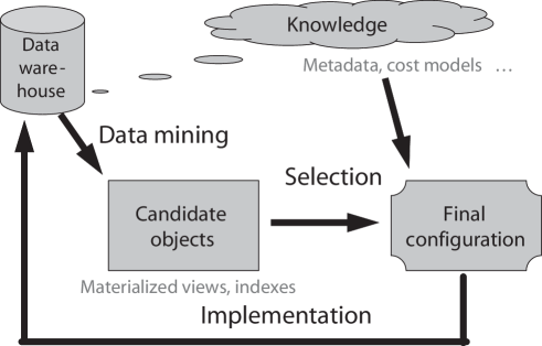
Figure 1: Principle of our automatic performance optimization approach

The first step is building a candidate object configuration $O_{C}$. It consists in syntactically analyzing the input workload, which helps identify attributes that might be useful for view materialization or indexing. Applying rules issued from administration-related knowledge can already reduce the size of this attribute set. For instance, a low selectivity attribute such as gender, which has only two values, is not a good candidate index. This set of attributes is then structured as an attribute-value table that can be processed by a data mining algorithm. The output of such an algorithm is directly the candidate object configuration.

Since disk space is constrained, it would be impossible to exploit all the candidate objects from $O_{C}$. Thus, the second step in our process is greedily selecting a final object configuration $O$ from $O_{C}$. This algorithm exploits cost models we have developed to express, e.g., the benefit brought by a materialized view or an index, as well as their storage and maintenance costs (Section 4). Eventually, the last step in our approach consists in implementing the final object configuration in the data warehouse.

Note that we have designed this approach in a modular fashion, so that it is as generic as possible. Completing the two main steps indeed brought us to perform choices, but other options would be easy to consider. For instance, the data mining technique we selected for building a candidate index configuration is frequent itemset mining, but another study explored clustering instead ( ?). Besides, we have also used clustering for materialized view selection. Similarly, other optimization algorithms could be substituted to the greedy strategy we adopted to build the final object configuration. Our cost models might also be easily replaced with others if necessary, or by calls to a query optimizer, if it is accessible on the host DBMS.

3.3 Candidate object selection

System workload is typically accessible from the host DBMS’ transaction log. A given workload is supposed representative if it has been measured during a time period the warehouse administrator judges sufficient to anticipate upcoming transactions.

Since we are more particularly interested in decision-support query performance and not warehouse maintenance, we only consider interrogation query workloads in this paper. These queries are typically composed of join operations between the fact table and dimensions, restriction predicates and aggregation and grouping operations. More formally, an analytic query $q$ may be expressed as follows in relational algebra: $q=\Pi_{G,M}(\sigma_{R}(F\bowtie D_{1}\bowtie D_{2}\bowtie...\bowtie D_{d}))$, where $G$ is the set of attributes from dimensions $D_{i}$ that are present in $q$’s grouping clause, $M$ is a set of aggregate measures from fact table $F$ and $R$ a conjunction of predicates over dimension attributes.

Attributes that may support materialized views or indexes belong to sets $G$ and $R$ ( ?, ?, ?, ?). We reference them in a so-called “query-attribute” binary matrix whose rows represent workload queries $q_{i}$ and whose columns are representative attributes $a_{j}$. The general term $m_{ij}$ of this matrix is equal to one if attribute $a_{j}$ is present in query $q_{i}$, and to zero otherwise. A simple example of query-attribute matrix based on the workload excerpt from Figure 2 is featured in Table 1.

$q_{1}$	SELECT $F$.$a_{1}$, SUM($F$.$a_{2}$) FROM $F$, $D_{1}$
	WHERE $F$.$a_{1}$ = $D_{1}$.$a_{3}$ AND $D_{1}$.$a_{4}$ < 2000
	GROUP BY $F$.$a_{1}$
$q_{2}$	SELECT $F$.$a_{1}$, $F$.$a_{5}$, AVG($F$.$a_{6}$) FROM $F$, $D_{1}$, $D_{2}$
	WHERE $F$.$a_{1}$ = $D_{1}$.$a_{3}$ AND $F$.$a_{5}$ = $D_{2}$.$a_{7}$ AND $D_{2}$.$a_{8}$ = ’ABC’
	GROUP BY $F$.$a_{1}$, $F$.$a_{5}$
$q_{3}$	SELECT $F$.$a_{1}$, $F$.$a_{9}$, SUM($F$.$a_{2}$) FROM $F$, $D_{1}$, $D_{3}$
	WHERE $F$.$a_{1}$ = $D_{1}$.$a_{3}$ AND $F$.$a_{9}$ = $D_{3}$.$a_{10}$
	GROUP BY $F$.$a_{1}$, $F$.$a_{9}$

Figure 2: Workload excerpt

	$a_{1}$	$a_{3}$	$a_{4}$	$a_{5}$	$a_{7}$	$a_{8}$	$a_{9}$	$a_{10}$
$q_{1}$	1	1	1	0	0	0	0	0
$q_{2}$	1	1	0	1	1	1	0	0
$q_{3}$	1	1	0	0	0	0	1	1

Table 1: Sample query-attribute matrix

This data structure directly corresponds to attribute-value tables that are exploited by data mining algorithms. Here, attributes are queries and values, attributes. Applying a data mining technique onto the query-attribute matrix helps obtain a set of candidate objects (materialized views and indexes) $O_{c}$.

3.4 Final object configuration construction

Our final materialized view and index configuration construction algorithm (Figure 3) is based on an ascending greedy search within the input candidate object set $O_{C}$. It starts from an empty final object configuration $O$, and then adds in it object $o$ from $O_{C}$ that maximizes objective function $f_{O}$, at each iteration. For each object $o\in O_{C}$, the value of $f_{O}(o)$ depends on objects already selected in $O$. Thus, it must be recomputed at each iteration, which helps take view-index interactions into account. The algorithm ends when objective function $f_{O}$ cannot be improved any more, when there are no more candidate objects in $O_{C}$, or when storage space $S$ allocated by the warehouse administrator to materialized views and index is full.

$O=\emptyset$ $s_{O}=0$ Repeat       $o_{max}=\emptyset$       $f_{max}=0$       For each $o\in O_{C}$ do            If $f_{O}(o)>f_{max}$ then                 $o_{max}=o$                 $f_{max}=f_{O}(o)$            End if       End for       If $f_{O}(o_{max})>0$ then            $O=O\cup\{o_{max}\}$            $s_{O}=s_{O}+size(o_{max})$            $O_{C}=O_{C}\setminus\{o_{max}\}$       End if Until $f_{O}(o_{max})\leq 0$ or $O_{C}=\emptyset$ or $s_{O}\geq S$

Figure 3: Final object configuration construction algorithm

For a given workload $Q$ and an object configuration $O$, the objective function $f_{O}$ may generally be expressed as follows: $f_{O}(o)=\alpha_{o}~{}benefit_{O}(o)-\beta_{o}~{}maintenance(o)$. Generally, $benefit_{O}(o)=\frac{cost(Q,O)-cost(Q,O\cup\{o\})}{size(o)}$. However, taking view-index interactions into account complicates this function’s computation (Section 4.3.3).

Cost models developed in Section 4 help compute the $cost$ and $maintenance$ functions. Coefficient $\alpha_{o}$ helps ponder benefit. It is generally equal to one, but may also help favor index that avoid join operations (Section 4.2). Finally, coefficient $\beta_{o}=|Q|p(o)$ is an estimator for the number of updates of object $o$. The update probability of object $o$, $p(o)$, is equal to $\frac{1}{|O|}\frac{\%refreshment}{\%interrogation}$, where $\frac{\%refreshment}{\%interrogation}$ represents the proportion of warehouse updates with respect to interrogations.

4 Applications

This section presents three instances of our automatic data warehouse performance optimization approach: automatic materialized view selection, automatic index selection, and automatic, joint materialized view and index selection. We particularly detail this last, newest application. Moreover, we particularly insist, for each application, on its specificities in terms of candidate object selection (e.g., the data mining technique we exploited) and cost models used in building the final object configuration.

4.1 Clustering-based materialized view selection

In this application, we propose to select materialized views by clustering queries from workload $Q$. Several syntactically similar queries have indeed a high probability of being resolved by one single materialized view. Then, we must build classes of similar queries from $Q$. Since the number of classes is a priori unknown, we have selected an unsupervised clustering method.

Our approach’s principle is similar to SQL workload compression ( ?), a technique proposed in the relational database context to optimize, for instance, index selection or approximate answer to aggregation queries. We adapted this idea to the context of relational (with an SQL decision-support workload) and XML (with an XQuery decision-support workload) data warehouses ( ?, ?).

The main improvement brought by our approach lies at the candidate view selection level. Most anterior methods indeed build a lattice or graph of all syntactically correct views for a given workload. However, in practice, such data structures are complex to build and browse. Using a clustering algorithm helps drastically reduce the number of candidate materialized views by proposing only a couple of views per class (only one in the best case — Section 4.1.1) instead of one view per workload query. This dimensionality reduction helps improve the whole process’ efficiency and offers true scaling up capability.

4.1.1 Candidate materialized view selection

Query similarity and dissimilarity.

To perform clustering and check out whether query classes are homogeneous, we must define query similarity and dissimilarity measures. Let $M$ be a query-attribute matrix of general term $m_{ij}$, defined on query set $Q=\{q_{i},i=1..n\}$ and attribute set $A=\{a_{j},j=1..l\}$. We define the elementary similarly and dissimilarity between two queries $q_{i}$ and $q_{i^{\prime}}$, regarding attribute $a_{j}$, as follows.

$\partial_{sim/a_{j}}(q_{i},q_{i^{\prime}})=\left\{\begin{array}[]{l}1$~{}if~{}$m_{ij}=m_{i^{\prime}j}=1\\ 0$~{}otherwise$\end{array}\right.$       $\partial_{dissim/a_{j}}(q_{i},q_{i^{\prime}})=\left\{\begin{array}[]{l}1$~{}if~{}$m_{ij}\neq m_{i^{\prime}j}\\ 0$~{}otherwise$\end{array}\right.$

Note that these definitions are not symmetric. The absence of a given attribute in two queries does indeed not constitute an element of similarity, unlike its presence. We now extend these definitions onto attribute set $A$ to obtain global similarity and dissimilarity between queries $q_{i}$ and $q_{i^{\prime}}$.

$sim(q_{i},q_{i^{\prime}})=\displaystyle{\sum_{j=1}^{l}\partial_{sim/a_{j}}(q_{i},q_{i^{\prime}})}$       $dissim(q_{i},q_{i^{\prime}})=\displaystyle{\sum_{j=1}^{l}\partial_{dissim/a_{j}}(q_{i},q_{i^{\prime}})}$

Query clustering.

The objective of clustering is to build a natural partition of queries that reflects their internal structure. Objects in the same class must be strongly similar, while objects from different classes must be strongly dissimilar. Let $P=\{C_{k},k=1..p\}$ be a partition of $p$ classes (query sets). We define interclass similarity between two distinct classes $C_{a}$ and $C_{b}$ from $P$, as well as intraclass dissimilarity within class $C_{a}$ from $P$, as follows.

$Sim(C_{a},C_{b})=\displaystyle{\sum_{q_{i}\in C_{a},q_{i^{\prime}}\in C_{b},}sim(q_{i},q_{i^{\prime}})}$       $Dissim(C_{a})=\displaystyle{\sum_{q_{i}\in C_{a},q_{i^{\prime}}\in C_{a},i<i^{\prime}}dissim(q_{i},q_{i^{\prime}})}$

Eventually, we define on $P$ a measure of clustering quality $Q(P)$ that helps capture the partition’s natural aspect. $Q(P)$ indeed possesses low values for partitions that have a strong intraclass homogeneity and a strong interclass disparity. $Q(P)$ must be minimized.

$Q(P)=\displaystyle{\sum_{a=1..p,b=1..p,a<b}Sim(C_{a},C_{b})}+\displaystyle{\sum_{a=1}^{z}Dissim(C_{a})}$

To actually perform clustering, we selected the Kerouac algorithm ( ?) that bears interesting features in our context. It can indeed easily take our quality measure $Q(P)$ into account, as well as integrate constraints in the clustering process. It is thus possible to satisfy a precondition in the materialized view fusion process (see next paragraph): queries from one given class must share the same joining conditions.

Candidate view fusion.

The output of clustering is a set of similar query classes. Our objective is to associate to each class the smallest possible number of materialized views that cover all the class’ queries. To achieve this goal, we consider each query as a potential view and run a fusion process to decrease their number. The algorithm we use is very similar to the one proposed by ? (?). However, in our context, it is much more efficient since it is applied onto a limited number of views in each class instead of the whole set of candidate views derived from the workload. The output of fusion applied on classes obtained in the previous step is the set of candidate materialized views.

4.1.2 Cost models

In most of the (relational) data warehouse cost models from the literature, the cost of a query $q$ is supposed proportional to the size (in tuples) of the materialized view exploited by $q$ ( ?). The same assumption is made for view maintenance cost. Hence, we reuse a model that estimates the size of a given materialized view. It has been proposed by ? (?) and exploits ? (?)’s formula to estimate the number of tuples $|V|$ of a view $V$ composed of $k$ attributes $a_{1},a_{2},...,a_{k}$ and based on fact table $F$ and $d$ dimensions $D_{1},D_{2},...,D_{d}$: $|V|=max\_size(V)\times\left(1-\displaystyle{\prod_{i=1}^{|F|}\frac{max\_size(F)\times(1-\frac{1}{max\_size(V)})-i+1}{max\_size(F)-i+1}}\right)$, where $max\_size(V)=\displaystyle{\prod_{i=1}^{k}|a_{i}|}$ and $max\_size(F)=\displaystyle{\prod_{i=1}^{d}|D_{i}|}$.

When ratio $\frac{max\_size(F)}{max\_size(V)}$ is high enough, ? (?)’s formula helps obtain a good approximation: $|V|=max\_size(V)\times\left(1-\left(1-\frac{1}{max\_size(V)}\right)^{|F|}\right)$.

$V$’s size in bytes is then $size(V)=|V|\times\displaystyle{\sum_{i=1}^{n}size(d_{i})}$, where $size(d_{i})$ is the size in bytes of dimension $d_{i}$ from $V$ (which can be directly obtained from the warehouse metadata) and $n$ the number of dimensions in $V$. Yao and Cardenas’ formulae assume data are uniformly distributed and tend to overestimate view size. However, they are easy to implement and fast to compute. Other, more precise methods exploit data sampling and statistical laws ( ?, ?, ?), but they are much harder to implement.

Eventually, this cost model is very easy to adapt to the XML context by establishing equivalences between relations and XML documents on one hand, and tuples and XML elements on the other hand. The only true difference lies in $size(d_{i})$’s computation, but it is also obtained from warehouse metadata in the XML context.

4.2 Frequent itemset mining-based index selection

In this application, we work on optimizing the execution of join operations in a decision-support query workload. We propose an index selection based on the extraction from the workload of frequent attributes that may support indexes.

We have first worked on classical, B-tree-like indexes ( ?). We focus in this paper on bitmap index selection ( ?). These data structures ( ?) are particularly adapted to the data warehouse context. They indeed render logical and counting operations efficient (they operate directly on bitmaps stored in the main memory), and help precompute join operations at index creation time. Moreover, bitmap storage space is small, especially when the indexed attributes’ cardinality is low, which is usually the case in a warehouse’s dimensions.

Our approach’s originality mainly lies in the use of frequent itemset mining for selecting the most pertinent candidate indexes. However, it also has another advantage. The few approaches that help select multi-attribute indexes exploit an iterative process to build them: mono-attribute indexes in the first iteration, 2-attribute indexes in the second, and so on ( ?). In our approach, frequent itemsets, which are attribute sets of variable size, help directly propose multi-attribute candidate indexes. Furthermore, these candidate indexes are a priori pertinent, while combinations generated from smaller candidate indexes are not necessarily all pertinent. Thus, our approach avoids pruning them by providing a smaller set of pertinent candidates.

Eventually, most existing index selection techniques (Section 2.3) only exploit B-tree indexes. Though this type of index is widely used in DBMSs, it is not the best adapted to index voluminous data and low cardinality attributes. In the data warehouse context, bitmap join indexes we privilege are more efficient.

4.2.1 Candidate index selection

When building the extraction context (query-attribute matrix) that is exploited by a data mining algorithm to select candidate indexes, we use knowledge relative to database administration and performance optimization, much like ? (?). Such an attribute preselection helps reduce the mining algorithm search space and, mechanically, improves its response time.

Knowledge is formalized under the form of “if-then” rules, e.g., “if a predicate is like $attribute\neq value$, then $attribute$ must not be selected”. Such a predicate would indeed not exploit an index defined on $attribute$, all its values being scanned but $value$.

We base the final selection of candidate indexes on the intuition that the importance of an attribute to index is strongly correlated to its appearance frequency in the workload. Frequent itemset mining ( ?) appears as a natural solution to extract these attributes. Many frequent itemset mining algorithms are available in the literature. We selected Close ( ?), which presents several advantages in our context.

First, Close helps process voluminous workloads. It indeed exploits Galois closure operators, which reduce the number of accesses to the extraction context when searching for frequent itemsets. Close is also efficient when the extraction context is dense, which is our case, since query sets often form logical suites. Eventually, closed frequent itemsets extracted by this algorithm are fewer than all frequent itemsets (which can nonetheless be generated from the closed frequent itemsets). This helps reduce computing time and avoid multiplying useless candidate indexes.

4.2.2 Cost models

Data access cost through a bitmap join index.

Data access is performed in two steps: scanning the index’ bitmaps, and then reading the tuples. If access to the bitmaps is direct and data are uniformly distributed, which is a reasonable assumption according to ? (?), index traversal cost is $d\frac{|A||F|}{8S_{p}}$. $d$ is the number of predicates applied on indexed attribute $A$. $F$ is the fact table. $S_{p}$ is the size of a disk page. $\frac{|A||F|}{8}$ represents the size of the bitmap index ( ?).

The number of tuples read by a query using $d$ bitmaps is $d\frac{|F|}{|A|}$ if data are uniformly distributed. The number of corresponding input/output is then equal to $p_{F}(1-e^{-\frac{d|F|}{p_{F}|A|}})$ ( ?), where $p_{F}$ is the number of disk pages that are necessary to store $F$. Finally, $cost=d\frac{|A||F|}{8S_{p}}+p_{F}(1-e^{-\frac{d|F|}{p_{F}|A|}})$.

If bitmap access is performed through a B-tree, as is the case in the Oracle DBMS, for instance, B-tree descent cost must be taken into account: $log_{m}|A|-1$, where $m$ is the B-tree order. Leaf nodes traversal cost is then $\frac{|A|}{m-1}$ at worst. However, bitmap index traversal cost is reduced to $d\frac{|F|}{8S_{p}}$. Then, $cost=log_{m}|A|-1+d\frac{|F|}{8S_{p}}+p_{F}(1-e^{-\frac{d|F|}{p_{F}|A|}})$.

Bitmap join index maintenance cost.

Let a bitmap join index be defined on attribute $A$ from dimension $D$. When inserting a tuple into fact table $F$, $D$ must be traversed to find the tuple that must be joined to the one inserted in $F$: $p_{D}$ pages are read. Then, the index’ bitmaps must be updated. At worst, they are all traversed and $\frac{|A||F|}{8S_{p}}$ pages are read. Hence, $maintenance_{F}=p_{D}+\frac{|A||F|}{8S_{p}}$.

When inserting a tuple into dimension $D$, update may be without domain expansion, then a bit corresponding to the inserted tuple must be added to each bitmap; or with domain expansion, then a new bitmap must be created. Then, $maintenance_{D}=p_{F}+(1+\xi)\frac{|A||F|}{8S_{p}}$, where $\xi=1$ when expanding the domain and $\xi=0$ otherwise.

4.3 Joint materialized view and index selection

In this eventual application, we seek to select a configuration of materialized views and indexes that are mutually beneficial, in order to further optimize the response time of decision-support queries. More precisely, we aim at truly taking view-index interactions into account and at optimizing storage space sharing between materialized views and indexes. Existing approaches indeed consider indexes and materialized views as distinct objects, whose benefit and maintenance cost are invariant and independent from already-selected objects. Moreover, few consider indexing materialized views.

? (?)’s approach, which is closest to ours, starts from an initial solution composed of indexes and materialized views isolately selected under storage space constraint. Taking this constraint into account a priori might eliminate solutions that are susceptible to become pertinent in the next iterations of the selection process. Hence, we only introduce the storage space constraint a posteriori, within the selection algorithm. Furthermore, object replacement policies in storage spaces respectively allotted to indexes and materialized views exploit these objects’ usage frequency, and not the benefit brought by their simultaneous usage.

4.3.1 Candidate object selection

First, let us detail and specialize the automatic performance optimization strategy presented in Section 3.2 for joint materialized view and index selection. Here, we exploit the modular structure of our approach: our input is a set of candidate objects (materialized views and indexes) obtained with any existing selection algorithm, such as the ones we propose. Then, we exploit specific data structures and cost models to recommend a pertinent configuration of materialized views and indexes through the following steps (Figure 4):

1. extract a representative query set $Q$ from system workload;

2. build a set of candidate materialized views $V_{C}$ using the approach described in Section 4.1.1, with $Q$ as input;

3. build a set of candidate indexes $I_{C}$ using the approach described in Section 4.2.1, with $Q\cup V_{C}$ as input;

4. simultaneously select materialized views and indexes from $O_{C}=V_{C}\cup I_{C}$;

5. build the final configuration of materialized views and indexes $O\subseteq O_{C}$ under storage space constraint $S$.

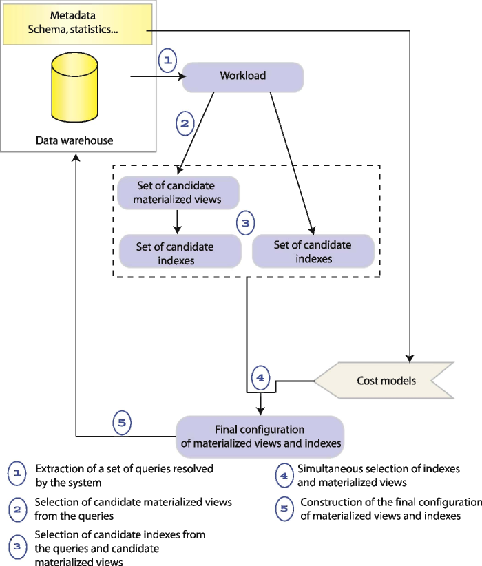
Figure 4: Joint materialized view and index selection approach

4.3.2 Specific data structures

After building the set of candidate materialized views, indexes and indexes on views $O_{C}$, we aim at combining them to recommend a pertinent configuration of materialized views and indexes $O$. To consider the relationships between these objects in this process, we need to materialize them. For this purpose, we use three binary matrices: the “query-view” matrix, the “query-index” matrix and the “view-index” matrix that we detail in the following paragraphs.

To better illustrate how these data structures are designed, let us consider the workload sample from Figure 5. Candidate materialized views and indexes obtained from this workload by applying our strategy are featured in Figures 6 and 7, respectively.

$q_{1}$	select sales.time_id, sum(amount_sold)	$q_{5}$	select promotions.promo_name,
	from sales, times		sum(amount_sold)
	where sales.time_id = times.time_id		from sales, promotions
	and times.time_fiscal_year = 2000		where sales.promo_id = promotions.promo_id
	group by sales.time_id		and promotions.promo_begin_date=‘30/01/2000’
			and promotions.promo_end_date=‘30/03/2000’
			group by promotions.promo_name
$q_{2}$	select sales.prod_id,	$q_{6}$	select customers.cust_marital_status,
	sum(amount_sold)		sum(quantity_sold)
	from sales, products, promotions		from sales, customers, products
	where sales.prod_id = products.prod_id		where sales.cust_id = customers.cust_id
	and sales.promo_id = promotions.promo_id		and sales.prod_id = products.prod_id
	and promotions.promo_category = ‘news paper’		and customers.cust_gender = ‘woman’
	group by sales.prod_id		and products.prod_name = ‘shampooing’
			group by customers.cust_first_name
$q_{3}$	select customers.cust_gender, sum(amount_sold)	$q_{7}$	select products.prod_name, sum(amount_sold)
	from sales, customers, products,		from sales, products, promotions
	where sales.cust_id = customers.cust_id		where sales.prod_id = products. prod_id
	and sales.prod_id = products.prod_id		and sales.promo_id =promotions.promo_id
	and customers.cust_marital_status =‘single’		and products.prod_category=‘tee shirt’
	and products.prod_category = ‘women’		and promotions.promo_end_date=‘30/04/2000’
	group by customers.cust_gender		group by products.prod_name
$q_{4}$	select products.prod_name, sum(amount_sold)	$q_{8}$	select channels.channel_desc, sum(quantity_sold)
	from sales, products, promotions		from sales, channels
	where sales.prod_id = products.prod_id		where sales.channel_id = channels.channel_id
	and sales.promo_id = promotions.prom_id		and channels.channel_class = ‘Internet’
	and promotions.promo_category = ‘TV’		group by channels.channel_desc
	group by products.prod_name

Figure 5: Sample workload

$v_{1}$	create materialized view $v_{1}$ as
	select sales.time_id, times.time_fiscal_year,
	sum(amount_sold)
	from sales, times
	where sales.time_id = times.time_id
	group by sales.time_id, times.times_fiscal_year
$v_{2}$	create materialized view $v_{2}$ as
	select sales.prod_id, sales.cust_id, channels.channel_desc,
	channels.channel_class, sum(quantity_sold)
	from sales, channels, products, customers
	where sales.prod_id = products.prod_id
	and sales.channel_id = channels.channel_id
	and sales.cust_id = customers.cust_id
	group by sales.prod_id, sales.cust_id, channels.channel_desc,
	channels.channel_class
$v_{3}$	create materialized view $v_{3}$ as
	select customers.cust_first_name, products.prod_name,
	products.prod_category, customers.cust_gender,
	customers.cust_marital_status, sum(sales.quantity_sold)
	from sales, customers, products
	where sales.cust_id = customers.cust_id
	and sales.prod_id = products.prod_id
	group by customers.cust_first_name, products.prod_name,
	products.prod_category, customers.cust_gender,
	customers.cust_marital_status
$v_{4}$	create materialized view $v_{4}$ as
	select products.prod_name, products.prod_category,
	promotions.promo_category, sum(amount_sold)
	from sales, products, promotions
	where sales.prod_id = products.prod_id
	and sales.promo_id = promotions.promo_id
	group by products.prod_name, products.prod_category,
	promotions.promo_category
$v_{5}$	create materialized view $v_{5}$ as
	select sales.prod_id, products.prod_category,
	promotions.promo_category, sum(amount_sold)
	from sales, products, promotions
	where sales.prod_id = = products.prod_id
	and sales.promo_id = promotions.promo_id
$v_{6}$	create materialized view $v_{6}$ as
	select channels.channel_class, products.prod_name, channels.channel_desc,
	products.prod_category, sum(sales.quantity_sold), sum(sales.amount_sold)
	from sales, channels, products
	where sales.prod_id = products.prod_id
	and sales.channel_id = channels.channel_id
	group by channels.channel_class, products.prod_name,
	products.prod_category, channels.channel_desc
$v_{7}$	create materialized view $v_{7}$ as
	select sales.prod_id, products.prod_category,
	channels.channel_desc, promotions.promo_name,
	promotions.promo_begin_date, promotions.promo_end_date,
	products.prod_name, sum(sales.quantity_sold), sum(sales.amount_sold)
	from sales, products, promotions
	where sales.prod_id = products.prod_id
	and sales.promo_id = promotions.promo_id
	and sales.channel_id = channels.channel_id
	group by sales.prod_id, products.prod_category, channels.channel_desc,
	promotions.promo_name, promotions.promo_begin_date,
	promotions.promo_end_date, products.prod_name

Figure 6: Candidate materialized views

Indexes	Indexed attributes
$i_{1}$	promotions.promo_category
$i_{2}$	channels.channel_desc
$i_{3}$	channels.channel_class
$i_{4}$	customers.cust_marital_status
$i_{5}$	customers.cust_gender
$i_{6}$	times.time_begin_date
$i_{7}$	times.time_end_date
$i_{8}$	times.fiscal_year
$i_{9}$	products.prod_name
$i_{10}$	products.prod_category
$i_{11}$	promotions.promo_name
$i_{12}$	customers.cust_first_name

Figure 7: Candidate indexes

Query-view matrix.

The query-view matrix ($QV$) captures existing relationships between workload queries and the materialized views extracted from these queries, i.e., views that are exploited by at least one workload query. This matrix may be viewed as the result of rewriting queries with respect to candidate materialized views. The query-view matrix’ rows and columns are workload queries and candidate materialized views, respectively. Its general term $QV_{qv}$ is equal to one if a given query $q$ exploits the corresponding view $v$, and to zero otherwise. Table 2 presents the query-view matrix corresponding to the example from Figures 5 and 6.

	$v_{1}$	$v_{2}$	$v_{3}$	$v_{4}$	$v_{5}$	$v_{6}$	$v_{7}$
$q_{1}$	1	0	0	0	0	0	0
$q_{2}$	0	0	0	1	0	0	0
$q_{3}$	0	0	1	0	0	0	0
$q_{4}$	0	0	0	1	0	0	0
$q_{5}$	0	0	0	0	0	0	1
$q_{6}$	0	0	1	0	0	0	0
$q_{7}$	0	0	0	0	0	0	1
$q_{8}$	0	1	0	0	0	1	0

Table 2: Sample query-view matrix

Query-index matrix.

The query-index matrix ($QI$) stores the indexes built on base tables. This matrix may be viewed as the result of rewriting queries with respect to candidate indexes. The query-index matrix’ rows and columns are workload queries and candidate indexes, respectively. Its general term $QI_{qi}$ is equal to one if a given query $q$ exploits the corresponding index $i$, and to zero otherwise. Table 3 presents the query-index matrix corresponding to the example from Figures 5 and 7.

	$i_{1}$	$i_{2}$	$i_{3}$	$i_{4}$	$i_{5}$	$i_{6}$	$i_{7}$	$i_{8}$	$i_{9}$	$i_{10}$	$i_{11}$	$i_{12}$
$q_{1}$	0	0	0	0	0	0	0	1	0	0	0	0
$q_{2}$	1	0	0	0	0	0	0	0	0	0	0	0
$q_{3}$	0	0	0	1	1	0	0	0	0	1	0	0
$q_{4}$	1	0	0	0	0	0	0	0	1	0	0	0
$q_{5}$	0	0	0	0	1	1	0	0	0	0	1	0
$q_{6}$	0	0	0	0	1	0	0	0	1	0	0	1
$q_{7}$	0	0	0	0	0	0	1	0	1	1	0	0
$q_{8}$	0	1	1	0	0	0	0	0	0	0	0	0

Table 3: Sample query-index matrix

View-index matrix.

The view-index matrix ($VI$) identifies candidate indexes that are recommended for candidate materialized views returned by our view selection algorithm. The query-index matrix’ rows and columns are candidate views and candidate indexes on these views, respectively. Its general term $VI_{vi}$ is equal to one if a given materialized view $v$ exploits the corresponding index $i$, and to zero otherwise. Table 4 presents the view-index matrix corresponding to the example from Figures 6 and 7.

	$i_{1}$	$i_{2}$	$i_{3}$	$i_{4}$	$i_{5}$	$i_{6}$	$i_{7}$	$i_{8}$	$i_{9}$	$i_{10}$	$i_{11}$	$i_{12}$
$v_{1}$	0	0	0	0	0	0	0	1	0	0	0	0
$v_{2}$	0	1	0	0	0	0	0	0	0	0	0	0
$v_{3}$	0	0	0	1	1	0	0	0	1	1	0	1
$v_{4}$	1	0	0	0	0	0	0	0	1	1	0	0
$v_{5}$	1	0	0	0	0	0	0	0	0	1	0	0
$v_{6}$	0	1	1	0	0	0	0	0	1	1	0	0
$v_{7}$	0	1	0	0	0	1	1	0	1	1	1	0

Table 4: Sample view-index matrix

4.3.3 Cost models

We have already presented in Sections 4.1.2 and 4.2.2 cost models relative to materialized views and bitmap join indexes, respectively. Since indexes defined on materialized views are generally B-trees or derivatives, we first recall here the cost models that relate to these indexes. Then, we discuss the benefit of view materialization vs. indexing.

Data access cost through a B-tree index.

Data access through an index is subdivided into to steps: index traversal to find key values corresponding to the query ($C_{traversal}$ cost), and then searching for these identifiers in the database ($C_{search}$ cost). Let $q$ be a query, $\zeta$ a set of indexes, $SNA_{q}$ the set of attributes that are present in query $q$’s restriction clause (the Where clause in SQL), $BF_{a}$ the bloc factor of the index built on attribute $a$ (the average number of $(key,identifier)$ couples per disk page), $SF_{a}$ the selectivity factor of attribute $a$, and finally $v$ the accessed materialized view. Then: $C_{traversal}=\displaystyle{\sum_{a\in(\zeta\cap SNA_{q})}\lceil log_{BF_{a}}|v|\rceil+\left\lceil\frac{SF_{a}|v|}{BF_{a}}\right\rceil-1}$.

The number of identifiers to search for is then $N=|v|\displaystyle{\prod_{a\in(\zeta\cap SNA_{q})}SF_{a}}$. According, to ? (?)’s formula, the number of disk pages to access is: $C_{search}=S_{p}\left(1-(1-\frac{1}{S_{p}})^{N}\right)$, where $S_{p}$ represents disk page size.

Finally, data access cost through a B-tree index is $cost=C_{traversal}+C_{search}$.

B-tree index maintenance cost.

Classically, this cost is expressed as follows:
$maintenance=\displaystyle{\sum_{op\in\{ins,del,upd\}}\displaystyle{\sum f_{op}\displaystyle{\sum_{a\in A_{op}}C_{op}(a)}}}$; where $f_{ins}$, $f_{del}$ and $f_{upd}$ are insert, delete and update frequencies, respectively; and $C_{ins}(a)$, $C_{del}(a)$ and $C_{upd}(a)$ are maintenance costs related to an insert, delete or update operation on attribute $a$, respectively. $A_{op}$ is the set of considered attributes. $A_{ins}=A_{del}=\zeta$, where $\zeta$ is the set of indexes to maintain.
$A_{upd}=\zeta\cap SNA_{upd}$, where $SNA_{upd}$ is the set of attributes to update. Finally, maintenance costs are the following ( ?): $C_{ins}(a)=C_{del}(a)=\lceil log_{BF_{a}}|v|\rceil$ and
$C_{upd}(a)=\lceil log_{BF_{a}}|v|\rceil+\left\lceil\frac{|v|SF_{a}}{2BF_{a}}\right\rceil-1$.

View materialization and indexing benefit.

In the general case (Section 3.4), the benefit brought by selecting an object $o$ is defined as the difference between the execution cost of query workload $Q$ before and after inserting $o$ into the final object configuration $O$. Taking view-index relationships into account implies redefining the benefit function. Let $i\in O_{C}$ and $v\in O_{C}$ be a candidate index and a candidate materialized view, respectively. Adding $i$ or $v$ into $O$ may lead to the benefit cases enumerated in Tables 5 and 6, respectively, depending on interactions between $i$ and $v$.

	$VI_{vi}=1$	$VI_{vi}=0$
$v\in O$	$min$(materialization, indexing $v$)	indexing
$v\not\in O$	—	indexing

Table 5: Benefit brought by index $i$

	$VI_{vi}=1$	$VI_{vi}=0$
$i\in O$	—	materialization
$i\not\in O$	$min$(indexing $v$, materialization)	materialization

Table 6: Benefit brought by materialized view $v$

Indexing and view materialization benefits for $Q$, brought by adding index $i$ or view $v$ into $O$, respectively, may hence be expressed as follows.

$benefit_{O}(i)=\left\{\begin{array}[]{l}\frac{cost(Q,O)-cost(Q,O\cup\{i\})}{size(i)}$~{}if~{}$VI_{vi}=0~{}\forall~{}v\in V~{}(V\subseteq O)\\ \frac{cost(Q,O)-cost(Q,O\cup\{i\}\cup V^{\prime})}{size(i)+\sum{v^{\prime}\in V^{\prime}}size(v^{\prime})}$~{}if~{}$V^{\prime}=\{v\in V,VI_{vi}=1\}\neq\emptyset\\ 0$~{}otherwise$\end{array}\right.$

$benefit_{O}(v)=\left\{\begin{array}[]{l}\frac{cost(Q,O)-cost(Q,O\cup\{v\})}{size(v)}$~{}if~{}$VI_{vi}=0~{}\forall~{}i\in I~{}(I\subseteq O)\\ \frac{cost(Q,O)-cost(Q,O\cup\{v\}\cup I^{\prime})}{size(v)+\sum{i^{\prime}\in I^{\prime}}size(i^{\prime})}$~{}if~{}$I^{\prime}=\{i\in I,VI_{vi}=1\}\neq\emptyset\\ 0$~{}otherwise$\end{array}\right.$

5 Experiments

In order to experimentally validate our generic approach for optimizing data warehouse performance, we have run several series of tests. We summarize the main results in the following sections. Regarding isolate materialized view or index selection, the interested reader can refer to ( ?, ?, ?, ?) for more complete results.

5.1 Experimental conditions

All our tests have been run on a 1 GB data warehouse implemented within Oracle $9i$, on a Pentium 2.4 GHz PC with 512 MB RAM and a 120 GB IDE disk. Our test data warehouse is actually derived from Oracle’s sample data warehouse. Its star schema is composed of one fact table: Sales; and five dimensions: Customers, Products, Times, Promotions and Channels. The workload we executed on this data warehouse is composed of 61 decision-support queries involving aggregation operations and multiple joins between the fact table and dimension tables. Due to space constraints, we do not reproduce here the full data warehouse schema nor the detail of each workload query, but they are both available on-line.

Note that our experiments are based on an ad-hoc benchmark because, at the time we performed them, there was no standard benchmark for data warehouses. TPC-H ( ?) does indeed not feature a true multidimensional schema and thus does not qualify, and TPC-DS’ ( ?) draft specifications had not been issued yet.

5.2 Materialized view selection results

We plotted in Figure 8 the variation of workload execution time with respect to the storage space allotted for materialized views. This figure shows that the views we select significantly improve query execution time. Moreover, execution time decreases when storage space occupation increases. This is predictable because we create more materialized views when storage space $S$ is large and thereby better improve execution time. Let $S_{V}$ be the disk space that is necessary to store all the candidate materialized views. The average gain in performance is indeed 68.9% when $S=35.4\%\times S_{V}$. It is equal to 94.9% when $S=100\%\times S_{V}$ (when the storage space constraint is relaxed).

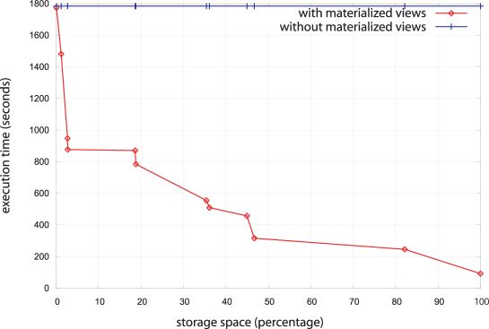
Figure 8: Views materialization experiment results

Moreover, we have demonstrated the relevance of the materialized views that are selected with our approach by computing query cover rate, i.e., the proportion of queries resolved by using views. When the storage space constraint is hard ($S=0.05\%\times S_{V}$), average cover rate is already 23%. It reaches 100% when the storage space constraint is relaxed.

5.3 Index selection results

In these experiments, we have fixed the minimal support parameterized in the Close frequent itemset mining algorithm to 1%. This value gives the highest number of frequent itemsets and consequently the highest number of candidate indexes. This helps vary storage space $S$ within a wide interval. We have measured query execution time according to the percentage of storage space allotted for indexes. This percentage is computed from the space $S_{I}$ occupied by all indexes. Figure 9 shows that execution time decreases when storage space occupation increases. This is predictable because we create more indexes and thus better improve execution time. We also observe that the maximal time gain is about 30% and it is reached for space occupation $S=59.64\%\times S_{I}$.

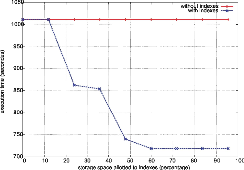
Figure 9: Indexing experiment results

Finally, these experiments also showed that our index selection strategy helped select a portion of candidate indexes that allows to achieve roughly the same performances than the whole set of candidate indexes. This guarantees substantial gains in storage space (40% on an average) and decreases index maintenance cost.

5.4 Joint index and materialized view selection results

Eventually, we have compared the efficiency of isolate materialized view selection, isolate index selection and joint materialized view and index selection. We have measured query execution time in the following cases: without materialized views nor indexes (reference plot), with materialized views only, with indexes only and with both materialized views and indexes (simultaneously selected). Figure 10 represents the variation of response time with respect to the storage space $S$ allotted to materialized views and indexes. $S$ is expressed in percentage of total space $S_{VI}$ occupied by all indexes and materialized views, achieved when we apply our strategy without any storage space constraint. Note that we used a logarithmic scale on the X axis to better visualize the results.

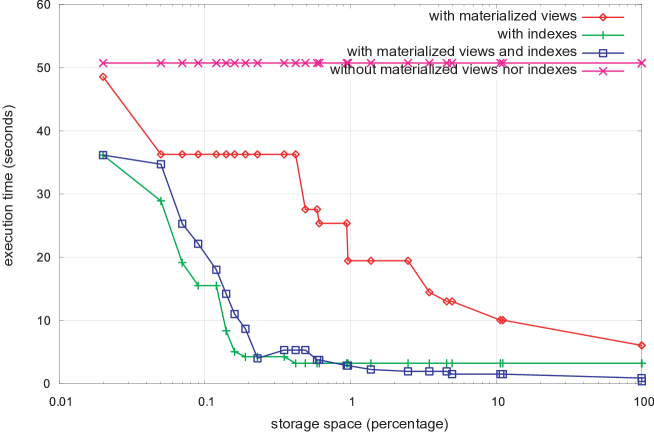
Figure 10: Joint view materialization and indexing experiment results

Figure 10 shows that jointly selecting materialized views and indexes allows better performance than selecting indexes or views separately when storage space is large. However, when it is small, isolate index selection is more competitive than the other solutions. This may be explained by the fact that index size is generally significantly smaller than materialized view size. Then, we can store many more indexes than materialized views in a small space and achieve a better performance. In conclusion, indexes should thus be privileged when storage space is strongly constrained.

6 Conclusion and perspectives

We have presented in this paper an approach for automatic data warehouse performance optimization. Our main contribution in this field mainly relates to exploiting knowledge about the data warehouse and its usage. Knowledge may either be formalized expertise, or automatically extracted with the help of data mining techniques. This approach allowed us to reduce the dimensionality of the materialized view and index selection problem, by proposing a reduced and pertinent candidate object configuration. We also have explicitly taken view-index interactions into account, to propose a final object configuration that is as close as possible to the optimum.

We have designed our approach to be generic. Data mining techniques and cost models we exploit are indeed not related to any system in particular. They may be applied on any host DBMS. Our materialized view and index strategies are also modular: each step (candidate object selection, cost computation…) exploits interchangeable tools. The data mining techniques and cost models we used could easily be replaced by others. Moreover, we could also extend our approach to other performance optimization techniques, such as buffering, physical clustering or partitioning ( ?, ?, ?).

Though we have systematically tried to demonstrate the efficiency of our proposals by experimenting on real-life systems such as Oracle, up to now, we have not been able to compare our proposals to existing approaches in situ. Those that are developed by DMBS vendors ( ?, ?, ?) necessitate the acquisition of the corresponding system. Furthermore, they are implemented as “black boxes” that are often hard to tinker with. Finally, research proposals from the literature are not always available as source or executable code and, when it is the case, they operate in one given environment and must often be reimplemented. We shall have to get over these difficulties to complete our solutions’ experimental validation, though.

Finally, the main possible evolution for our work resides in improving our solutions’ automaticity. We indeed perform static performance optimization. If the input query workload significantly evolves, we must rerun the whole process to preserve performance. Dynamic materialized view selection approaches that have been proposed to optimize refreshing times ( ?, ?) are more efficient than static approaches. We must work in this direction for optimizing query response time.

Our main lead is to exploit our approach’s modularity by replacing the data mining techniques we used by incremental frequent itemset mining ( ?) or clustering ( ?) techniques. Studies related to session detection that are based on entropy computation ( ?) could also be exploited to detect when to rerun the (incremental) selection of materialized views and indexes.

References

- Agrawal and Srikant Agrawal, R., and Srikant, R. (1994). Fast algorithms for mining association rules. In 20th International Conference on Very Large Data Bases, (VLDB 1994), pp. 487–499.
- Agrawal, Chaudhuri, Kollár, Marathe, Narasayya, and Syamala Agrawal, S., Chaudhuri, S., Kollár, L., Marathe, A., Narasayya, V., and Syamala, M. (2004). Database Tuning Advisor for Microsoft SQL Server 2005. In 30th International Conference on Very Large Data Bases (VLDB 2004), Toronto, Canada, pp. 1110–1121.
- Agrawal, Chaudhuri, and Narasayya Agrawal, S., Chaudhuri, S., and Narasayya, V. (2001). Materialized view and index selection tool for Microsoft SQL Server 2000. In ACM SIGMOD International Conference on Management of Data (SIGMOD 2001), Santa Barbara, USA, p. 608.
- Agrawal, Chaudhuri, and Narasayya Agrawal, S., Chaudhuri, S., and Narasayya, V. R. (2000). Automated selection of materialized views and indexes in SQL databases. In 26th International Conference on Very Large Data Bases VLDB 2000, Cairo, Egypt, pp. 496–505.
- Aouiche, Darmont, Boussaïd, and Bentayeb Aouiche, K., Darmont, J., Boussaïd, O., and Bentayeb, F. (2005). Automatic selection of bitmap join indexes in data warehouses. In 7th International Conference on Data Warehousing and Knowledge Discovery (DaWaK 2005), Copenhagen, Denmark, Vol. 3589 of LNCS, pp. 64–73 Heidelberg, Germany. Springer Verlag.
- Aouiche, Darmont, and Gruenwald Aouiche, K., Darmont, J., and Gruenwald, L. (2003). Frequent itemsets mining for database auto-administration. In 7th International Database Engineering and Application Symposium (IDEAS 2003), Hong Kong, China, pp. 98–103.
- Aouiche, Jouve, and Darmont Aouiche, K., Jouve, P., and Darmont, J. (2006). Clustering-Based Materialized View Selection in Data Warehouses. In 10th East-European Conference on Advances in Databases and Information Systems (ADBIS 2006), Thessaloniki, Greece, Vol. 4152 of LNCS, pp. 81–95.
- Baralis, Paraboschi, and Teniente Baralis, E., Paraboschi, S., and Teniente, E. (1997). Materialized views selection in a multidimensional database. In 23rd International Conference on Very Large Data Bases (VLDB 1997), Athens, Greece, pp. 156–165.
- Baril and Bellahsene Baril, X., and Bellahsene, Z. (2003). Selection of materialized views: a cost-based approach. In 15th International Conference on Advanced Information Systems Engineering (CAiSE 2003), Klagenfurt, Austria, pp. 665–680.
- Bellatreche, Boukhalfa, and Mohania Bellatreche, L., Boukhalfa, K., and Mohania, M. (2005). An evolutionary approach to schema partitioning selection in a data warehouse environmen. In 7th International Conference on Data Warehousing and Knowledge Discovery (DaWaK 2005), Copenhagen, Denmark, Vol. 3589 of LNCS, pp. 115–125 Heidelberg, Germany. Springer Verlag.
- Bellatreche, Karlapalem, and Schneider Bellatreche, L., Karlapalem, K., and Schneider, M. (2000). On efficient storage space distribution among materialized views and indices in data warehousing environments. In 9th International Conference on Information and Knowledge Management (CIKM 2000), McLean, USA, pp. 397–404.
- Bruno and Chaudhuri Bruno, N., and Chaudhuri, S. (2006). Physical Design Refinement: The “Merge-Reduce” Approach. In 10th International Conference on Extending Database Technology (EDBT 2006), Munich, Germany, Vol. 3896 of LNCS, pp. 386–404.
- Cardenas Cardenas, A. F. (1975). Analysis and performance of inverted data base structures. Communication of the ACM, 18(5), 253–263.
- Chan, Li, and Feng Chan, G. K. Y., Li, Q., and Feng, L. (1999). Design and selection of materialized views in a data warehousing environment: a case study. In 2nd ACM international workshop on Data warehousing and OLAP (DOLAP 1999), Kansas City, USA, pp. 42–47.
- Chaudhuri, Datar, and Narasayya Chaudhuri, S., Datar, M., and Narasayya, V. (2004). Index selection for databases: A hardness study and a principled heuristic solution. IEEE Transactions on Knowledge and Data Engineering, 16(11), 1313–1323.
- Chaudhuri, Gupta, and Narasayya Chaudhuri, S., Gupta, A., and Narasayya, V. (2002). Compressing SQL workloads. In 2002 ACM SIGMOD International Conference on Management of Data (SIGMOD 2002), Madison, Wisconsin, pp. 488–499.
- Chaudhuri and Narasayya Chaudhuri, S., and Narasayya, V. (1997). An Efficient Cost-Driven Index Selection Tool for Microsoft SQL Server. In 23rd international Conference on Very Large Data Bases (VLDB 1994), Santiago de Chile, Chile, pp. 146–155.
- Chaudhuri and Motwani Chaudhuri, S., and Motwani, R. (1999). On sampling and relational operators. IEEE Data Engineering Bulletin, 22(4), 41–46.
- Choenni, Blanken, and Chang Choenni, S., Blanken, H. M., and Chang, T. (1993a). Index selection in relational databases. In 5th International Conference on Computing and Information (ICCI 1993), Ontario, Canada, pp. 491–496.
- Choenni, Blanken, and Chang Choenni, S., Blanken, H. M., and Chang, T. (1993b). On the selection of secondary indices in relational databases. Data Knowledge Engineering, 11(3), 207–238.
- Comer Comer, D. (1978). The difficulty of optimum index selection. ACM Transactions on Database Systems, 3(4), 440–445.
- Dageville, Das, Dias, Yagoub, Zaït, and Ziauddin Dageville, B., Das, D., Dias, K., Yagoub, K., Zaït, M., and Ziauddin, M. (2004). Automatic SQL Tuning in Oracle 10g. In 30th International Conference on Very Large Data Bases (VLDB 2004), Toronto, Canada, pp. 1098–1109.
- Feldman and Reouven Feldman, Y. A., and Reouven, J. (2003). A knowledge–based approach for index selection in relational databases. Expert System with Applications, 25(1), 15–37.
- Finkelstein, Schkolnick, and Tiberio Finkelstein, S. J., Schkolnick, M., and Tiberio, P. (1988). Physical database design for relational databases. ACM Transactions on Database Systems, 13(1), 91–128.
- Frank, Omiecinski, and Navathe Frank, M. R., Omiecinski, E., and Navathe, S. B. (1992). Adaptive and Automated Index Selection in RDBMS. In 3rd International Conference on Extending Database Technology, (EDBT 1992), Vienna, Austria, Vol. 580 of LNCS, pp. 277–292.
- Goldstein and Åke Larson Goldstein, J., and Åke Larson, P. (2001). Optimizing queries using materialized views: a practical, scalable solution. In ACM SIGMOD international conference on Management of data (SIGMOD 2001), Santa Barbara, USA, pp. 331–342.
- Golfarelli, Rizzi, and Saltarelli Golfarelli, M., Rizzi, S., and Saltarelli, E. (2002). Index selection for data warehousing. In 4th International Workshop on Design and Management of Data Warehouses (DMDW 2002), Toronto, Canada, pp. 33–42.
- Golfarelli and Rizzi Golfarelli, M., and Rizzi, S. (1998). A methodological framework for data warehouse design. In 1st ACM International Workshop on Data Warehousing and OLAP (DOLAP 1998), New York, USA, pp. 3–9.
- Gundem Gundem, T. I. (1999). Near optimal multiple choice index selection for relational databases. Computers & Mathematics with Applications, 37(2), 111–120.
- Gupta Gupta, H. (1999). Selection and Maintenance of Views in a Data Warehouse. Ph.D. thesis, Stanford University.
- Gupta, Harinarayan, Rajaraman, and Ullman Gupta, H., Harinarayan, V., Rajaraman, A., and Ullman, J. D. (1997). Index selection for OLAP. In 13th International Conference on Data Engineering (ICDE 1997), Birmingham, UK, pp. 208–219.
- Gupta and Mumick Gupta, H., and Mumick, I. S. (2005). Selection of views to materialize in a data warehouse. IEEE Transactions on Knowledge and Data Engineering, 17(1), 24–43.
- Harinarayan, Rajaraman, and Ullman Harinarayan, V., Rajaraman, A., and Ullman, J. D. (1996). Implementing data cubes efficiently. In ACM SIGMOD International Conference on Management of data (SIGMOD 1996), Montreal, Canada, pp. 205–216.
- Ip, Saxton, and Raghavan Ip, M. Y. L., Saxton, L. V., and Raghavan, V. V. (1983). On the selection of an optimal set of indexes. IEEE Transactions on Software Engineering, 9(2), 135–143.
- Jain, Murty, and Flynn Jain, A. K., Murty, M. N., and Flynn, P. J. (1999). Data clustering: a review. ACM Computing Surveys, 31(3), 264–323.
- Jouve and Nicoloyannis Jouve, P., and Nicoloyannis, N. (2003). KEROUAC: an algorithm for clustering categorical data sets with practical advantages. In International Workshop on Data Mining for Actionable Knowledge (DMAK 2003), Seoul, Korea.
- Kotidis and Roussopoulos Kotidis, Y., and Roussopoulos, N. (1999). Dynamat: A dynamic view management system for data warehouses. In ACM SIGMOD International Conference on Management of Data (SIGMOD 1999), Philadelphia, USA, pp. 371–382.
- Kratica, Ljubić, and Tošić Kratica, J., Ljubić, I., and Tošić, D. (2003). A genetic algorithm for the index selection problem. In Applications of Evolutionary Computing, EvoWorkshops 2003: EvoBIO, EvoCOP, EvoIASP, EvoMUSART, EvoROB, EvoSTIM, Vol. 2611 of LNCS, pp. 281–291.
- Kyu-Young Kyu-Young, W. (1987). Index Selection in Relational Databases, pp. 497–500. Foundation of Data Organization. Plenum Publishing.
- Labio, Quass, and Adelberg Labio, W., Quass, D., and Adelberg, B. (1997). Physical database design for data warehouses. In 13th International Conference on Data Engineering (ICDE 1997), Birmingham, UK, pp. 277–288.
- Leung, Khan, and Hoque Leung, C., Khan, Q., and Hoque, T. (2005). CanTree: A Tree Structure for Efficient Incremental Mining of Frequent Patterns. In 5th IEEE International Conference on Data Mining (ICDM 2005), Houston, USA, pp. 274–281.
- Mahboubi, Aouiche, and Darmont Mahboubi, H., Aouiche, K., and Darmont, J. (2006). Materialized View Selection by Query Clustering in XML Data Warehouses. In 4th International Multiconference on Computer Science and Information Technology (CSIT 2006), Amman, Jordan, Vol. 2, pp. 68–77.
- Nadeau and Teorey Nadeau, T. P., and Teorey, T. J. (2001). A pareto model for OLAP view size estimation. In 4th Conference of the Centre for Advanced Studies on Collaborative Research (CASCON 2001), Toronto, Canada, p. 13.
- Nadeau and Teorey Nadeau, T. P., and Teorey, T. J. (2002). Achieving scalability in OLAP materialized view selection. In 5th ACM International Workshop on Data Warehousing and OLAP (DOLAP 2002), McLean, USA, pp. 28–34.
- O’Neil and Graefe O’Neil, P., and Graefe, G. (1995). Multi–table joins through bitmapped join indices. SIGMOD Record, 24(3), 8–11.
- O’Neil and Quass O’Neil, P., and Quass, D. (1997). Improved query performance with variant indexes. In ACM SIGMOD International Conference on Management of Data (SIGMOD 1997), Tucson, USA, pp. 38–49.
- Pasquier, Bastide, Taouil, and Lakhal Pasquier, N., Bastide, Y., Taouil, R., and Lakhal, L. (1999). Discovering frequent closed itemsets for association rules. In 7th International Conference on Database Theory (ICDT 1999), Jerusalem, Israel, Vol. 1540 of LNCS, pp. 398–416.
- Rizzi and Saltarelli Rizzi, S., and Saltarelli, E. (2003). View materialization vs. indexing: Balancing space constraints in data warehouse design. In 15th International Conference on Advanced Information Systems Engineering (CAiSE 2003), Klagenfurt, Austria, pp. 502–519.
- Shah, Ramachandran, and Raghavan Shah, B., Ramachandran, K., and Raghavan, V. (2006). A Hybrid Approach for Data Warehouse View Selection. International Journal of Data Warehousing and Mining, 2(2), 1–37.
- Shukla, Deshpande, and Naughton Shukla, A., Deshpande, P., and Naughton, J. F. (2000). Materialized view selection for multi-cube data models. In 7th International Conference on Extending DataBase Technology (EDBT 2000), Konstanz, Germany, pp. 269–284.
- Shukla, Deshpande, Naughton, and Ramasamy Shukla, A., Deshpande, P. M., Naughton, J. F., and Ramasamy, K. (1996). Storage estimation for multidimensional aggregates in the presence of hierarchies. In 22nd International Conference on Very Large Data Bases (VLDB 1996), Bombay, India, pp. 522–531.
- Sismanis, Deligiannakis, Roussopoulos, and Kotidis Sismanis, Y., Deligiannakis, A., Roussopoulos, N., and Kotidis, Y. (2002). Dwarf: shrinking the petacube. In ACM SIGMOD International Conference on Management of Data (SIGMOD 2002), Madison, USA, pp. 464–475.
- Smith, Li, and Jhingran Smith, J. R., Li, C.-S., and Jhingran, A. (2004). A wavelet framework for adapting data cube views for OLAP. IEEE Transactions on Knowledge and Data Engineering, 16(5), 552–565.
- TPC TPC (2005). TPC Benchmark H Standard Specification revision 2.3.0. Transaction Processing Performance Council.
- TPC TPC (2007). TPC Benchmark DS Standard Specification, Draft Version 52. Transaction Processing Performance Council.
- Uchiyama, Runapongsa, and Teorey Uchiyama, H., Runapongsa, K., and Teorey, T. J. (1999). A progressive view materialization algorithm. In 2nd ACM International Workshop on Data warehousing and OLAP (DOLAP 1999), Kansas City, USA, pp. 36–41.
- Valentin, Zuliani, Zilio, Lohman, and Skelley Valentin, G., Zuliani, M., Zilio, D., Lohman, G., and Skelley, A. (2000). DB2 advisor: An optimizer smart enough to recommend its own indexes. In 16th International Conference on Data Engineering, (ICDE 2000), California, USA, pp. 101–110.
- Valluri, Vadapalli, and Karlapalem Valluri, S. R., Vadapalli, S., and Karlapalem, K. (2002). View relevance driven materialized view selection in data warehousing environment. In 13th Australasian Database Technologies (ADC 2002), Melbourne, Australia, pp. 187–196.
- Whang Whang, K. (1985). Index selection in relational databases. In International Conference on Foundations of Data Organization (FODO 1985), Kyoto, Japan, pp. 487–500.
- Wu and Buchmann Wu, M., and Buchmann, A. (1998). Encoded bitmap indexing for data warehouses. In 14th International Conference on Data Engineering (ICDE 1998), Orlando, USA, pp. 220–230.
- Yao, Huang, and An Yao, Q., Huang, J., and An, A. (2005). Machine learning approach to identify database sessions using unlabeled data. In 7th International Conference on Data Warehousing and Knowledge Discovery (DaWaK 2005), Copenhagen, Denmark, Vol. 3589 of LNCS, pp. 254–255.
- Yao Yao, S. B. (1977). Approximating block accesses in database organizations. Communications of the ACM, 20(4), 260–261.
- Zaman, Surabattula, and Gruenwald Zaman, M., Surabattula, J., and Gruenwald, L. (2004). An Auto-Indexing Technique for Databases Based on Clustering. In 15th International Workshop on Database and Expert Systems Applications (DEXA Workshops 2004), Zaragoza, Spain, pp. 776–780.
- Zilio, Rao, Lightstone, Lohman, Storm, Garcia-Arellano, and Fadden Zilio, D., Rao, J., Lightstone, S., Lohman, G., Storm, A., Garcia-Arellano, C., and Fadden, S. (2004). DB2 Design Advisor: Integrated Automatic Physical Database Design. In 30th International Conference on Very Large Data Bases (VLDB 2004), Toronto, Canada, pp. 1087–1097.