Secant dimensions of low-dimensional homogeneous varieties

Abstract.

We completely describe the higher secant dimensions of all connected homogeneous projective varieties of dimension at most $3$, in all possible equivariant embeddings. In particular, we calculate these dimensions for all Segre-Veronese embeddings of ${\mathbb{P}}^{1}\times{\mathbb{P}}^{1}$, ${\mathbb{P}}^{1}\times{\mathbb{P}}^{1}\times{\mathbb{P}}^{1}$, and ${\mathbb{P}}^{2}\times{\mathbb{P}}^{1}$, as well as for the variety $\mathcal{F}$ of incident point-line pairs in ${\mathbb{P}}^{2}$. For ${\mathbb{P}}^{2}\times{\mathbb{P}}^{1}$ and $\mathcal{F}$ the results are new, while the proofs for the other two varieties are more compact than existing proofs. Our main tool is the second author’s tropical approach to secant dimensions.

1. Introduction and results

Let $K$ be an algebraically closed field of characteristic $0$; all varieties appearing here will be over $K$. Let $G$ be a connected affine algebraic group, and let $X$ be a projective variety on which $G$ acts transitively. An equivariant embedding of $X$ is by definition a $G$-equivariant injective morphism $\iota:X\rightarrow{\mathbb{P}}(V)$, where $V$ is a finite-dimensional (rational) $G$-module, subject to the additional constraint that $\iota(X)$ spans ${\mathbb{P}}(V)$. The $k$-th (higher) secant variety $k\iota(X)$ of $\iota(X)$ is the closure in ${\mathbb{P}}(V)$ of the union of all subspaces of ${\mathbb{P}}(V)$ spanned by $k$ points on $\iota(X)$. The expected dimension of $k\iota(X)$ is $\min\{k(\dim X+1)-1,\dim V-1\}$; this is always an upper bound on $\dim k\iota(X)$. We call $k\iota(X)$ non-defective if it has the expected dimension, and defective otherwise. We call $\iota$ non-defective if $k\iota(X)$ is non-defective for all $k$, and defective otherwise.

We want to compute the secant dimensions of $\iota(X)$ for all $X$ of dimension at most $3$ and all $\iota$. This statement really concerns only finitely many pairs $(G,X)$: Indeed, as $X$ is projective and $G$-homogeneous, the stabiliser of any point in $X$ is parabolic (see [2, §11]) and therefore contains the solvable radical $R$ of $G$. But then $R$ also acts trivially on the span of $\iota(X)$, which is ${\mathbb{P}}(V)$, so that we may replace $G$ by the quotient $G/R$, which is semisimple. In addition, we may and will assume that $G$ is simply connected. Now $V$ is an irreducible $G$-module, and $\iota(X)$ is the unique closed orbit of $G$ in ${\mathbb{P}}V$, the cone over which in $V$ is also known as the cone of highest weight vectors. Conversely, recall that for two dominant weights $\lambda$ and $\lambda^{\prime}$ the minimal orbits in the corresponding projective spaces ${\mathbb{P}}V(\lambda)$ and ${\mathbb{P}}V(\lambda^{\prime})$ are isomorphic (as $G$-varieties) if and only if $\lambda$ and $\lambda^{\prime}$ have the same support on the basis of fundamental weights. So, to prove that all equivariant embeddings of a fixed $X$ are non-degenerate, we have to consider all possible dominant weights with a fixed support.

Now there are precisely seven pairs $(G,X)$ with $\dim X\leq 3$, namely $(\mathrm{SL}_{2}^{i},({\mathbb{P}}^{1})^{i})$ for $i=1,2,3$, $(\mathrm{SL}_{3},{\mathbb{P}}^{2})$, $(\mathrm{SL}_{3}\times\mathrm{SL}_{2},{\mathbb{P}}^{2}\times{\mathbb{P}}^{1})$, $(\mathrm{SL}_{4},{\mathbb{P}}^{3})$, and $(\mathrm{SL}_{3},\mathcal{F})$, where $\mathcal{F}$ is the variety of flags $p\subset l$ with $p,l$ a point and a line in ${\mathbb{P}}^{2}$, respectively. The equivariant embeddings of ${\mathbb{P}}^{i}$ for $i=1,2,3$ are the Veronese embeddings; their higher secant dimensions—and indeed, all higher secant dimensions of Veronese embeddings of projective spaces of arbitrary dimensions—are known from the work of Alexander and Hirschowitz [1]. In low dimensions there also exist tropical proofs for these results: ${\mathbb{P}}^{1}$ and ${\mathbb{P}}^{2}$ were given as examples in [8], and for ${\mathbb{P}}^{3}$ see the Master’s thesis of Silvia Brannetti [3]. The other varieties are covered by the following theorems.

First, the equivariant embeddings of ${\mathbb{P}}^{1}\times{\mathbb{P}}^{1}$ are the Segre-Veronese embeddings, parametrised by the degree $(d,e)$ (corresponding to the highest weight $d\omega_{1}+e\omega_{2}$ where the $\omega_{i}$ are the fundamental weights), where we may assume $d\geq e$. The following theorem is known in the literature; see for instance [4, Theorem 2.1] and the references there. Our proof is rather short and transparent, and serves as a good introduction to the more complicated proofs of the remaining theorems.

Theorem 1.1.

The Segre-Veronese embedding of ${\mathbb{P}}^{1}\times{\mathbb{P}}^{1}$ of degree $(d,e)$ with $d\geq e\geq 1$ is non-defective unless $e=2$ and $d$ is even, in which case the $(d+1)$-st secant variety has codimension $1$ rather than the expected $0$.

The equivariant embeddings of ${\mathbb{P}}^{1}\times{\mathbb{P}}^{1}\times{\mathbb{P}}^{1}$ and of ${\mathbb{P}}^{2}\times{\mathbb{P}}^{1}$ are also Segre-Veronese embeddings. While writing this paper we found out that the following theorem has already been proved in [5]. We include our proof because we need its building blocks for the other $3$-dimensional varieties.

Theorem 1.2.

The Segre-Veronese embedding of ${\mathbb{P}}^{1}\times{\mathbb{P}}^{1}\times{\mathbb{P}}^{1}$ of degree $(d,e,f)$ with $d\geq e\geq f\geq 1$ is non-defective unless

1. $e=f=1$ and $d$ is even, in which case the $(d+1)$-st secant variety has codimension $1$ rather than the expected $0$, or

2. $d=e=f=2$, in which case the $7$-th secant variety has codimension $1$ instead of the expected $0$.

Theorem 1.3.

The Segre-Veronese embedding of ${\mathbb{P}}^{2}\times{\mathbb{P}}^{1}$ of degree $(d,e)$ with $d,e\geq 1$ is non-defective unless

1. $d=2$ and $e=2k$ is even, in which case the $(3k+1)$-st secant variety has codimension $3$ rather than the expected $2$ and the $(3k+2)$-nd secant variety has codimension $1$ rather than $0$; or

2. $d=3$ and $e=1$, in which case the $5$-th secant variety has codimension $1$ rather than the expected $0$.

Finally, the equivariant embeddings of $\mathcal{F}$ are the minimal orbits in ${\mathbb{P}}V$ for any irreducible $\mathrm{SL}_{3}$-representation of highest weight $d\omega_{1}+e\omega_{2}$.

Theorem 1.4.

The image of $\mathcal{F}$ in ${\mathbb{P}}V$, for $V$ an irreducible $\mathrm{SL}_{3}$-representation of highest weight $d\omega_{1}+e\omega_{2}$ with $d,e\geq 1$ is non-defective unless

1. $d=e=1$, in which the $2$nd secant variety has codimension $1$ rather than $0$, or

2. $d=e=2$, in which the $7$th secant variety has codimension $1$ rather than $0$.

To the best of our knowledge Theorems 1.3 and 1.4 are new. Moreover, $\mathcal{F}$ seems to be the first settled case where maximal tori in $G$ do not have dense orbits. Our proofs of Theorems 1.1 and 1.2 are more compact than their original proofs [4, 5]. Moreover, the planar proof of Theorem 1.1 serves as a good introduction to the more complicated induction in the three-dimensional cases, while parts of the proof of Theorem 1.2 are used as building blocks in the remaining proofs.

We will prove our theorems using a polyhedral-combinatorial lower bound on higher secant dimensions introduced by the second author in [8]. Roughly this goes as follows: to a given $X$ and $V$ we associate a finite set $B$ of points in ${\mathbb{R}}^{\dim X}$, which parametrises a certain basis in $V$. Now to find a lower bound on $\dim kX$ we maximise

$$\sum_{i=1}^{k}[1+\dim\operatorname{Aff}\nolimits_{\mathbb{R}}\operatorname{Win}_{i}(f)]$$

over all $k$-tuples $f=(f_{1},\ldots,f_{n})$ of affine-linear functions on ${\mathbb{R}}^{\dim X}$, where $\operatorname{Win}_{i}(f)$ is the set of points in $B$ where $f_{i}$ is strictly smaller than all $f_{j}$ with $j\neq i$, and where $\operatorname{Aff}\nolimits_{\mathbb{R}}$ denotes taking the affine span. Typically, this maximum equals $1$ plus the expected dimension of $\dim k\iota(X)$, and then we are done. If not, then we need other methods to prove that $k\iota(X)$ is indeed defective—but most defective cases above are known in the literature.

This optimisation problem may sound somewhat far-fetched, so as a motivation we now carry out our proof in one particular case: For the Segre-Veronese embedding of $X={\mathbb{P}}^{1}\times{\mathbb{P}}^{1}$ of degree $(d,e)$ the set $B$ is the grid $\{0,\ldots,d\}\times\{0,\ldots,e\}\subseteq{\mathbb{R}}^{2}$. Take for instance $d=3$ and $e=2$. In Figure 1 the points in $B$ are grouped into four triples spanning the plane. It is easy to see—see Lemma 2.4 below—that there exist affine-linear $f_{1},\ldots,f_{4}$ inducing this partition, so that $4X$ has the expected dimension $4\cdot 3-1=11$.

Figure 1. The embedding $\operatorname{Seg}\nolimits\circ(v_{3}\times v_{2})$ of ${\mathbb{P}}^{1}\times{\mathbb{P}}^{1}$ is non-defective.

Our tropical approach is conceptually very simple, and closely related to Sturmfels-Sullivant’s combinatorial secant varieties [10], Miranda-Dumitrescu’s degeneration approach (private communication), and Develin’s tropical secant varieties of linear spaces [7]. What we find very surprising and promising is that strong results on secant varieties of non-toric varieties such as $\mathcal{F}$ can be proved with our approach.

The remainder of this paper is organised as follows. In Section 2 we recall the tropical approach, and prove a lemma that will help us deal with the flag variety. The tropical approach depends rather heavily on a parameterisation of $X$, and in Section 3 we introduce the polynomial maps that we will use. In particular, we give, for any minimal orbit (not necessarily of low dimension, and not necessarily toric), a polynomial paramaterisation whose tropicalisation has an image of the right dimension; these tropical parameterisations are useful in studying tropicalisations of minimal orbits; see Remark 3.3. Finally, Sections 4–7 contain the proofs of Theorems 1.1–1.4, respectively.

2. The tropical approach

2.1. Two optimisation problems

We recall from [8] a polyhedral-combinatorial optimisation problem that plays a crucial role in the proofs of our theorems; here $\operatorname{AP}$ abbreviates Affine Partition.

Problem 2.1 ($\operatorname{AP}(A,k)$).

Let $A=(A_{1},\ldots,A_{n})$ be a sequence of finite subsets of ${\mathbb{R}}^{m}$ and let $k\in{\mathbb{N}}$. For any $k$-tuple $f=(f_{1},\ldots,f_{k})$ of affine-linear functions on ${\mathbb{R}}^{m}$ let the sets $\operatorname{Win}\nolimits_{i}(f),\ i=1,\ldots,k$ be defined as follows. For $b=1,\ldots,n$ we say that $f_{i}$ wins $b$ if $f_{i}$ attains its minimum on $A_{b}$ in a unique $\alpha\in A_{b}$, and if this minimum is strictly smaller than all values of all $f_{j},j\neq i$ on $A_{b}$. The vector $\alpha$ is then called a winning direction of $f_{i}$. Let $\operatorname{Win}\nolimits_{i}(f)$ denote the set of winning directions of $f_{i}$.

Maximise $\sum_{i=1}^{k}[1+\dim\operatorname{Aff}\nolimits_{\mathbb{R}}\operatorname{Win}\nolimits_{i}(f)]$ over all $k$-tuples $f$ of affine-linear functions on ${\mathbb{R}}^{m}$; call the maximum $\operatorname{AP}^{*}(A,k)$.

Note that if every $A_{b}$ is a singleton $\{\alpha_{b}\}$, then $\operatorname{Win}\nolimits_{i}(f)$ is just the set of all $\alpha_{b}$ on which $f_{i}$ is smaller than all other $f_{j},j\neq i$. We will then also write $\operatorname{AP}(\{\alpha_{1},\ldots,\alpha_{n}\},k)$ for the optimisation problem above. In this case we are really optimising over all possible regular subdivisions of ${\mathbb{R}}^{m}$ into $k$ open cells. Each such subdivision induces a partition of the $\alpha_{b}$ into the sets $\operatorname{Win}\nolimits_{i}(f)$ (at least if no $\alpha_{b}$ lies on a border between two cells, but this is easy to achieve without decreasing the objective function). As it is sometimes hard to imagine the existence of affine-linear functions inducing a certain regular subdivision of space, we have the following observation, due to Immanuel Halupczok and the second author.

Lemma 2.2.

Let $S$ be a finite set in ${\mathbb{R}}^{m}$, let $f_{1},\ldots,f_{k}$ be affine-linear functions on ${\mathbb{R}}^{m}$, and let $g_{1},\ldots,g_{l}$ also be affine-linear functions on ${\mathbb{R}}^{m}$. Let $S_{i}$ be the subset of $S$ where $f_{i}<f_{j}$ for all $j\neq i$, and let $T_{i}$ be the subset of $S_{1}$ where $g_{i}<g_{j}$ for all $j\neq i$. Then there exist affine-linear functions $h_{1},\ldots,h_{l}$ such that

1. $h_{i}<h_{j}$ on $T_{i}$ for $i,j=1,\ldots,l$ and $j\neq i$;

2. $h_{i}<f_{j}$ on $T_{i}$ for $i=1,\ldots,l$ and $j=2,\ldots,k$; and

3. $f_{i}<h_{j}$ on $S_{i}$ for $i=2,\ldots,k$ and $j=1,\ldots,l$.

In other words, the functions $h_{1},\ldots,h_{l},f_{2},\ldots,f_{k}$ together induce the partition $T_{1},\ldots,T_{l},S_{2},\ldots,S_{k}$ of $S$.

Proof.

Take $h_{i}=f_{1}+\epsilon g_{i}$ for $\epsilon$ positive and sufficiently small. ∎

This lemma implies, for instance, that one may find appropriate $\operatorname{Win}\nolimits_{i}(f)$ (still for the case of singletons $A_{b}$) by repeatedly cutting polyhedral pieces of space in half. For instance, in Figure 1 the plane is cut into four pieces by three straight cuts. Although this is not a regular subdivision of the plane, by the lemma there does exist a regular subdivision of the plane inducing the same partition on the $12$ points.

Lemma 2.2 can only immediately be applied to $\operatorname{AP}$ if the $A_{b}$ are singletons, while the $A_{b}$ in our application to the $3$-dimensional flag variety $\mathcal{F}$ are not. We get around this difficulty by giving a lower bound on $\operatorname{AP}^{*}(A,k)$ for more general $A$ in terms of $\operatorname{AP}^{*}(A^{\prime},k)$ for some sequence $A^{\prime}$ of singletons. In the following lemmas a convex polyhedral cone in ${\mathbb{R}}^{m}$ is by definition the set of nonnegative linear combinations of a finite set in ${\mathbb{R}}^{m}$, and it is called strictly convex if it does not contain any non-trivial linear subspace of ${\mathbb{R}}^{m}$.

Lemma 2.3.

Let $A=(\{\alpha_{1}\},\ldots,\{\alpha_{n}\})$ be an $n$-tuple of singleton subsets of ${\mathbb{R}}^{m}$. Furthermore, let $k\in{\mathbb{N}}$, let $Z$ be a strictly convex polyhedral cone in ${\mathbb{R}}^{m}$, and let $f$ be a $k$-tuple of affine-linear functions on ${\mathbb{R}}^{m}$. Then the value of $\operatorname{AP}(A,k)$ at $f$ is also attained at some $f^{\prime}=(f_{1}^{\prime},\ldots,f_{k}^{\prime})$ for which every $f_{i}^{\prime}$ is strictly decreasing in the $z$-direction, for every $z\in Z\setminus\{0\}$.

Proof.

By the strict convexity of $Z$, there exists a linear function $f_{0}$ on ${\mathbb{R}}^{m}$ such that every $f_{j}+f_{0}$ is strictly decreasing in the $z$-direction, for every $z\in Z$. But since

$$f_{i}(\alpha)<f_{j}(\alpha)\Leftrightarrow f_{i}(\alpha)+f_{0}(\alpha)<f_{j}(\alpha)+f_{0}(\alpha)$$

we have $\operatorname{Win}\nolimits_{i}((f_{j}+f_{0})_{j})=\operatorname{Win}\nolimits_{i}(f)$ for all $i$, and we are done. ∎

It is crucial in this proof that only values of $f_{i}$ and $f_{j}$ at the same $\alpha$ are compared—that is why we have restricted ourselves to singleton-$\operatorname{AP}$ here.

Lemma 2.4.

Let $A=(A_{1},\ldots,A_{n})$ be a $k$-tuple of finite subsets of ${\mathbb{R}}^{m}$ and let $k\in{\mathbb{N}}$. Furthermore, let $Z$ be a strictly convex polyhedral cone in ${\mathbb{R}}^{m}$ and define a partial order $\leq$ on ${\mathbb{R}}^{m}$ by

$$p\leq q:\Leftrightarrow p-q\in Z.$$

Suppose that for every $b$, $A_{b}$ has a unique minimal element $\alpha_{b}$ with respect to this order. Then we have

$$\operatorname{AP}^{*}(A,k)\geq\operatorname{AP}^{*}(\{\alpha_{1},\ldots,\alpha_{n}\},k)$$

Proof.

Let $d^{*}=\operatorname{AP}^{*}(\{\alpha_{1},\ldots,\alpha_{n}\},k)$. By Lemma 2.3 there exists a $k$-tuple $f=(f_{1},\ldots,f_{k})$ of affine-linear functions on ${\mathbb{R}}^{m}$ for which $\operatorname{AP}(\{\alpha_{1},\ldots,\alpha_{n}\},k)$ also has value $d^{*}$ and for which every $f_{i}$ is strictly decreasing in all directions in $Z$. We claim that the value of $\operatorname{AP}(A,k)$ at this $f$ is also $d^{*}$. Indeed, fix $b\in B$ and consider all $f_{i}(\alpha)$ with $\alpha\in A_{b}$ and $i=1,\ldots,k$. Because $\alpha_{b}-\alpha\in Z$ for all $\alpha\in A_{b}$ and because every $f_{i}$ is strictly decreasing in the directions in $Z$, we have $f_{i}(\alpha_{b})<f_{i}(\alpha)$ for all $\alpha\in A_{b}\setminus\{\alpha_{b}\}$ and all $i$. Hence the minimum, over all pairs $(i,\alpha)\in\{1,\ldots,k\}\times A_{b}$, of $f_{i}(\alpha)$ can only be attained in pairs for which $\alpha=\alpha_{b}$. Therefore, in computing the value at $f$ of $\operatorname{AP}(A,k)$ the elements of $A_{b}$ unequal to $\alpha_{b}$ can be ignored. We conclude that $\operatorname{AP}(A,k)$ has value $d^{*}$ at $f$, as claimed. This shows the inequality. ∎

2.2. Tropical bounds on secant dimensions

Rather than working with projective varieties, we work with the affine cones over them. So suppose that $C\subseteq K^{n}$ is a closed cone (i.e., closed under scalar multiplication with $K$), and set

$$kC:=\overline{\{v_{1}+\ldots+v_{k}\mid v_{1},\ldots,v_{k}\in C\}}.$$

Suppose that $C$ is unirational, and choose a polynomial map $f=(f_{1},\ldots,f_{n}):K^{m}\rightarrow C\subseteq K^{n}$ that maps $K^{m}$ dominantly into $C$. Let $x=(x_{i})_{i=1}^{m}$ and $y=(y_{b})_{b=1}^{n}$ be the standard coordinates on $K^{m}$ and $K^{n}$. The tropical approach depends very much on coordinates; in particular, one would like $f$ to be sparse. For every $b=1,\ldots,n$ let $A_{b}$ be the set of $\alpha\in{\mathbb{N}}^{m}$ for which the monomial $x^{\alpha}$ has a non-zero coefficient in $f_{b}$, and set $A:=(A_{1},\ldots,A_{n})$.

Theorem 2.5 ([8]).

For all $k\in{\mathbb{N}}$, $\dim kC\geq\operatorname{AP}^{*}(A,k)$.

Remark 2.6.

In fact, in [8] this is proved provided that $\bigcup_{b}A_{b}$ is contained in an affine hyperplane not through $0$, but this can always be achieved by taking a new map $f^{\prime}(t,x):=tf(x)$ into $C$, without changing the optimisation problem $\operatorname{AP}(A,k)$.

In Section 3 we introduce a polynomial map $f$ for general minimal orbits that seems suitable for the tropical approach, and after that we specialise to low-dimensional varieties under consideration.

2.3. Non-defective pictures

Our proofs will be entirely pictorial: given a set $B$ of lattice points in ${\mathbb{Z}}^{2}$ or ${\mathbb{Z}}^{3}$ according as $\dim X=2$ or $\dim X=3$, we solve the optimisation problem $\operatorname{AP}(B,k)$ for all $k$. To this end, we will exhibit a partition of $B$ into parts $B_{i}$ such that there exist affine-linear functions $f_{i}$ on ${\mathbb{R}}^{2}$ or ${\mathbb{R}}^{3}$, exactly one for each part, with $B_{i}=\operatorname{Win}\nolimits_{i}(f)$. If each $B_{i}$ is affinely independent, and if moreover the affine span of each $B_{i}$ has $\dim X$, except possibly for one single $B_{i}$, then we call the picture non-defective, as it shows, by Theorem 2.5, that all secant varieties of $X$ in the given embedding have the expected dimension.

The full-dimensional $B_{i}$ that we will use will have very simple shapes: in dimension $2$ they will all be equivalent, up to integral translations and rotations over multiples of $\pi/2$, to the triple $\{0,e_{1},e_{2}\}$. In dimension $3$ they will almost all be equivalent to either $\{0,e_{1},e_{2},e_{3}\}$ (type $1$) or $\{e_{1},0,e_{2},e_{2}+e_{3}\}$ (type $2$), up to Euclidean transformations preserving the lattice; see Figure 2. Only in case of the flag-variety $\mathcal{F}$ we will occasionally use more general pictures.

The $f_{i}$ will not be explicitly computed. Indeed, in all cases their existence follows from a tedious but easy application of Lemma 2.2: one can repeatedly cut ${\mathbb{R}}^{2}$ or ${\mathbb{R}}^{3}$ into pieces by affine hyperplanes, such that eventually the desired partition of $B$ into the $B_{i}$ is attained. For instance, in Figure 1 three cuts, labelled $1,2,3$ consecutively, give the desired partition of the twelve points.

Figure 2. Types $1$ (left) and $2$ (right).

3. A polynomial map

We retain the setting of the Introduction: $G$ is a simply connected, connected, semisimple algebraic group, $V$ is a $G$-module, and we wish to determine the secant dimensions of $X$, the unique closed orbit of $G$ in ${\mathbb{P}}V$. Let $C$ be the affine cone in $V$ over $X$. Fix a Borel subgroup $B$ of $G$, let $T$ be a maximal torus of $B$ and let $v_{\lambda}\in V$ span the unique $B$-stable one-dimensional subspace of $V$; $\lambda$ denotes the $T$-weight of $v_{\lambda}$, i.e., the highest weight of $V$. Let $P\supseteq B$ be the stabiliser in $G$ of $Kv_{\lambda}$ (so that $X\cong G/P$ as a $G$-variety) and let $U$ be the unipotent radical of the parabolic subgroup opposite to $P$ and containing $T$. Let $\mathfrak{u}$ denote the Lie algebra of $U_{-}$, let ${X(\mathfrak{u})}$ be the set of $T$-roots on $\mathfrak{u}$, and set $\tilde{X}(\mathfrak{u}):={X(\mathfrak{u})}\cup\{0\}$. For every $\beta\in{X(\mathfrak{u})}$ choose a vector $X_{\beta}$ spanning the root space $\mathfrak{u}_{\beta}$. Moreover, fix an order on ${X(\mathfrak{u})}$. Then it is well-known that the polynomial map

$$\Psi:K^{\tilde{X}(\mathfrak{u})}\rightarrow V,t\mapsto t_{0}\prod_{\beta\in{X(\mathfrak{u})}}\exp(t_{\beta}X_{\beta})v_{\lambda},$$

where the product is taken in the fixed order, maps dominantly into $C$. This map will play the role of $f$ from Subsection 2.2.

In what follows we will need the following notation: Let $X_{\mathbb{R}}:={\mathbb{R}}\otimes_{\mathbb{Z}}X(T)$ be the real vector space spanned by the character group of $T$, let $\xi:{\mathbb{R}}^{{X(\mathfrak{u})}}\mapsto X_{\mathbb{R}}$ send $r$ to $\sum_{\beta}r_{\beta}\beta$ and also use $\xi$ for the map ${\mathbb{R}}^{\tilde{X}(\mathfrak{u})}\rightarrow X_{\mathbb{R}}$ with the same definition; in both cases we call $\xi(r)$ the weight of $r$.

Now for a basis of $V$: by the PBW-theorem, $V$ is the linear span of all elements of the form $m_{r}:=\prod_{\beta\in{X(\mathfrak{u})}}X_{\beta}^{r_{\beta}}v_{\lambda}$ with $r\in{\mathbb{N}}^{{X(\mathfrak{u})}}$; the product is taken in the same fixed order as before. Slightly inaccurately, we will call the $m_{r}$ PBW-monomials. Note that the $T$-weight of $m_{r}$ is $\lambda+\xi(r)$. Let $M$ be the subset of all $r\in{\mathbb{N}}^{{X(\mathfrak{u})}}$ for which $m_{r}$ is non-zero; $M$ is finite. Let $B$ be a subset of $M$ such that $\{m_{r}\mid r\in B\}$ is a basis of $V$; later on we will add further restrictions on $B$. For $b\in B$ let $\Psi_{b}$ be the component of $\Psi$ corresponding to $b$; it equals $t_{0}$ times a polynomial in the $t_{\beta},\ \beta\in{X(\mathfrak{u})}$. Let $A_{b}\subseteq{\mathbb{N}}^{{X(\mathfrak{u})}}$ denote the set of exponent vectors of monomials having a non-zero coefficient in $\Psi_{b}/t_{0}$.

Lemma 3.1.

For $b_{0}\in B$

1. $A_{b_{0}}\subseteq\{r\in M\mid\xi(r)=\xi(b_{0})\}$, and

2. $A_{b_{0}}\cap B=\{b_{0}\}$.

Proof.

Expand $\Psi(t)/t_{0}$ as a linear combination of PBW-monomials:

$$\Psi(t)/t_{0}=\sum_{r\in{\mathbb{N}}^{{X(\mathfrak{u})}}}\frac{t^{r}}{\prod_{\beta\in{X(\mathfrak{u})}}(r_{\beta}!)}m_{r}.$$

So $t^{r}$ appears in $\Psi_{b_{0}}/t_{0}$ if and only if $m_{r}$ has a non-zero $m_{b_{0}}$-coefficient relative to the basis $(m_{b})_{b\in B}$. Hence the first statement follows from the fact that every $m_{r}$ is a linear combination of the $m_{b}$ of the same $T$-weight as $m_{r}$, and the second statement reflects the fact that for all $b_{1}\in B$, $m_{b_{1}}$ has precisely one non-zero coefficient relative to the basis $(m_{b})_{b\in B}$, namely that of $m_{b_{1}}$. ∎

Now Theorem 2.5 implies the following proposition.

Proposition 3.2.

$\dim kC\geq\operatorname{AP}^{*}((A_{b})_{b\in B},k)$

For Segre products of Veronese embeddings every $A_{b}$ is a singleton, and we can use our hyperplane-cutting procedure immediately. For the flag variety $\mathcal{F}$ we will use Lemma 2.4 to bound $\operatorname{AP}^{*}$ by a singleton-$\operatorname{AP}^{*}$.

Remark 3.3.

To see that Proposition 3.2 has a chance of being useful, it is instructive to verify that $\operatorname{AP}^{*}((A_{b})_{b\in B},1)$ is, indeed, $\dim C$, at least for some choices of $B$. Indeed, recall that $|{X(\mathfrak{u})}|+1$ vectors $v_{\lambda}$ and $X_{\beta}v_{\lambda},\beta\in{X(\mathfrak{u})}$ are linearly independent, so that we can take $B$ to contain the corresponding exponent vectors, that is, $0$ and the standard basis vectors $e_{\beta}$ in ${\mathbb{N}}^{X(\mathfrak{u})}$. Now let $f_{1}:{\mathbb{R}}^{{X(\mathfrak{u})}}\rightarrow{\mathbb{R}}$ send $r$ to $\sum_{\beta\in{X(\mathfrak{u})}}r_{\beta}$. We claim that $\operatorname{AP}((A_{b})_{b\in B},k)$ has value $\dim C$ at $(f_{1})$. Indeed, $A_{0}=\{0\}$ and for every $b\in B$ of the form $e_{\beta},\beta\in{X(\mathfrak{u})}$ the set $A_{b}$ consists of $e_{\beta}$ itself, with $f_{1}$-value $1$, and exponent vectors having a $f_{1}$-value a natural number $>1$. Hence $\operatorname{Win}\nolimits_{1}(f_{1})$ contains all $e_{\beta}$ and $0$—and therefore spans an affine space of dimension $\dim C-1=\dim X$.

This observation is of some independent interest for tropical geometry: going through the theory in [8], it shows that the image of the tropicalisation of $\Psi$ in the tropicalisation of $C$ has the right dimension; this is useful in minimal orbits such as Grassmannians.

4. Secant dimensions of ${\mathbb{P}}^{1}\times{\mathbb{P}}^{1}$

We retain the notation of Section 3. To prove Theorem 1.1, let $X={\mathbb{P}}^{1}\times{\mathbb{P}}^{1}$, $G=\mathrm{SL}_{2}\times\mathrm{SL}_{2}$, and $V=S^{d}(K^{2})\otimes S^{e}(K^{2})$. The polynomial map

$$\Psi:(t_{0},t_{1},t_{2})\mapsto t_{0}(x_{1}+t_{1}x_{2})^{d}\otimes(x_{1}+t_{2}x_{2})^{e},$$

is dominant into the cone $C$ over $X$, and $M=B$ is the rectangular grid $\{0,\ldots,d\}\times\{0,\ldots,e\}$. We may assume that $d\geq e$.

First, if $e=2$ and $d$ is even, then $(d+1)C$ is known to be defective, that is, it does not fill $V$ but is given by some determinantal equation; see [9, Example 3.2]. The argument below will show that its defect is not more than $1$.

(a) $(d,e)=(1,1)$

(b) $(d,e)=(2,1)$

(c) $(d,e)=(3,1)$

(d) $e=1$; induction

(e) $(d,e)=(2,2)$

(f) $(d,e)=(3,2)$

(g) $e=2$; induction

(h) $(d,e)=(3,3)$

(i) $(d,e)=(4,3)$

(j) $(d,e)=(5,3)$

(k) $e=3$; induction

(l) $(d,e)=(3,4)$

(m) $(d,e)=(4,4)$

(n) $e=4$, induction

(o) $e=5$; induction

Figure 3 gives non-defective pictures for $e=1,2,3,4,5$ and $d\geq e$, except for $e=2$ and $d$ even. This implies, by transposing pictures, that there exist non-defective pictures for $e=6$ and $d=1,3,4,5$. Figure 3(p) gives a non-defective picture for $(d,e)=(6,6)$. Then, using the two induction steps in Figure 3(q), we find non-defective pictures for $e=6$ and all $d\neq 2$. A similar reasoning gives non-defective pictures for $e=8$ and all $d\neq 2$. Finally, let $d\geq e\geq 6$ be arbitrary with $(d,e)\not\in 2{\mathbb{N}}\times\{2\}$. Write $e+1=6q+r$ with $r\in\{0,2,4,5,7,9\}$. Then we find a non-defective picture for $(d,e)$ by gluing $q$ non-defective pictures for $(d,5)$ and, if $r\neq 0$, one non-defective picture for $(d,r-1)$ on top of each other. This proves Theorem 1.1.

(p) $(d,e)=(6,6)$

(q) $e=6$; induction

(r) $e=8$; induction

Figure 3. More non-defective pictures for ${\mathbb{P}}^{1}\times{\mathbb{P}}^{1}$.

5. Secant dimensions of ${\mathbb{P}}^{1}\times{\mathbb{P}}^{1}\times{\mathbb{P}}^{1}$

Now we turn to Theorem 1.2. Cutting to the chase, $M=B$ is the block $\{0,\ldots,d\}\times\{0,\ldots,e\}\times\{0,\ldots,f\}$. When convenient, we assume that $d\geq e\geq f$. First, for $e=f=1$ and $d$ even, the $d+1$-st secant variety, which one would expect to fill the space, is in fact known to be defective, see [5]. The pictures below will show that the defect is not more than $1$.

(a) $(1,1,1)$

(b) $(2,1,1)$

(c) induction for $(*,1,1)$

(d) $(2,2,1)$

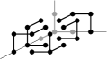
(e) $(3,2,1)$

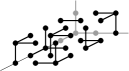
(f) $(4,2,1)$

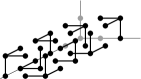
(g) $(5,2,1)$

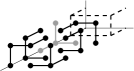
(h) induction for $(*,2,1)$

Figure 4. Non-defective pictures for $(e,f)=(1,1)$ or $(2,1)$

Figure 4 gives inductive constructions for pictures for $(e,f)\in\{(1,1),(2,1)\}$ that are non-defective except for $(e,f)=(1,1)$ and $d$ even. The grey shades serve no other purpose than to distinguish between front and behind.

(a) $(3,3,1)$

(b) induction for $(*,3,1)$

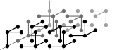
(c) $(4,4,1)$

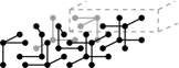
(d) induction for $(*,4,1)$

Figure 5. Non-defective pictures for $(*,3,1)$ and $(*,4,1)$.

Rotating appropriately, this also gives non-defective pictures for $(1,3,1)$ and $(2,3,1)$; Figure 5(b) then gives an inductive construction of non-defective pictures for $(d,3,1)$ for $d\geq 3$.

So far we have found non-defective pictures for $(2,4,1)$ and $(3,4,1)$ (just rotate those for $(4,2,1)$ and $(4,3,1)$). Figure 5(c) gives a non-defective picture for $(4,4,1)$. A non-defective picture for $(5,4,1)$ can be constructed from a non-defective picture for $(5,1,1)$ and one for $(5,2,1)$. Now let $d\geq 6$ and write $d+1=4q+r$ with $q\geq 0$ and $r\in\{3,4,5,6\}$. Then using $q$ copies of our non-defective picture for $(3,4,1)$ and $1$ copy of our non-defective picture for $(r-1,4,1)$, we can build a non-defective picture for $(d,4,1)$; see Figure 5(d) for this inductive procedure.

We already have non-defective pictures for $(1,5,1)$ and $(2,5,1)$. For $d\geq 3$, write $d+1=q*2+r$ with $r\in\{2,3\}$. Then a non-defective picture for $(d,5,1)$ can be constructed from $q$ copies of our non-defective picture for $(1,5,1)$ and $1$ copy of our non-defective picture for $(r-1,5,1)$.

Let $d\geq e\geq 6$ and write $e+1=q*4+r$ with $r\in\{3,4,5,6\}$. Then we can construct a non-defective picture for $(d,e,1)$ by putting together $q$ non-defective pictures for $(d,3,1)$ and $1$ non-defective picture for $(d,r-1,1)$. This settles all cases of the form $(d,e,1)$.

(a) $(2,2,2)$

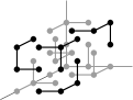
(b) $(3,2,2)$

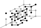
(c) $(4,2,2)$

(d) $(4,4,2)$

Figure 6. Non-defective pictures for some $(*,*,2)$.

Figure 6(a) gives a nice picture for $(d,e,f)=(2,2,2)$, The picture is defective, but it shows that $kX$ has the expected dimension for $k=1,\ldots,6$ and defect at most $1$ for $k=7$. From [5] we know that $7X$ is, indeed, defective, so we are done. Figure 6(b) gives a non-defective picture for $(3,2,2)$. Similarly, Figure 6(c) gives a non-defective picture for $(4,2,2)$.

Now let $d\geq 5$ and write $d+1=(3+1)q+(r+1)$ with $r\in\{1,3,4,6\}$. Then we can construct a non-defective picture for $(d,2,2)$ from $q$ non-defective pictures for $(3,2,2)$ and one non-defective picture for $(r,2,2)$. This settles $(d,2,2)$.

For $(2,3,2)$ and $(1,3,2)$ we have already found non-defective pictures. For $d\geq 3$ write $d+1=2q+(r+1)$ with $r\in\{1,2\}$. Then one can construct a non-defective picture for $(d,3,2)$ from $q$ non-defective pictures for $(1,3,2)$ and one non-defective picture for $(r,3,2)$. This settles $(d,3,2)$.

If $d+1$ is even, then we can a construct non-defective picture for $(d,e,2)$ with $d\geq e\geq 2$ as follows: write $e+1=2q+(r+1)$ with $r\in\{1,2\}$, and put together $q$ non-defective pictures for $(d,1,2)$ and one non-defective picture for $(d,r,2)$.

Figure 6(d) shows how a copy of our earlier non-defective picture for $(2,4,2)$ and a non-defective picture for $(1,4,2)$ can be put together to a non-defective picture for $(4,4,2)$. Now let $d\geq 6$ be even and write $d+1=4q+(r+1)$ with $r\in\{2,4\}$. Then one can construct a non-defective picture for $(d,4,2)$ from $q$ copies of our non-defective picture for $(3,4,2)$ and one non-defective picture for $(r,4,2)$.

This settles $(d,4,2)$.

Now suppose that $d\geq e\geq 5$ and $f=2$. Write $e+1=4*q+(r+1)$ with $r\in\{1,2,3,4\}$. Then we can construct a non-defective picture for $(d,e,2)$ from $q$ non-defective pictures for $(d,3,2)$ and one non-defective picture for $(d,r,2)$. This concludes the case where $d\geq e\geq f=2$.

Consider the case where $d\geq e\geq f=3$. This case is easy now: write, for instance, $e+1=q*2+(r+1)$ with $r\in\{1,2\}$. Then a non-defective picture for $(d,e,3)$ can be constructed from $q$ non-defective pictures for $(d,1,3)$ and one non-defective picture for $(d,r,3)$.

Figure 7. A non-defective picture for $(4,4,4)$.

The above gives (by rotating) non-defective pictures for $(d,e,4)$ for all $d\geq 1$ and $e\in\{1,2,3\}$. Figure 7 shows how to construct a non-defective picture for $(4,4,4)$. It may need a bit of explanation: the upper half is a non-defective picture for $(4,4,1)$, very close to that in Figure 5(c)—but the superflous pair of vertices is separated. The lower half is a non-defective picture for $(4,4,2)$, very close to that in Figure 6(d). By joining the lower one of the superflous vertices in the upper half with the triangle in the lower half, we create a non-defective picture for $(4,4,4)$. Now suppose that $d\geq e\geq 5$ and write $e+1=4q+(r+1)$ with $r\in\{1,2,3,4\}$. Then we find a non-defective picture for $(d,e,4)$ from $q$ non-defective pictures for $(d,3,4)$ and one non-defective picture for $(d,r,4)$.

Finally, suppose that $d\geq e\geq f\geq 5$, and write $f+1=4q+(r+1)$ with $r\in\{1,2,3,4\}$. Then a non-defective picture for $(d,e,f)$ can be assembled from $q$ non-defective pictures for $(d,e,3)$ and one non-defective picture for $(d,e,r)$. This concludes the proof of Theorem 1.3.

6. Secant dimensions of ${\mathbb{P}}^{2}\times{\mathbb{P}}^{1}$

For Theorem 1.3 we first deal with the defective cases: the Segre-Veronese embeddings of degree $(2,\text{even})$ are all defective by [9, Example 3.2]. That the embedding of degree $(3,1)$ is defective can be proved using a polynomial interpolation argument, used in [4] for proving defectiveness of other secant varieties: Split $(3,1)=(2,0)+(1,1)$. Now it is easy to see that given $5$ general points there exist non-zero forms $f_{1},f_{2}$ of multi-degrees $(2,0)$ and $(1,1)$, respectively, that vanish on those points. But then the product $f_{1}f_{2}$ vanishes on those points together with all its first-order derivatives; hence the $5$-th secant variety does not fill the space. The proof below shows that its codimension is not more than $1$.

For the non-defective proofs we have to solve the optimisation problems $\operatorname{AP}(B,k)$, where

$$B=\{(x,y,z)\in{\mathbb{Z}}^{3}\mid x,y,z\geq 0,x+y\leq d,\text{ and }z\leq e\}.$$

We will do a double induction over the degrees $e$ and $d$: First, in Subsections 6.1—6.4 we treat the cases where $e$ is fixed to $1,2,3,4$, respectively, by induction over $d$. Then, in Subsection 6.5 we perform the induction over $e$. We will always think of the $x$-axis as pointing towards the reader, the $y$-axis as pointing to the right and the $z$-axis as the vertical axis. By $T_{d,e}$ we will mean a picture (non-defective, if possible) for $(d,e)$. We will also use (non-defective) pictures from Section 5 as building blocks; we denote the picture for the Segre-Veronese embedding of ${\mathbb{P}}^{1}\times{\mathbb{P}}^{1}\times{\mathbb{P}}^{1}$ by of degree $(a,b,c)$ by $B_{a,b,c}$.

6.1. The cases where $e=1$

(a) $T_{1,1}$

(b) $T_{2,1}$

(c) $T_{3,1}$; defective

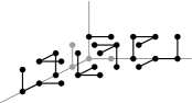
(d) $T_{4,1}$

Figure 8. Induction basis for $(*,1)$

Figures 8(a)–8(d) give pictures for $(d,1)$ with $d=1,\ldots,4$. Now we explain how to construct a non-defective picture for $(d+4,1)$ from a non-defective picture for $(d,1)$: First translate $T_{d,1}$ four steps to the right, and then proceed as follows:

1. If $d+1$ is even, $d+1=2l$ for some $l$, then put $l+1$ copies of $B_{1,3,1}$ to the left of $T_{d,1}$, starting at the origin. Finally, add a copy of $T_{2,1}$.

2. If $d+1$ is odd, $d+1=2l+1$ for some $l$, then put one copy of $B_{2,3,1}$ and $l-1$ copies of $B_{1,3,1}$ to the left of $T_{d,1}$. Finally, add another copy of $T_{2,1}$.

This is illustrated in Figure 9.

Figure 9. Induction step for $(*,1)$

To complete the induction, since $T_{3,1}$ is defective, we need a non-defective picture for $(7,1)$. We can construct this by using two copies of $T_{2,1}$, a box $B_{1,3,1}$ and the block $B_{2,2,1}$ (at the origin) from Figure 4(d). The remaining vertices are grouped together as in Figure 10 below.

Figure 10. Obtaining $T_{7,1}$

6.2. The cases where $e=2$

(a) $T_{1,2}$

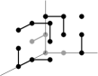
(b) $T_{2,2}$; defective

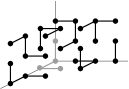
(c) $T_{3,2}$

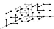
(d) $T_{4,2}$

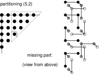
(e) $T_{5,2}$

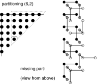
(f) $T_{6,2}$

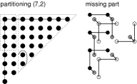
(g) $T_{7,2}$

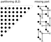
(h) $T_{8,2}$

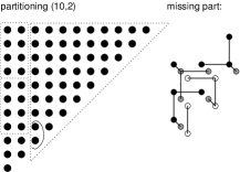
(i) $T_{10,2}$

Figure 11. Induction basis for $(*,2)$.

Figures 11(a)-11(i) lay the basis for the induction over $d$. Note that $T_{6,2}$ is the first among the pictures whose number of vertices is divisible by $4$. To finish the induction, we need to construct a non-defective picture for $(d+8,2)$ from $T_{d,2}$. First of all, move $T_{d,2}$ eight positions to the right. Then proceed as follows:

1. If $d$ is odd, $d=2l+1$ for some $l\geq 0$, put $l$ pairs of $B_{1,3,2}$ to the right of $T_{d,2}$ (starting at the origin), then two copies of $B_{2,3,2}$, and finally a copy of $T_{6,2}$.

2. If $d$ is even, $d=2l$ for some $l>0$, put $l+1$ pairs of $B_{1,3,2}$ starting at the origin. Finish off with one copy of $T_{6,2}$.

This is illustrated in Figure 12.

Figure 12. Induction step for $(*,2)$

6.3. The cases where $e=3$

(a) $T_{1,3}$

(b) $T_{2,3}$

Figure 13. Induction basis for $(*,3)$

Here the induction over $d$ is easier since every $T_{d,3}$ has its number of vertices divisible by $4$. Figures 13(a) and 13(b) lay the basis of the induction (the latter just consists of two copies of $T_{2,1}$). Now we show that from a non-defective $T_{d,3}$ with $d$ odd one can construct non-defective $T_{d+2,3}$ and $T_{d+3,3}$. Write $d=2l+1$, and proceed as follows.

1. Move $T_{2l+1,3}$ two positions to the right. Put a block $B_{2l+1,1,3}$ at the origin, and conclude with a copy of $T_{1,3}$. This gives $T_{2l+3,3}$.

2. Move $T_{2l+1,3}$ three steps to the right. Put a block $B_{2l+1,2,3}$ at the origin, and conclude with a copy of $T_{2,3}$.

For $d=3$ this is illustrated in Figure 14.

(a) odd $d+2$

(b) even $d+3$

Figure 14. Induction steps from $T_{3,3}$

6.4. The cases where $e=4$

(a) $T_{1,4}$

(b) $T_{2,4}$; defective

(c) $T_{3,4}$

(d) $T_{4,4}$

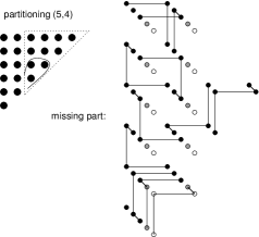
(e) $T_{5,4}$

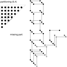
(f) $T_{6,4}$

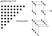
(g) $T_{7,4}$

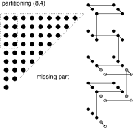
(h) $T_{8,4}$

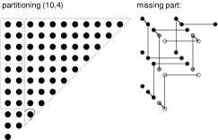
(i) $T_{10,4}$

Figure 15. Induction basis for $(*,4)$

Figures 15(a)-15(i) lay the basis of the induction. The induction step is identical to that where $e=2$, except that the blocks $B_{1,3,2}$ and $B_{2,3,2}$ have to be replaced by the blocks $B_{1,3,4}$ and $B_{2,3,4}$, and $T_{6,2}$ has to be replaced by $T_{6,4}$.

6.5. Induction over $e$

From a non-defective picture for $(d,e)$ we can construct a non-defective picture for $(d,e+4)$ by stacking a non-defective picture for $(d,3)$, whose number of vertices is divisible by $4$, on top of it. This settles all $(d,e)$ except for those that are modulo $(0,4)$ equal to the defective $(3,1)$ or $(2,2)$. The latter are easily handled, though: stacking copies of $T_{2,1}$ on top of $T_{2,2}$ gives pictures for all $(2,e)$ with $e$ even that are defective but give the correct, known, secant dimensions. So to finish our proof of Theorem 1.3 we only need the non-defective picture for $(3,5)$ of Figure 16.

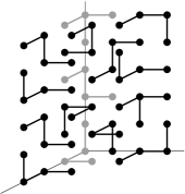
Figure 16. $T_{3,5}$

7. Secant dimensions of the point-line flag variety $\mathcal{F}$

In this section, $X=\mathcal{F}$, $G=\mathrm{SL}_{3}$, and the highest weight $\lambda$ equals $m\omega_{1}+n\omega_{2}$ with $m,n>0$. We first argue that $(m,n)=(1,1)$ and $(m,n)=(2,2)$ yield defective embeddings of $\mathcal{F}$. The first weight is the adjoint weight, so the cone $C_{1,1}$ over the image of $\mathcal{F}$ is just the set of rank-one, trace-zero matrices in $\mathfrak{sl}_{3}$, whose secant dimensions are well known. For the second weight let $C_{2,2}$ be the image of $C_{1,1}$ under the map $\mathfrak{sl}_{3}\rightarrow S^{2}(\mathfrak{sl}_{3}),v\mapsto v^{2}$. Then $C_{2,2}$ spans the $\mathrm{SL}_{3}$-submodule (of codimension $9$) in $S^{2}(\mathfrak{sl}_{3})$ of highest weight $2\omega_{1}+2\omega_{2}$, while it is contained in the quadratic Veronese embedding of $\mathfrak{sl}_{3}$. Viewing the elements of $S^{2}(\mathfrak{sl}_{3})$ as symmetric $8\times 8$-matrices, we find that $C_{2,2}$ consists of rank $1$ matrices, while it is not hard to prove that the module it spans contains matrices of full rank $8$. Hence $7C_{2,2}$ cannot fill the space.

For the non-defective proofs let $\alpha_{1},\alpha_{2}$ be the simple positive roots, so that ${X(\mathfrak{u})}=\{\beta_{1},\beta_{2},\beta_{3}\}$ with $\beta_{1}=-\alpha_{1}$, $\beta_{2}=-\alpha_{1}-\alpha_{2}$ and $\beta_{3}=-\alpha_{2}$. The subscripts indicate the order in which the PBW-monomials are computed: for $r=(n_{1},n_{2},n_{3})$ we write $m_{r}:=X_{\beta_{1}}^{n_{1}}X_{\beta_{2}}^{n_{2}}X_{\beta_{3}}^{n_{3}}v_{\lambda}$. Set

$$B:=\{(n_{1},n_{2},n_{3})\in{\mathbb{Z}}^{3}\mid 0\leq n_{2}\leq m,0\leq n_{3}\leq n,\text{ and }0\leq n_{1}\leq m+n_{3}-n_{2}\},$$

and let $M$ be the set of all $r\in{\mathbb{N}}^{{X(\mathfrak{u})}}$ with $m_{r}\neq 0$. We will not need $M$ explicitly; it suffices to observe that $r_{3}\leq n$ for all $r\in M$: indeed, if $r_{3}>n$ then $X_{\beta_{3}}^{r_{3}}v_{\lambda}$ is already $0$, hence so is $m_{r}$. We use the following consequence of the theory of canonical basis; see [6, Example 10, Lemma 11].

Lemma 7.1.

The $m_{b},b\in B$ form a basis of $V$.

Remark 7.2.

The map $(n_{1},n_{2},n_{3})\mapsto(n_{1},n-n_{3},m-n_{2})$ sends the set $B$, which corresponds on the highest weight $(m,n)$, to the set corresponding to the highest weight $(n,m)$. Hence if we have a non-defective picture for one, then we also have a non-defective picture for the other. We will use this fact occasionally.

We want to apply Lemma 2.4. First note that $r,r^{\prime}\in{\mathbb{R}}^{{X(\mathfrak{u})}}={\mathbb{R}}^{3}$ have the same weight if and only if $r-r^{\prime}$ is a scalar multiple of $z:=(1,-1,1)$. We set $r<r^{\prime}$ if and only if $r-r^{\prime}$ is a positive scalar multiple of $z$.

Lemma 7.3.

For all $r\in M\setminus B$ and all $b\in B$ with $\xi(b)=\xi(r)$ we have $b<r$, i.e., the difference $b-r$ is a positive scalar multiple of $z$.

Proof.

Suppose that $b=(n_{1},n_{2},n_{3})\in B$ and that $n_{3}<n$. Then the defining inequalities of $B$ show that $b+z=(n_{1}+1,n_{2}-1,n_{3}+1)$ also lies in $B$. This shows that $B$ is a lower ideal in $(M,\leq)$, i.e., if $b\in B$ and $r\in M$ with $r<b$, then also $r\in B$. This readily implies the lemma. ∎

Proposition 7.4.

$\operatorname{VP}(B,k)$ is a lower bound on $\dim kC$ for all $k$.

Proof.

This follows immediately from Lemma 2.4 and Lemma 7.3 when we take for $Z$ the one-dimensional cone ${\mathbb{R}}_{\geq 0}\cdot z$. ∎

(a) $(2,1)$

(b) $(2+2k,1)$

Figure 17. Pictures for $(\text{even},1)$.

In what follows we will assume that $m\geq n$ when convenient. We first prove, by induction over $m$ non-defectiveness for $(m,1)$ and $(m,2)$, and then do induction over $n$ to conclude the proof. Figure 18(a) for $(m,n)=(1,1)$ is not non-defective, reflecting that the adjoint minimal orbit—the cone over which is the cone of $3\times 3$-matrices with trace $0$ and rank $\leq 1$—is defective. Figure 17(a), however, shows a non-defective picture for $(2,1)$, and from this picture one can construct non-defective pictures for $(2+2k,1)$ by putting it to the right of $k$ pictures, each of which consists of cubes and a single tetrahedron; Figure 17(b) illustrates this for the step from $(2,1)$ to $(2+2,1)$.

(a) $(1,1)$; defective

(b) $(3,1)$

(c) $(5,1)$

(d) $(3+4k,1)$

Figure 18. Pictures for $(\text{odd},1)$

Figure 18(b) shows a non-defective picture for $(3,1)$, and Figure 18(c) a non-defective picture for $(5,1)$. From these we can construct non-defective pictures for $(3+4k,1)$ and $(5+4k,1)$, respectively, by putting them to the right of $k$ pictures, each of which consists of a few cubes plus a non-defective picture for $(3,1)$—Figure 18(d) illustrates this for the step from $(3,1)$ to $(7,1)$. This settles $(n,1)$.

(a) $(2,2)$; defective

(b) $(3,2)$

(c) $(4,2)$

(d) $(5,2)$

(e) $(6,2)$

(f) $(7,2)$

(g) $(m+8,2)$

Figure 19. Pictures for $(*,2)$

Figure 19(a) is defective: it reflects the fact that the $7$-th secant variety of $X$ in the $(2,2)$-embedding has defect $1$. Figure 19(b) gives a non-defective picture for $(3,2)$. Note that two non-standard cells $B_{i}$ are used here; this is because we will need this picture in the picture for $(6,6)$. Figure 19(c) gives a non-defective picture for $(4,2)$. One can construct a non-defective picture for $(5,2)$ based on the former, and a non-defective picture for $(7,2)$ based on that for $(4,2)$; see Figure 19(d) and Figure 19(f). In the latter picture, one should fill in one copy of our earlier non-defective picture for ${\mathbb{P}}^{1}\times{\mathbb{P}}^{1}\times{\mathbb{P}}^{1}$ in its $(3,2,2)$-embedding. Figure 19(e) gives a non-defective picture for $(6,2)$, based on that for $(4,2)$. A single cell $B_{i}$ is non-standard, again for later use in the picture for $(6,6)$. Similarly, one can construct pictures for $(8,2)$ and $(10,2)$—which are left out here because they take too much space.

Finally, from a non-defective picture for $(m,2)$ (with $m=1$ or $m\geq 3$) one can construct a non-defective picture for $(m+8,2)$ by inserting a picture consisting of a non-defective picture for $(7,2)$ and our non-defective picture for a $(7,m,2)$-block from the discussion of ${\mathbb{P}}^{1}\times{\mathbb{P}}^{1}\times{\mathbb{P}}^{1}$ in front—Figure 19(g) illustrates this for $m=1$. This settles the cases where $m\geq n=2$.

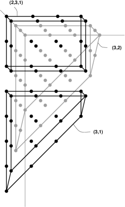
Figure 20. Construction for $m$ or $n$ odd.

Now all cases where at least one of $m$ and $n$ is odd can also be settled. Indeed, suppose that $m,n\geq 3$ and that $m$ is odd. Write $n+1=2q+(r+1)$ with $r\in\{1,2\}$. Then we can construct a non-defective picture for $(m,n)$ by taking our non-defective picture for $(m,r)$ and succesively stacking $q$ non-defective pictures of two layers on top, each of which pictures with a number of vertices divisible by $4$. These layers can be constructed as follows: the $i$-th layer consists of our non-defective picture for ${\mathbb{P}}^{1}\times{\mathbb{P}}^{1}\times{\mathbb{P}}^{1}$ with parameters $(r+2i-2,m,1)$ (lying against the $(n_{2},n_{3})$-plane) and a non-defective picture for $\mathcal{F}$ with parameters $(m,1)$. As $m$ is odd, each of these two blocks has a number of vertices divisible by $4$. This construction is illustrated for $m=3$ and $n=4$ in Figure 20, where one extra layer is put on top of the “ground layer”.

Only the cases remain where $m$ and $n$ are both even. We first argue that we can now reduce the discussion to a finite problem: if $m\geq 7$ and $n\geq 2$, then we can compose a non-defective picture for $(m,n)$ from one non-defective picture for $(7,n)$ (which exists by the above), one non-defective ${\mathbb{P}}^{1}\times{\mathbb{P}}^{1}\times{\mathbb{P}}^{1}$-picture for $(7,m-8,n)$ (both of these have numbers of vertices divisible by $4$), and one non-defective picture for $(m-8,n)$—if such a picture exists. Hence we may assume that $m<7$. Similarly, by using Remark 7.2 we may assume that $n<7$. Using that $m,n$ are even, and that $m,n>2$ (which we have already dealt with), we find that only $(4,4)$, $(4,6)$ (or $(6,4)$), and $(6,6)$ need to be settled—as done in Figures 21(a)–21(c). The picture for $(4,6)$ uses our picture for the Segre-Veronese embedding of ${\mathbb{P}}^{1}\times{\mathbb{P}}^{1}\times{\mathbb{P}}^{1}$ of degree $(5,1,4)$. The picture for $(6,6)$ is built from a picture for ${\mathbb{P}}^{1}\times{\mathbb{P}}^{1}\times{\mathbb{P}}^{1}$ of weight $(3,2,6)$, and pictures for $\mathcal{F}$ of weights $(2,6)$ and $(3,6)$; the latter picture, in turn, can be constructed as outlined above, except that, in order to line up the single edge in $(3,6)$ and the single vertex in $(2,6)$, the order of the building blocks for $(3,6)$ is altered: the $\mathcal{F}$-picture for $(3,2)$ comes on top, next to a $({\mathbb{P}}^{1})^{3}$ picture for $(3,3,1)$, and under these an $\mathcal{F}$-picture for $(3,3)$. This concludes the proof of Theorem 1.4.

(a) $(4,4)$

(b) $(4,6)$

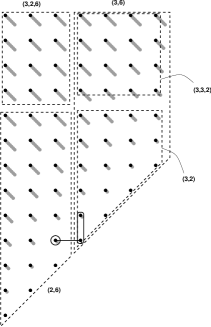
(c) $(6,6)$

References

- [1] J. Alexander and A. Hirschowitz. Polynomial interpolation in several variables. J. Algebr. Geom., 4(2):201–222, 1995.
- [2] Armand Borel. Linear Algebraic Groups. Springer-Verlag, New York, 1991.
- [3] Silvia Brannetti. Degenerazioni di varietà toriche e interpolazione polinomiale, 2007.
- [4] M.V. Catalisano, A.V. Geramita, and A. Gimigliano. Higher secant varieties of segre-veronese varieties. In C. et al. Ciliberto, editor, Projective varieties with unexpected properties. A volume in memory of Giuseppe Veronese. Proceedings of the international conference “Varieties with unexpected properties”, Siena, Italy, June 8–13, 2004, pages 81–107, Berlin, 2005. Walter de Gruyter.
- [5] M.V. Catalisano, A.V. Geramita, and A. Gimigliano. Segre-Veronese embeddings of and their secant varieties. Collect. Math., 58(1):1–24, 2007.
- [6] Willem A. de Graaf. Five constructions of representations of quantum groups. Note di Matematica, 22(1):27–48, 2003.
- [7] Mike Develin. Tropical secant varieties of linear spaces. Discrete Comput. Geom., 35(1):117–129, 2006.
- [8] Jan Draisma. A tropical approach to secant dimensions. J. Pure Appl. Algebra, 2007. To appear.
-
[9]
M.V.Catalisano, A.V.Geramita, and A.Gimigliano.
On the ideals of secant varieties to certain rational varieties.
2006.
Preprint, available from
http://arxiv.org/abs/math/0609054. - [10] Bernd Sturmfels and Seth Sullivant. Combinatorial secant varieties. Pure Appl. Math. Q., 2(3):867–891, 2006.