Cactus Framework: Black Holes to Gamma Ray Bursts

Abstract

Gamma Ray Bursts (GRBs) are intense narrowly-beamed flashes of $\gamma$-rays of cosmological origin. They are among the most scientifically interesting astrophysical systems, and the riddle concerning their central engines and emission mechanisms is one of the most complex and challenging problems of astrophysics today. In this article we outline our petascale approach to the GRB problem and discuss the computational toolkits and numerical codes that are currently in use and that will be scaled up to run on emerging petaflop scale computing platforms in the near future.

Petascale computing will require additional ingredients over conventional parallelism. We consider some of the challenges which will be caused by future petascale architectures, and discuss our plans for the future development of the Cactus framework and its applications to meet these challenges in order to profit from these new architectures.

I Current challenges in relativistic astrophysics and the Gamma-Ray Burst problem

Ninety years after Einstein first proposed his General Theory of Relativity (GR), astrophysicists are more than ever and in greater detail probing into regions of the universe where gravity is very strong and where, according to GR’s geometric description, the curvature of spacetime is large.

The realm of strong curvature is notoriously difficult to investigate with conventional observational astronomy, and some phenomena might bear no observable electro-magnetic signature at all and may only be visible in neutrinos (if sufficiently close to Earth) or in gravitational waves — ripples of spacetime itself which are predicted by Einstein’s GR. Gravitational waves have not been observed directly to date, but gravitational-wave detectors (e.g., LIGO lig , GEO geo , VIRGO vir ) are in the process of reaching sensitivities sufficiently high to observe interesting astrophysical phenomena.

Until gravitational-wave astronomy becomes reality, astrophysicists must rely on computationally and conceptually challenging large-scale numerical simulations in order to grasp the details of the energetic processes occurring in regions of strong curvature that are shrouded from direct observation in the electromagnetic spectrum by intervening matter or that have little or no electromagnetic signature at all. Such astrophysical systems and phenomena include the birth of neutron stars (NSs) or black holes (BHs) in collapsing evolved massive stars, coalescence of compact binary systems, gamma-ray bursts (GRBs), active galactic nuclei harboring supermassive black holes, pulsars, and quasi-periodically oscillating NSs (QPOs). In figure 1 we present example visualizations of binary BH and stellar collapse calculations carried out by our groups.

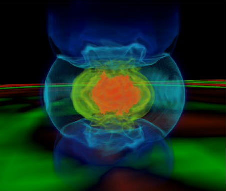
Figure 1: Left: Gravitational waves and horizons in a binary black hole inspiral simulation. Simulation by AEI/CCT collaboration, image by W. Benger (CCT/AEI/ZIB). Right: Rotationally deformed protoneutron star formed in the iron core collapse of an evolved massive star. Shown are a volume rendering of the rest-mass density and a 2D rendition of outgoing gravitational waves. Simulation by Ott et al. (2007), image by R. Kähler.

From these, GRBs, intense narrowly-beamed flashes of $\gamma$-rays of cosmological origin, are among the most scientifically interesting and the riddle concerning their central engines and emission mechanisms is one of the most complex and challenging problems of astrophysics today.

GRBs last between 0.5–1000 secs, with a bimodal distribution of durations Mészáros (2006), indicating two distinct classes of mechanisms and central engines. The short-hard (duration $\mathrel{\hbox{\raise 2.15277pt\hbox{$<$}\hbox to0.0pt{\hss\lower 2.15277pt\hbox{$\sim$}}}}2$ secs) group of GRBs (hard, because their $\gamma$-ray spectra peak at shorter wavelength) predominantly occurs in elliptical galaxies with old stellar populations at moderate astronomical distances Woosley and Bloom (2006); Mészáros (2006). The energy released in a short-hard GRB and its duration suggest Woosley and Bloom (2006); Mészáros (2006) a black hole with a $\sim$0.1 solar-mass ($\mathrm{M}_{\odot}$) accretion disk as the central engine. Such a BH–accretion-disk system is likely to be formed by the coalescence of NS–NS or NS–BH systems (e.g., Setiawan et al. (2006)).

Long-soft (duration $\sim$2–1000 secs) GRBs on the other hand seem to occur exclusively in the star-forming regions of spiral or irregular galaxies with young stellar populations and low metallicity Observations that have recently become available (see Mészáros (2006) for reviews) indicate features in the x-ray and optical afterglow spectra and luminosity evolutions of long-soft GRBs that show similarities with spectra and light curves obtained from Type-Ib/c core-collapse supernovae whose progenitors are evolved massive stars ($M\mathrel{\hbox{\raise 2.15277pt\hbox{$>$}\hbox to0.0pt{\hss\lower 2.15277pt\hbox{$\sim$}}}}25\,\mathrm{M}_{\odot}$) that have lost their extended hydrogen envelopes and probably also a fair fraction of their helium shell. These observations support the collapsar model Woosley and Bloom (2006) of long-soft GRBs that envisions a stellar-mass black hole formed in the aftermath of a stellar core-collapse event with a massive $\sim$1 $\mathrm{M}_{\odot}$ rotationally-supported accretion disk as the central engine, powering the GRB jet that punches through the compact and rotationally-evacuated polar stellar envelope reaching ultra-relativistic velocities Mészáros (2006).

Although observations are aiding our theoretical understanding, much that is said about the GRB central engine will remain speculation until it is possible to self-consistently model (i) the processes that lead to the formation of the GRB central engine and (ii) the way the central engine utilizes gravitational (accretion) and rotational energy to launch the GRB jet via magnetic stresses and/or polar neutrino pair-annihilation processes. The physics necessary in such a model includes general relativity, relativistic magneto-hydrodynamics, nuclear physics (describing nuclear reactions and the equation of state of dense matter), neutrino physics (weak interactions), and neutrino and photon radiation transport. In addition, it is necessary to adequately resolve physical processes with characteristic scales from $\sim$100 meters near the central engine to $\sim$5–10 million kilometers, the approximate radius of the collapsar progenitor star.

I.1 GRBs and petascale computing

The complexity of the GRB central engine and its environs requires a multi-physics, multi-length-scale approach that cannot be fully realized on present-day computers. Computing at multiple sustained petaflops of performance will allow us to tackle the full GRB problem and provide complete numerical models whose output can be compared with observations.

In this article we outline our petascale approach to the GRB problem and discuss the computational toolkits and numerical codes that are currently in use and that will be scaled up to run on emerging petaflop scale computing platforms in the near future.

Any comprehensive approach to GRBs must naturally draw techniques and tools from both numerical relativity and core-collapse supernova and neutron star theory. Hence, much of the work presented and suggested here builds upon the dramatic progress that has been made in these fields in the past decade. In numerical relativity, immense improvements in the long-term stability of 3D GR vacuum and hydrodynamics evolutions (e.g., Alcubierre et al. (2003); Pretorius (2005)) allow for the first time long-term stable binary black hole merger, binary neutron star merger, neutron star and evolved massive star collapse calculations. Supernova theory, on the other hand, has made giant leaps from spherically symmetric (1D) models with approximate neutrino radiation transport in the early 1990s, to Newtonian or approximate-GR to 2D and the first 3D Fryer and Warren (2004) calculations, including detailed neutrino and nuclear physics and energy-dependent multi-species Boltzmann neutrino transport Buras et al. (2006) or neutrino flux-limited diffusion Burrows et al. (2007a) and magneto-hydrodynamics Burrows et al. (2007b).

As we shall discuss, our present suite of terascale codes, comprised of the spacetime evolution code Ccatie and the GR hydrodynamics code Whisky can be and has already been applied to the realistic modeling of the inspiral and merger phase of NS–NS and NS-BH binaries, to the collapse of polytropic (cold) supermassive NSs, and to the collapse and early post-bounce phase of a core-collapse supernova or a collapsar. As the codes will be upgraded and readied for petascale, the remaining physics modules will be developed and integrated. In particular, energy-dependent neutrino transport and magneto-hydrodynamics, both likely to be crucial for the GRB central engine, will be given high priority.

To estimate roughly the petaflopage and petabyteage required for a full collapsar-type GRB calculation, we assume a Berger-Oliger-type Berger and Oliger (1984) adaptive-mesh refinement setup with 16 refinement levels, resolving features with resolution of 10,000 km down to 100 m across a domain of 5 million cubic km. To simplify things, we assume that each level of refinement has twice the resolution as the previous level and covers approximately half the domain. Taking a base grid size of 1024³ and 512 3D grid functions, storing the curvature, and radiation-hydrodynamics data on each level, we estimate a total memory consumption of $\sim$0.0625 PB (64 TB). To obtain an estimate of the required sustained petaflopage, we first compute the number of time steps that are necessary to evolve for 100 s in physical time. Assuming a time step that is half the light-crossing time of each grid cell on each individual level, the base grid has to be evolved for $\sim$6000 time steps, while the finest grid will have to be evolved for $2^{16-1}\times 6000$ individual time steps. Ccatie plus Whisky require approximately 10k flops grid point per time step. When we assume that additional physics (neutrino and photon radiation transport, magnetic fields; some of which may be evolved with different and varying time step sizes) requires on average additional 22k flops, one time step of one refinement level requires $10^{-5}$ petaflops. Summing up over all levels and time steps, we arrive at a total petaflopage of $\sim$13 million. On a machine with 2 petaflops sustained, the runtime of the simulation would come to $\sim$75 days. GRBs pose a true petascale problem.

II The Cactus framework

To reduce the development time for creating simulation codes and encourage code reuse, researchers have created computational frameworks such as the Cactus Framework Goodale et al. (2003); cac . Such modular component-based frameworks allow scientists and engineers to develop their own application modules (CS services or physics solvers) and assemble them with a body of existing code components to create applications that solve complex multiphysics computational problems. Cactus provides tools ranging from basic computational building blocks to complete toolkits that can be used to solve a range of application problems. Cactus runs on a wide range of hardware ranging from desktop PC’s, large supercomputers, to ’grid’ environments. The Cactus Framework and core toolkits are distributed with an open source license from the Cactus website cac , are fully documented, and are maintained by active developer and user communities.

The Cactus Framework consists of a central infrastructure (“flesh”) and components (“thorns”). The flesh has minimal computational functionality and serves as a module manager, coordinating the flow of data between the different components to perform specific tasks. The components or “thorns” perform tasks ranging from setting up a computational grid, decomposing the grid for parallel processing, setting up coordinate systems, boundary and initial conditions, communication of data from one processor to another, solving partial differential equations, to input and output and streaming of visualization data. One standard set of thorns is distributed as the Cactus Computational Toolkit to provide basic functionality for computational science.

Cactus was originally designed for scientists and engineers to collaboratively develop large-scale, parallel scientific codes which would be run on laptops and workstations (for development) and large supercomputers (for production runs). The Cactus thorns are organized in a manner that provides a clear separation of the roles and responsibilities between the “expert computer scientists” who implement complex parallel abstractions (typically in C or C++), and the “expert mathematicians and physicists” who program thorns that look like serial blocks of code (typically, in F77, F90, or C) implementing complex numerical algorithms. Cactus provides the basic parallel framework supporting several different codes in the numerical relativity community used for modeling black holes, neutron and boson stars and gravitational waves. This has lead to over 150 scientific publications in numerical relativity which have used Cactus and the establishment of a Cactus Einstein Toolkit of shared community thorns. Other fields of science and engineering are also using the Cactus Framework, including Quantum Gravity, Computation Fluid Dynamics, Computational Biology, Coastal Modeling, Applied Mathematics etc, and in some of these areas community toolkits and shared domain specific tools and interfaces are emerging.

Cactus provides a range of advanced development and runtime tools including; an HTTPD thorn that incorporates a simplified web server into the simulation allowing for real-time monitoring and steering through any web interface; a general timer infrastructure for users to easily profile and optimize their codes; visualization readers and writers for scientific visualization packages; and interfaces to Grid Application Toolkits for developing new scientific scenarios taking advantage of distributed computing resources.

Cactus is highly portable. Its build system detects differences in machine architecture and compiler features, using automatic detection where possible and a database of known system environments where auto-detection is impractical — e.g. which libraries are necessary to link Fortran and C code together for a particular system architecture or facility. Cactus runs on nearly all variants of the Unix operating system, Windows platform, and a number of microkernels including Catamount and BlueGene CNK. Codes written using Cactus have been run on some of the fastest computers in the world, such as the Japanese Earth Simulator and the IBM BlueGene/L, Cray X1e, and the Cray XT3/XT4 systems Oliker et al. (Mar 26-30, 2007, 2003, Nov6-12, 2004); Carter et al. (July 10-12, 2006); Kamil et al. (2005); Shalf et al. (Nov 12-18, 2005) Cactus’ flexible and robust build system enables developers to write and test code on their laptop computers, and then deploy the very same code on the full scale systems with very little effort.

III Spacetime and hydrodynamics codes

III.1 Ccatie: Spacetime evolution

In strong gravitational fields, such as in the presence of neutron stars or black holes, it is necessary to solve the full Einstein equations. Our code employs a $3+1$ decomposition Arnowitt et al. (1962); York (1979), which renders the four-dimensional spacetime equations into hyperbolic time-evolution equations in three dimensions, plus a set of constraint equations which have to be satisfied by the initial condition. The equations are discretized using high order finite differences with adaptive mesh refinement and using Runge–Kutta time integrators, as described below.

The time evolution equations are formulated using a variant of the BSSN formulation described in Alcubierre et al. (2000) and coordinate conditions described in Alcubierre et al. (2003) and van Meter et al. (2006). These are a set of $25$ coupled partial differential equations which are first order in time and second order in space. One central variable describing the geometry is the three-metric $\gamma_{ij}$, which is a symmetric positive definite tensor defined everywhere in space, defining a scalar product which defines distances and angles.

Ccatie contains the formulation and discretization of the right hand sides of the time evolution equations. Initial data and many analysis tools, as well as time integration and parallelisation, are handled by other thorns. The current state of the time evolution, i.e., the three-metric $\gamma_{ij}$ and related variables, are communicated into and out of Ccatie using a standard set of variables (which is different from Ccatie’s evolved variables), which makes it possible to combine unrelated initial data solvers and analysis tools with Ccatie, or to replace Ccatie by other evolution methods, while reusing all other thorns.

A variety of initial conditions are provided by the Ccatie thorn, ranging from simple test cases, analytically known and perturbative solutions to binary systems containing neutron stars and black holes.

The numerical kernel of Ccatie has been hand-coded and extensively optimised for FPU performance where the greatest part of the computation lies. (Some analysis methods can be similarly expensive and have been similarly optimised, e.g. the calculation of gravitational wave quantities.) The Cactus/Ccatie combination has won various awards for performance.

III.2 Whisky: General relativistic hydrodynamics

The Whisky code Baiotti et al. (2005); whi is a GR hydrodynamics code originally developed under the auspices of the European Union research training network “Sources of Gravitational Waves” eun .

While Ccatie in combination with Cactus’s time-integration methods provides the time evolution of the curvature part of spacetime, Whisky evolves the “right-hand side”, the matter part, of the Einstein equations. The coupling of curvature with matter is handled by Cactus via a transparent and generic interface, providing for modularity and interchangeability of curvature and matter evolution methods. Whisky is also fully integrated with the Carpet mesh refinement driver discussed in §IV.2.

Whisky implements the equations of GR hydrodynamics in a semi-discrete fashion, discretising only in space and leaving the explicit time integration to Cactus. The update terms for the hydrodynamic variables are computed via flux-conservative finite-volume methods exploiting the characteristic structure of the equations of GR hydrodynamics. Multiple dimensions are handled via directional splitting. Fluxes are computed via piecewise-parabolic cell-interface reconstruction and approximate Riemann solvers to provide right-hand side data that are accurate to (locally) third-order in space and first-order in time. High temporal accuracy is obtained via Runge-Kutta-type time-integration cycles handled by Cactus.

Whisky has found extensive use in the study of neutron star collapse to a black hole, incorporates matter excision techniques for stable non-vacuum BH evolutions, has been applied to BH – NS systems, and NS rotational instabilities.

In a recent upgrade, Whisky has been endowed with the capability to handle realistic finite-temperature nuclear equations of state and to approximate the effects of electron capture on free protons and heavy nuclei in the collapse phase of core-collapse supernovae and/or collapsars Ott et al. (2007). In addition, a magneto-hydrodynamics version of Whisky, WhiskyMHD, is approaching the production stage Giacomazzo and Rezzolla (2007).

IV Parallel implementation and mesh refinement

In Cactus, infrastructure components providing storage handling, parallelisation, mesh refinement, and I/O methods are implemented by thorns in the same manner that numerical components provide boundary conditions or physics components provide initial data. The component which defines the order in which the time evolution is orchestrated, and implements the parallel execution model is called the driver.

Cactus has generally been used to date for calculations based upon explicit finite difference methods. Each simulation routine is invoked with a block of data — e.g. in a 3-dimensional simulation the routine is passed a cuboid, in a 2-dimensional simulation a rectangle — and integrates the data in this block forward in time. In general, the simulation routines only operate on the data they are handed (no side-effects), do not carry any internal state between invocations (statelessness), and do not directly control the order of execution (they merely define constraints on orderings). This organizes the Fortran and C (declarative) modules in a manner that is very similar to functional/imperative constraints. The imperative scheduling model provides the Cactus drivers considerable flexibility for the scheduling parallel execution. Consequently, Cactus supports a number of execution paradigms (offered by different driver) without requiring any changes to the physics modules to accommodate them.

For example, in a single processor simulation the block would consist of all the data for the whole of the simulation domain, and in a multi-processor simulation the domain is decomposed into smaller subdomains, where each processor computes the block of data from its subdomain. In a finite difference calculation, the main form of communication between these subdomains is on the boundaries, and this is done by ghost-zone exchange whereby each subdomain’s data-block is enlarged by the nearest boundary data from neighbouring blocks. The data from these ghost-zones is then exchanged once per iteration of the simulation. Cactus can also support shared-memory, out-of-core, and AMR execution paradigms through different drivers while still using the very same physics components.

There are several drivers available for Cactus. In this paper we present results using the unigrid PUGH driver and using the adaptive mesh refinement (AMR) driver Carpet.

IV.1 PUGH

The Parallel UniGrid Hierarchy (PUGH) driver was the first parallel driver available in Cactus. PUGH decomposes the problem domain into one block per processor using MPI for the ghost-zone exchange described above. PUGH has been successfully used on many architectures and has proven scaling up to many thousands of processors Oliker et al. (Mar 26-30, 2007). Figure 2 shows benchmark results from BlueGene/L. (See also figure 6 in the chapter “Performance Characteristics of Potential Petascale Scientific Applications” by Oliker et al.)

Figure 2: PUGH scaling result from BlueGene/L. (See also figure 6 in the chapter “Performance Characteristics of Potential Petascale Scientific Applications” by Oliker et al. for similar Cactus/PUGH benchmarks.)

IV.2 Adaptive Mesh Refinement with Carpet

Carpet Schnetter et al. (2004); car is a driver which implements Berger–Oliger mesh refinement Berger and Oliger (1984). Carpet refines parts of the simulation domain in space and/or time by factors of two. Each refined region is block-structured, which allows for efficient representations e.g. as Fortran arrays.

In addition to mesh refinement, Carpet also provides parallelism by distributing grid functions onto processors, corresponding I/O methods for ASCII and HDF5 output and for checkpointing and restart, interpolation of values to arbitrary points, and reduction operations such as norms and maxima.

Fine grid boundary conditions require interpolation in space. This is currently implemented up to seventh order, and fifth order is commonly used. When refining in time, finer grids take smaller time steps to satisfy the local CFL criterion. In this case, Carpet may need to interpolate coarse grid data in time to provide boundary conditions for fine grids. Similarly, time interpolation may also be required for interpolation or reduction operations at times when no coarse grid data exist. Such time interpolation is currently implemented with up to fourth order accuracy, although only second order is commonly used.

In order to achieve convergence at mesh refinement boundaries when second spatial derivatives appear in the time evolution equations, we do not apply boundary conditions during the substeps of a Runge–Kutta time integrator. Instead we extend the refined region by a certain number of grid points before each time step (called buffer zones) and only interpolate after each complete time step. We find that this is not necessary when no second derivatives are present, such as in discretisations of the Euler equations without the Einstein equations. The details of this algorithm are laid out in Schnetter et al. (2004).

Carpet is currently mostly used in situations where compact objects need to be resolved in a large domain, and Carpet’s mesh refinement adaptivity is tailored for these applications. One can define several centres of interest, and space will be refined around these. This is ideal e.g. for simulating binary systems, but is not well suited for resolving shock fronts as they e.g. appear in collapse scenarios. We plan to address this soon in future versions of Carpet.

IV.3 I/O

Our I/O methods are based on the HDF5 hdf library, which provides a platform-independent high-performance file parallel format. Datasets are annotated with Cactus-specific descriptive attributes providing meta-data e.g. for the coordinate systems, tensor types, or the mesh refinement hierarchy.

Some file systems can only achieve high performance when each processor or node writes its own file. However, writing one-file-per-processor on massively concurrent systems will be bottlenecked by the metadata server, which often limits file-creation rates to only hundreds of files per second. Furthermore, creation of many thousands of files can create considerable metadata management headaches. Therefore the most efficient output setup is typically to designate every $n$th processor as output processor, which collects data from $n-1$ other processors and writes the data into a file.

Input performance is also important when restarting from a checkpoint. We currently use an algorithm where each processor reads data only for itself, trying to minimise the number of input file which it examines.

Cactus also supports novel server-directed I/O methods such as PANDA, and other I/O file formats such as SDF and FlexIO. All of these I/O methods are interchangeable modules that can be selected by the user at compile-time or runtime depending on their needs and local performance characteristics of the cluster file systems. This makes it very easy to provide head-to-head comparisons between different I/O subsystem implementations that are nominally writing out exactly the same data.

V Scaling on current machines

We have evaluated the performance of the kernels of our applications on various contemporary machines to establish the current state of the code. This is part of an ongoing effort to continually adapt the code to new architectures. These benchmark kernels include the time evolution methods of Ccatie with and without Whisky, using as driver either PUGH or Carpet. We present some recent benchmarking result below; we list the benchmarks in table 1 and the machines and their characteristics in table 2.

Table 1: Our benchmarks and their characteristics. The PUGH and Carpet_1lev benchmarks evolve the vacuum Einstein equations without mesh refinement, with identical setups but using different communication strategies. Carpet_8lev features 8 fixed levels with the same number of grid points on each level. Whisky_8lev evolves the relativistic Euler equations in addition to the Einstein equations. BenchIO_HDF5_80l writes several large files to disk using the Cactus checkpointing facility.

Name	type	complexity	physics
Bench_Ccatie_PUGH	compute	unigrid	vacuum
Bench_Ccatie_Carpet_1lev	compute	unigrid	vacuum
Bench_Ccatie_Carpet_8lev	compute	AMR	vacuum
Bench_Ccatie_Whisky_Carpet	compute	AMR	hydro
BenchIO_HDF5_80l	I/O	unigrid	vacuum

Table 2: The machines used for the benchmarks in this section. Note that we speak of “processes” as defined in the MPI standard; these are implicitly mapped onto the hardware “cores” or “CPUs”.

Name	Host	CPU	ISA	Interconnect	# proc	cores/	cores/	memory/	CPU freq.
						node	socket	proc
Abe	NCSA	Clovertown	x86-64	InfiniBand	9600	8	4	1 GByte	2.30 GHz
Damiana	AEI	Woodcrest	x86-64	InfiniBand	672	4	2	2 GByte	3.00 GHz
Eric	LONI	Woodcrest	x86-64	InfiniBand	512	4	2	1 GByte	2.33 GHz
Pelican	LSU	Power5+	PPC64	Federation	128	16	2	2 GByte	1.90 GHz
Peyote	AEI	Xeon	x86-32	GigaBit	256	2	1	1 GByte	2.80 GHz

Since the performance of the computational kernel does not depend on the data which are evolved, we choose trivial initial data for our spacetime simulations, namely the Minkowski spacetime (i.e., vacuum). We perform no analysis on the results and perform no output. We choose our resolution such that approximately 800 MByte of main memory is used per process, since we presume that this makes efficient use of a node’s memory without leading to swapping. We run the simulation for several time steps requiring several wall-time minutes. We increase the number of grid points with the number of processes. We note that the typical usage model for this code favors weak scaling as resolution of the computational mesh is a major limiting factor for accurate modeling of the most demanding problems.

Our benchmark source code, configurations, parameter files, and detailed benchmarking instruction are available from the Cactus web site cac . There we also present results for other benchmarks and machines.

V.1 Floating point performance

Figure 3 compares the scaling performance of our code on different machines. The graphs show scaling results calculated from the wall time for the whole simulation, but excluding startup and shutdown. The ideal result in all graphs is a straight horizontal line, and larger numbers are better. Values near zero indicate lack of scaling.

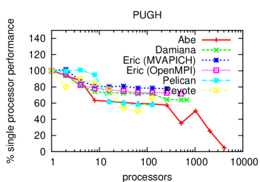
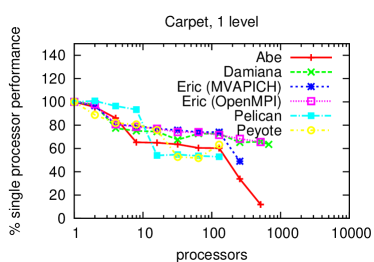
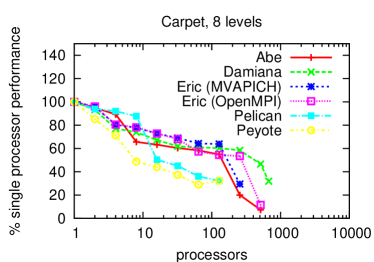
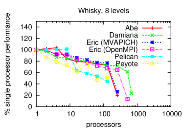
Figure 3: Weak scaling tests using our four benchmarks on various machines. The graphs show the fraction of single processor performance which is achieved on multiple processors. The PUGH and 1lev benchmarks have identical setups, but use different drivers with different communication strategies. On Eric, we also compare two different MPI implementations.

Since the benchmarks Bench_Ccatie_PUGH and Bench_Ccatie_Carpet_1lev use identical setups, they should ideally also exhibit the same scaling behaviour. However, as the graphs show, PUGH scales e.g. up to 1024 processors on Abe, while Carpet scales only up to 128 processors on the same machine. The differences are caused by the different communication strategies used by PUGH and Carpet, and likely also by the different internal bookkeeping mechanisms. Since Carpet is a mesh refinement driver, there is some additional internal overhead (not communication overhead), even in unigrid simulations.

Both PUGH and Carpet use MPI_Irecv MPI_Isend, and MPI_Wait to exchange data asynchronously. PUGH exchanges ghost zone information in 3 sequential steps, first in the $x$, then in the $y$, and then in the $z$ direction. In each step, each processor communicates with two of its neighbours. Carpet exchanges ghost zone information in a single step, where each processor has to communicate with all 26 neighbours. In principle, Carpet’s algorithm should be more efficient, since it does not contain several sequential steps; in practice, performance suffers because it sends are larger number of small messages than PUGH. The overhead of sending small messages has a marked impact on performance. A lighter-weight communication mechanism such as one-sided messages may provide significant benefits to future implementations of Carpet.

The fall-off at small processor numbers coincides with the node boundaries. For example, Abe drops off at the 8-processor boundary, and Pelican drops off at the 16-processor boundary. This is most likely because a fully loaded node provides less memory bandwidth to each process.

The scaling drop-off at large processor numbers for the commodity clusters appears to be caused by dramatic growth in memory usage by MPI implementations as the concurrency of the simulation is scaled up. This drop-off is different for different MPI implementations, as is e.g. evident on Eric, where OpenMPI scales further than MVAPICH. As the memory footprint grows, there is additional TLB thrashing – particularly on the Opteron processors, which have a comparatively small TLB coverage of 2MB when using small pages. So it may only take a 1% miss rate to have a dramatic effect on performance. Large pages seem to not offer a performance advantage.

However, we saw now such growth in memory consumption on the BlueGene/L system, which was able to scale up to 32k processors with little degradation as shown in figure 2. The BlueGene/L scaling study shows that by using a MPI implementation that does not grow with concurrency, Cactus can continue to scale up to phenomenal concurrencies with little drop-off in performance.

V.2 I/O performance

Figure 4 compares the scaling of different I/O methods: Collecting the output onto a single processor, having every $n$th processor perform output, and outputting on every processor. Each output processor creates one file. In these benchmarks, for each compute processor 369 MByte need to be written to disk. There is a small additional overhead per generated file which is less than 1 MByte.

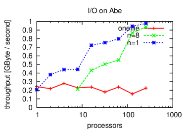
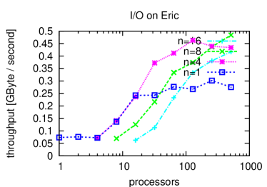
Figure 4: I/O scaling on various machines. This benchmark was only run on Abe and Eric. For each processor, 369 MByte of data are written to disk.

The throughput graphs of Abe and Eric show that the maximum single-node throughput is limited, but the overall throughput can be increased if multiple nodes write simultaneously. While Abe has sufficient bandwidth to support every CPU writing at the same time, it is more efficient on Eric to collect the data first onto fewer processors.

VI Developing for petascale

Petascale computing requires additional ingredients over conventional parallelism. The large number of available processors can only be fully exploited with mechanisms for significantly more fine-grained parallelism, in particular more fine grained than offered by the MPI standard’s collective communication calls. In order to ensure correctness in the presence of more complex codes and of increasingly likely hardware failures, simulations should be divided into parcels describing a certain amount of computation. These parcels of computation can then be autonomously and dynamically distributed over the available cores on the system by the Cactus driver, and can be re-scheduled in response to hardware failure, thus achieving both load balancing and end-to-end correctness, akin to the way the IP protocol is used to deliver reliability over unreliable components. Furthermore, the current static simulation schedule — often described by a sequence of subroutine calls — needs to become dynamic. The latter can be achieved e.g. by listing pre- and postconditions of each substep, and determining an efficient execution order only at run time, akin to the way UNIX make functions. The fact that Cactus physics modules are written with the same rules as operators in functional languages (namely that they are stateless and have no side-effects), enables this kind of flexibility in scheduling that will be necessary to carry us beyond the Petascale systems.

Clearly, these are only some measures, and a reliable methodology for petascale computing requires a comprehensive set of concepts which enable and encourage the corresponding algorithms and programming styles. It will very likely be necessary to develop new algorithms for petascale machines. These algorithms may not necessarily run efficiently on single processors or today’s popular small workstation clusters, in the same way in which vectorised codes do not work well on non-vector machines, or in which MPI codes may not work well on single-processor machines.

One example of a non-petascale parallelisation algorithm which is currently widely employed is the use of ghost zones to distribute arrays onto multiple processors. As the number of processors increases, each processor receives a correspondingly smaller part of the original array, while the overhead (the ratio between the number of ghost zones to the number of owned points) increases. Some typical numbers illustrate this: Our fourth-order stencils require a ghost zone layer which is $3$ points wide. If a processor owns $20^{3}$ grid points of a 3D array, the overhead is $(26^{3}-20^{3})/20^{3}\approx 20\%$. If a processor owns only $10^{3}$ grid points, then the overhead increases to $(16^{3}-10^{3})/10^{3}\approx 310\%$: the number of ghost zones is more than three times the number of owned points. Clearly we cannot continue to scale this approach in its current form.

Another problem for petascale simulations is time integration, i.e., the solution of hyperbolic equations. Since each time step depends on the result of the previous time step, time integration is inherently serial. If a million time steps are required, the total time to solution is at least a million times the time for a single time step.

The Cactus framework with its clear division between physical calculations and computational infrastructure already provides a partial pathway to petascale computations. By improving or exchanging the driver, existing physics modules can be used in novel ways, e.g. invoking them on smaller parts of the domain, or scheduling several at the same time to overlap computation and communication. Such improvement would be very difficult without a computational framework. However, achieving full petascale performance will also require improvements to the framework itself, i.e., to the way in which a physics calculation describes itself and its interface to the framework.

VI.1 Physics: radiation transport

The most conceptually and technically challenging part of the petascale development will be related to the implementation of neutrino and photon radiation transport. While photons play an important role in the jet propagation and, naturally, in the gamma-ray emission of the GRB, neutrinos are of paramount importance in the genesis and evolution of the GRB engine, in particular in the collapsar context. During the initial gravitational collapse to a protoneutron star and in the latter’s short cooling period before black hole formation, neutrinos carry away $\sim$99% of the liberated gravitational binding energy. After black-hole formation, neutrino-cooling of the accretion disk and polar neutrino-antineutrino pair-annihilation are likely to be key ingredients for the GRB mechanism.

Ideally, the neutrino radiation field should be described and evolved via the Boltzmann equation, making the transport problem 7-dimensional and requiring the inversion of a gigantic semi-sparse matrix at each time step. This matrix inversion will be at the heart of the difficulties associated with the parallel scaling of radiation transport algorithms and it is likely that even highly-integrated low-latency petascale systems will not suffice for full Boltzmann radiation transport, and sensible approximations will have to be worked out and implemented.

One such approximation may be neutrino, multi-energy-group,flux-limited diffusion (MGFLD) along individual radial rays that are not coupled with each other and whose ensemble covers the entire sphere/grid with reasonable resolution of a few degrees. When in addition energy-bin coupling (downscattering of neutrinos, a less-than-10%-effect) and neutrino flavor changes are neglected, each ray for each energy group can be treated as a mono-energetic spherically symmetric calculation. Each of these rays can then be domain decomposed, and the entire ensemble of rays and energy groups can be updated in massively-parallel and entirely scalable petascale fashion.

A clear downside of MGFLD is that all local angular dependence of the radiation field is neglected, making it (for example) fundamentally difficult to consistently estimate the energy deposited by radiation-momentum angle-dependent neutrino-antineutrino annihilation. An alternative to the MGFLD approximation that can provide an exact solution to the Boltzmann transport equation, while maintaining scalability, is the statistical Monte Carlo approach that follows a significant set of sample particle random walks. Monte Carlo may also be the method of choice for photon transport.

VI.2 Scalability

In its current incarnation, the Cactus framework and its drivers PUGH and Carpet are not yet fully ready for petascale applications. Typical petascale machines will have many more processing units than today’s machines, with more processing units per node, but likely with less memory per processing unit.

One immediate consequence is that it will be impossible to replicate metadata across all processors. Not only the simulation data themselves, but also all secondary data structures will need to be distributed, and will have to allow asynchronous remote access. The driver thorns will have to be adapted to function without global knowledge of the simulation state, communicating only between neighbouring processors, making global load balancing a challenge.

The larger number of cores per node will make hybrid communication schemes feasible and necessary, where intra-node communication uses shared memory while inter-node communication remains message based. Explicit or implicit multithreading within a node will reduce the memory requirements, since data structures are kept only once per node, but will require a more complex overall orchestration to keep all threads well fed. Multithreading will have direct consequences for and may require alterations to almost all existing components. Multithreading will required a change of programming paradigm, as programmers will have to avoid race conditions, and debugging will be much more difficult than for a single-threaded code.

With the increasing number of nodes, globally synchronous operations will become prohibitively expensive, and thus the notion of “the current simulation time” will need to be abolished. Instead of explicitly stepping a simulation through time, different parts will advance at different speeds. Currently global operations, such as reduction or interpolation operations, will need to be broken up into hierarchical pieces which are potentially executed at different times, where the framework has to ensure that these operations find the corresponding data, and that result of such operations are collected back where they were requested.

Current Cactus thorns often combine the physics equations which are to be solved and the discretisation methods used to implement them, e.g. finite differences on block-structured grids. Petascale computing may require different discretisation techniques, and it will thus be necessary to isolate equations from their discretisation so that one can be changed while keeping the other. Automated code generation tools such as e.g. Kranc Husa et al. (2006); kra can automatically generate physics modules from given equations, achieving this independence.

As a framework, Cactus will not implement solutions to these problems directly, but will instead provide abstractions which can be implemented by a variety of codes. As external AMR drivers mature and prove themselves, they can be connected into Cactus. We are currently engaged in projects to incorporate the PARAMESH par ; MacNeice et al. (2000) and SAMRAI sam AMR infrastructures into Cactus drivers in the projects Parca (funded by NASA) and Taka, respectively.

Instead of continuing to base drivers on MPI, we plan to investigate existing new languages such as e.g. co-array Fortran, Titanium, and UPC to provide parallelism, while we will also examine novel parallel computing paradigms such as ParalleX. Cactus will be able to abstract most of the differences between these, so that the same physics and/or numerics components can be used with different drivers.

It should be noted that the Cactus framework does not prescribe a particular computing model. For example, after introducing AMR capabilities into Cactus, most existing unigrid thorns could be AMRified with relatively little work; the existing abstraction that each routine works on a block-structured set of grid point was sufficient to enable the introduction of mesh refinement. We expect that the existing abstractions will need to be updated for petascale computing, containing e.g. information about simultaneous action of different threads and removing the notion of a global simulation time, but we also expect that this same abstraction will then cover a multitude of possible petascale computing models.

VI.3 Tools

Petascale computing provides not only new challenges for programming methodologies, but will also require new tools to enable programmers to cope with the new hardware and software infrastructure. Debugging on $100,000+$ processors will be a formidable challenge, and only good and meaningful profiling information for the new dynamic algorithms will make petascale performance possible. These issues are being addressed in three NSF-funded projects.

In the ALPACA (Application Level Profiling And Correctness Analysis) project, we are developing interactive tools to debug and profile scientific applications at the petascale level. When a code has left the stage where it has segmentation faults, it is still very far from giving correct physical answers. We plan to provide debuggers and profilers which will not examine the programme from the outside, but will run together with the programme, being coupled to the programme via the framework, so that it has first-class information about the current state of the simulation. We envision a smooth transition between debugging and watching a production run progressing, or between running a special benchmark and collecting profiling information from production runs on the side.

The high cost of petascale simulations will make it necessary to treat simulation results similar to data gathered in expensive experiments. Our XiRel (CyberInfrastructure for Numerical Relativity) project seeks to provide scalable adaptive mesh refinement on one hand, but also to provide means to describe and annotate simulation results, so that these results can later be interpreted and analysed unambiguously and that the provenance of these data remains clear. With ever increasing hardware and software complexity, ensuring reproducibility of numerical results is becoming an important part of scientific integrity.

The DynaCode project is providing capabilities and tools to adapt and respond to changes in the computational environment, such as e.g. hardware failures, changes in the memory requirement of the simulation, or user-generated requests for additional analysis or visualisation. This will include interoperability with other frameworks.

References

- (1) LIGO: Laser Interferometer Gravitational Wave Observatory, URL http://www.ligo.caltech.edu/.
- (2) GEO 600, URL http://www.geo600.uni-hannover.de/.
- (3) VIRGO, URL http://www.virgo.infn.it/.
- Ott et al. (2007) C. D. Ott, H. Dimmelmeier, A. Marek, H. . Janka, I. Hawke, B. Zink, and E. Schnetter, Phys. Rev. Lett. in press (2007), eprint astro-ph/0609819.
- Mészáros (2006) P. Mészáros, Reports of Progress in Physics 69, 2259 (2006), eprint astro-ph/0605208.
- Woosley and Bloom (2006) S. E. Woosley and J. S. Bloom, Ann. Rev. Astron. Astrophys. 44, 507 (2006), eprint astro-ph/0609142.
- Setiawan et al. (2006) S. Setiawan, M. Ruffert, and H.-T. Janka, Astron. Astrophys. 458, 553 (2006), eprint astro-ph/0509300.
- Alcubierre et al. (2003) M. Alcubierre, B. Brügmann, P. Diener, M. Koppitz, D. Pollney, E. Seidel, and R. Takahashi, Phys. Rev. D 67, 084023 (2003), eprint gr-qc/0206072.
- Pretorius (2005) F. Pretorius, Phys. Rev. Lett. 95, 121101 (2005), eprint gr-qc/0507014.
- Fryer and Warren (2004) C. L. Fryer and M. S. Warren, Astrophys. J. 601, 391 (2004), eprint arXiv:astro-ph/0309539.
- Buras et al. (2006) R. Buras, H.-T. Janka, M. Rampp, and K. Kifonidis, Astron. Astrophys. 457, 281 (2006), eprint astro-ph/0512189.
- Burrows et al. (2007a) A. Burrows, E. Livne, L. Dessart, C. D. Ott, and J. Murphy, Astrophys. J. 655, 416 (2007a).
- Burrows et al. (2007b) A. Burrows, L. Dessart, E. Livne, C. D. Ott, and J. Murphy, Astrophys. J. in print. (2007b).
- Berger and Oliger (1984) M. J. Berger and J. Oliger, J. Comput. Phys. 53, 484 (1984).
- Goodale et al. (2003) T. Goodale, G. Allen, G. Lanfermann, J. Massó, T. Radke, E. Seidel, and J. Shalf, in Vector and Parallel Processing – VECPAR’2002, 5th International Conference, Lecture Notes in Computer Science (Springer, Berlin, 2003).
- (16) Cactus Computational Toolkit home page, URL http://www.cactuscode.org/.
- Oliker et al. (Mar 26-30, 2007) L. Oliker, A. Canning, J. Carter, J. Shalf, S. Ethier, T. Goodale, et al., in Proc. IEEE International Parallel and Distributed Processing Symposium (IPDPS) (Long Beach, CA, Mar 26-30, 2007).
- Oliker et al. (2003) L. Oliker, J. Carter, J. Shalf, D. Skinner, S. Ethier, R. Biswas, J. Djomehri, and R. Van der Wijngaart, in Proc. SC03: International Conference for High Performance Computing, Networking, Storage and Analysis (2003).
- Oliker et al. (Nov6-12, 2004) L. Oliker, A. Canning, J. Carter, J. Shalf, and S. Ethier, in Proc. SC04: International Conference for High Performance Computing, Networking, Storage and Analysis (Pittsburgh, PA, Nov6-12, 2004).
- Carter et al. (July 10-12, 2006) J. Carter, L. Oliker, and J. Shalf, in VECPAR: High Performance Computing for Computational Science (Rio de Janeiro, Brazil, July 10-12, 2006).
- Kamil et al. (2005) S. Kamil, L. Oliker, J. Shalf, and D. Skinner, in IEEE International Symposium on Workload Characterization (2005).
- Shalf et al. (Nov 12-18, 2005) J. Shalf, S. Kamil, L. Oliker, and D. Skinner, in Proc. SC05: International Conference for High Performance Computing, Networking, Storage and Analysis (Seattle, WA, Nov 12-18, 2005).
- Arnowitt et al. (1962) R. Arnowitt, S. Deser, and C. W. Misner, in Gravitation: An introduction to current research, edited by L. Witten (John Wiley, New York, 1962), pp. 227–265, eprint gr-qc/0405109.
- York (1979) J. W. York, in Sources of gravitational radiation, edited by L. L. Smarr (Cambridge University Press, Cambridge, UK, 1979), pp. 83–126, ISBN 0-521-22778-X.
- Alcubierre et al. (2000) M. Alcubierre, B. Brügmann, T. Dramlitsch, J. A. Font, P. Papadopoulos, E. Seidel, N. Stergioulas, and R. Takahashi, Phys. Rev. D 62, 044034 (2000), eprint gr-qc/0003071.
- van Meter et al. (2006) J. van Meter, J. G. Baker, M. Koppitz, and D.-I. Choi, Phys. Rev. D 73, 124011 (2006), eprint gr-qc/0605030.
- Baiotti et al. (2005) L. Baiotti, I. Hawke, P. J. Montero, F. Löffler, L. Rezzolla, N. Stergioulas, J. A. Font, and E. Seidel, Phys. Rev. D 71, 024035 (2005), eprint gr-qc/0403029.
- (28) Whisky, EU Network GR Hydrodynamics Code, URL http://www.whiskycode.org/.
- (29) EU Astrophysics Network Home Page http://www.eu-network.org.
- Giacomazzo and Rezzolla (2007) B. Giacomazzo and L. Rezzolla, Class. Quantum Grav. 24, S235 (2007), eprint gr-qc/0701109.
- Schnetter et al. (2004) E. Schnetter, S. H. Hawley, and I. Hawke, Class. Quantum Grav. 21, 1465 (2004), eprint gr-qc/0310042.
- (32) Mesh Refinement with Carpet, URL http://www.carpetcode.org/.
- (33) HDF 5: Hierarchical Data Format Version 5, URL http://hdf.ncsa.uiuc.edu/HDF5/.
- Husa et al. (2006) S. Husa, I. Hinder, and C. Lechner, Comput. Phys. Comm. 174, 983 (2006), eprint gr-qc/0404023.
- (35) Kranc: Automatec Code Generation, URL http://numrel.aei.mpg.de/Research/Kranc/.
- (36) PARAMESH: Parallel Adaptive Mesh Refinement, URL http://www.physics.drexel.edu/~olson/paramesh-doc/Users_manua%l/amr.html.
- MacNeice et al. (2000) P. MacNeice, K. M. Olson, C. Mobarry, R. de Fainchtein, and C. Packer, Computer Physics Communications 126, 330 (2000).
- (38) SAMRAI: Structured Adaptive Mesh Refinement Application Infrastructure, URL http://www.llnl.gov/CASC/SAMRAI/.