Fast and Simple Relational Processing of Uncertain Data

Abstract

This paper introduces U-relations, a succinct and purely relational representation system for uncertain databases. U-relations support attribute-level uncertainty using vertical partitioning. If we consider positive relational algebra extended by an operation for computing possible answers, a query on the logical level can be translated into, and evaluated as, a single relational algebra query on the U-relation representation. The translation scheme essentially preserves the size of the query in terms of number of operations and, in particular, number of joins. Standard techniques employed in off-the-shelf relational database management systems are effective for optimizing and processing queries on U-relations. In our experiments we show that query evaluation on U-relations scales to large amounts of data with high degrees of uncertainty.

1 Introduction

Several recent works [10, 9, 8, 2, 14, 4, 6] aim at developing scalable representation systems and query processing techniques for large collections of uncertain data as they arise in data cleaning, Web data management, and scientific databases. Most of them are based on a possible worlds semantics, and for all of them such a semantics can be conveniently defined.

Four desiderata for representation systems for incomplete information appear important.

1. Expressiveness. The representation should be closed under the application of (relational algebra) queries and data cleaning algorithms (which remove some possible worlds). That is, the results of such operations to the represented data should be again representable within the formalism.

2. Succinctness. It should be possible to represent large sets of alternative worlds using fairly little space.

3. Efficient query evaluation. A trade-off is required between the succinctness of a representation formalism and the complexity of evaluating interesting queries. This trade-off follows from established theoretical results [1, 11, 6]. However, while the formalisms in the literature tend to differ in succinctness, several have polynomial-time data complexity for (decision) problems such as tuple possibility under positive (but not full) relational algebra. This includes v-tables [12, 11], uncertainty-lineage databases (ULDBs) [8], and world-set decompositions (WSDs) [6].

4. Ease of use for developers and researchers in the sense that the representation system can be easily put on top of a relational DBMS. This in particular includes that queries on the logical schema level can be translated down to, ideally, relational algebra queries on the representation relations and that this translation is simple and easy to implement. This goal is motivated by the availability and maturity of existing relational database technology.

An important aspect of a representation system is whether it represents uncertainty at the attribute-level or the tuple-level. Attribute-level representation refers to the succinct representation of relations in which two or more fields of the same tuple can independently take alternative values (see also [6]). Attribute-level representation of uncertainty (as supported by c-tables [12] and WSDs) offers finer granularity of independence than tuple-level approaches such as [8, 10, 2]. This is useful in applications like data cleaning in which the values of several fields of a single tuple can be independently uncertain. For instance, the U.S. Census Bureau maintains relations with dozens of columns ($>$ 50), most of which may require cleaning [4].

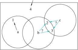
$W$ Var Rng x 1 x 2 y 1 y 2 z 1 z 2 $U_{1}$ D $T_{R}$ Id $a$ 1 $x\mapsto 1$ $b$ 2 $x\mapsto 2$ $b$ 3 $x\mapsto 1$ $c$ 3 $x\mapsto 2$ $c$ 2 $d$ 4 $U_{2}$ D $T_{R}$ Type $a$ Tank $b$ Transport $c$ Tank $y\mapsto 1$ $d$ Tank $y\mapsto 2$ $d$ Transport $U_{3}$ D $T_{R}$ Faction $a$ Friend $b$ Friend $c$ Enemy $z\mapsto 1$ $d$ Friend $z\mapsto 2$ $d$ Enemy

(a)                                                                (b)

Figure 1: Map with moving vehicles (a) and U-relational database representation of the possible worlds at the time the aerial photograph detecting vehicles 1,2,3,4 was taken (b).

U-relations. In this paper, we develop and study U-relations, a representation system that we introduce with the following example.

Example 1.1.

Let us assume that an aerial photograph of a battlefield shows four vehicles at distinct positions 1 to 4. The resolution of the image does not allow for the identification of vehicle types, but we can draw certain conclusions from earlier reconnaissance and a calculation of the maximum distance each vehicle may have covered since. Say we know that vehicle 1 is (a) a friendly tank. Vehicles 2 and 3 are (b) a friendly transport and (c) an enemy tank, but we do not know which one is which. Nothing is known about vehicle 4. Figure 1a shows a schematic drawing of how this scenario can arise. Only 1 is in the range of (a); 2 and 3 are in the ranges of (b) and (c); and position 4 is near the border of the photograph but outside the ranges of (a), (b), and (c), so this vehicle must have newly moved onto the map.

We want to model this by an uncertain database of schema $R$(Id, Coord, Type, Faction), representing the ids (1–4), coordinate positions, types, and factions of the vehicles on the map. Let us assume there are only two vehicle types (tank or transport) and two factions (friend or enemy). Then there are eight possible worlds. We obtain one by taking three choices – answering the following questions: Has the friendly transport (b) now become vehicle 2 ($x\mapsto 1$) or 3 ($x\mapsto 2$)? Is vehicle 4 a tank ($y\mapsto 1$) or a transport ($y\mapsto 2$)? Is vehicle 4 friendly ($z\mapsto 1$) or an enemy ($z\mapsto 2$)? Thus the uncertainty can be naturally modelled using three variables $x,y,z$ that each can independently take one of two values.

We model this scenario by the U-relational database shown in Figure 1b. We use vertical partitioning (cf. e.g. [7, 15]) to achieve attribute-level representation. $R$ is represented using four U-relations, one for each column of $R$. The U-relation for the coordinate positions (which are all certain) is not shown since we do not want to use it subsequently, but of course, conceptually, coordinate positions are an important feature of the example and have to be part of the schema. In addition there is a relation $W$ which defines the possible values the three variables can take.

We can compute a vertical decomposition of one world given by a valuation $\theta$ of the variables $x,y,z$ by (*) removing all the tuples from the U-relations whose $D$ columns contain assignments that are inconsistent with $\theta$ (For example, if $\theta=\{x\mapsto 1,y\mapsto 1,z\mapsto 1\}$ then we remove the third and fifth tuples of $U_{1}$ and the fifth tuples of $U_{2}$ and $U_{3}$.) and then (*) projecting the $D$ columns away. Of course we can resolve the vertical partitioning by joining the decomposed relations on the tuple id columns $T_{R}$. $\Box$

U-relations have the following properties:

• Expressiveness: U-relations are complete for finite sets of possible worlds, that is, they allow for the representation of any finite world-set.

• Succinctness: U-relations represent uncertainty on the attribute level. Even though they allow for more efficient query evaluation, U-relations are, as we show, exponentially more succinct than ULDBs and WSDs. That is, there are (relevant) world-sets that necessarily take exponentially more space to represent by ULDBs or WSDs than by U-relations.

• Leveraging RDBMS technology: U-relations allow for a large class of queries (positive relational algebra extended by the operation “possible”) to be processed using relational algebra only, and thus efficiently in the size of the data. Our approach is the first so far to achieve this for the above-named query language. Indeed, this not only settles that there is a succinct and complete attribute-level representation for which the so-called tuple Q-possibility problem for positive relational algebra is in polynomial time (previously open [6]) but puts a rich body of research results and technology at our disposal for building uncertain database systems.

  This makes U-relations the most efficient and scalable approach to managing uncertain databases to date.

• Parsimonious translation: The translation from relational algebra expressions on the logical schema level to query plans on the physical representations replaces a selection by a selection, a projection by a projection, a join by a join (however, with a more intricate join condition), and a “possible” operation by a projection. We have observed that state-of-the-art RDBMS do well at finding efficient query plans for such physical-level queries.

Ease of use: A main strength of U-relations is their simplicity and low “cost of ownership”:

• The representation system is purely relational and in close analogy with relational representation schemes for vertically decomposed data. Apart from the column store relations that represent the actual data, there is only a single auxiliary relation $W$ (which we need for computing certain answers, but not for possible answers).

• Query evaluation can be fully expressed in relational algebra. The translation is quite simple and can even be done by hand, at least for moderately-sized queries.

• The query plans obtained by our translation scheme are usually handled well by the query optimizers of off-the-shelf relational DBMS, so the implementation of special operators and optimizer extensions is not strictly needed for acceptable performance.

Thus U-relations are not only suited as a representation system for dedicated uncertain database implementations such as MayBMS [4], but are also relevant to “casual users” of representation systems for uncertain data, such as researchers in data cleaning and data integration who want to store and query uncertain data without great effort.

Apart from those implicitly mentioned above, we make the following further contributions in this paper.

• We study algebraic query optimization and present equivalences that hold on vertically decomposed representations. We address query optimization using them in the context of managing uncertainty with U-relations.

• We present an algorithm for normalizing a U-relational representation obtained from a query. Normalized U-relational databases yield a conceptually simple algorithm for computing the certain answers of queries. In particular, certain answer tuples on normalized tuple-level representations can be computed using relational algebra only, which is not true in general for previous representation systems.

• We provide experimental evidence for the efficiency and relevance of our approach.

The structure of the paper is as follows. Section 2 establishes U-relations formally. Section 3 presents our reduction from queries on the logical level to relational algebra on the level of U-relations and addresses algebraic query evaluation. Section 4 presents the normalization algorithm. Section 5 discusses the relationship between U-relations, WSDs and ULDBs and argues that U-relations combine the advantages of the other two formalisms without sharing their drawbacks. In Section 6, we report on our experiments with U-relations. We conclude with Section 7.

2 U-relational databases

We define world-sets in close analogy to the case of c-tables [12]. Consider a finite set of variables over finite domains. A possible world is represented by a total valuation (or assignment) $f:$Var $\mapsto$ Rng of variables to constants in their domains, and the world-set is represented by the finite set of all total valuations. We represent relationally the variable set and the associated domains by a world-table over schema $W$(Var,Rng) such that $W$ consists of all pairs $(x,v)$ of variables $x$ and values $v$ in the domain of $x$.

Example 2.1.

The world-table $W$ in Figure 1 defines three variables $x,y,z$, whose common domain is $\{1,2\}$. The number of worlds defined by $W$ is $2\cdot 2\cdot 2=8$.$\Box$

Given a world-table $W$, a world-set descriptor over $W$, or ws-descriptor for short, is a valuation $\overline{d}$ such that its graph is a subset of $W$. If $\overline{d}$ is a total valuation, then it represents one world. In our examples, to represent the entire world-set we use an empty ws-descriptor, as a shortcut for a singleton ws-descriptor with a new variable with a singleton domain.

We are now ready to define databases of U-relations.

Definition 2.2.

A U-relational database for a world-set over schema $\Sigma=(R_{1}[\overline{A_{1}}],\dots,R_{k}[\overline{A_{k}}])$ is a tuple

$$(U_{1,1},\ldots,U_{1,m_{1}},\ldots,U_{k,1},\ldots,U_{k,m_{k}},W),$$

where $W$ is a world-table and each relation $U_{i,j}$ has schema $U_{i,j}[\overline{D}_{i,j};$ $\overline{T}_{R_{i}};\overline{B_{i,j}}]$ such that $\overline{D}_{i,j}$ defines ws-descriptors over $W$, $\overline{T}_{R_{i}}$ defines tuple ids, and $\overline{B_{i,1}}\cup\dots\cup\overline{B_{i,m_{i}}}=\overline{A}_{i}$.

A ws-descriptor $\{c_{1}\mapsto l_{1},\ldots,c_{k}\mapsto l_{k}\}$ is relationally encoded in $\pi_{\overline{D}_{i,j}}(U_{i,j})$ of arity $n\geq k$ as a tuple $(c_{1}\mapsto l_{1},\ldots,c_{k}\mapsto l_{k},c_{k+1}\mapsto l_{k+1},\ldots,c_{n}\mapsto l_{n})$, where each $c_{i}\mapsto l_{i}$ is a $c_{j}\mapsto l_{j}$ for any $j$ and all $i$ with $1\leq j\leq k<i\leq n$.

Although we speak of vertical partitioning, we do not require the value columns of $U_{i,j}$ to disjointly partition the columns of $R_{i}$. Indeed, overlap may be useful to speed up query evaluation, see e.g. [15].

We next define the semantics of a U-relational database. To obtain a possible world we first choose a total valuation $f$ over $W$. We then process the U-relations tuple by tuple. If the function $f$ extends the ws-descriptor $\overline{d}$ of a tuple of the form $(\overline{d},\overline{t},\overline{a})$ from a U-relation of schema $(\overline{D},\overline{T},\overline{A})$, we insert in that world the values $\overline{a}$ into the $\overline{A}$-fields of the tuple with identifier $\overline{t}$. In general this may leave some tuples partial in the end (i.e., the values for some fields have not been provided.) These tuples are removed from the world.

We require, for a U-relational database $(U_{1},\ldots,U_{n},W)$ to be considered valid, that the representation does not provide several contradictory values for a tuple field in the same world. Formally, we require, for all $1\leq i,j\leq n$, and tuples $t_{1}\in U_{i}[\overline{D}_{i},\overline{T}_{i},\overline{A}_{i}]$ and $t_{2}\in U_{j}[\overline{D}_{j},\overline{T}_{j},\overline{A}_{j}]$ such that $U_{i}$ and $U_{j}$ are vertical partitions of the same relation, that if there is a world that extends both $t_{1}.\overline{D}_{i}$ and $t_{2}.\overline{D}_{j}$, then for all $A\in(\overline{A}_{i}\cap\overline{A}_{j})$, $t_{1}.A=t_{2}.A$ must hold.

Example 2.3.

Suppose there are two U-relations with schemata $U_{1}[\overline{D_{1}};T_{R};A,B]$ and $U_{2}[\overline{D_{2}};T_{R};B,C]$ that jointly represent columns $A$, $B$, and $C$ of a relation $R$. Assume tuples $(c_{1},1,t_{1},a,b)\in U_{1}$ and $(c_{2},2,t_{1},b^{\prime},c)\in U_{2}$. Then $U_{1}$ and $U_{2}$ cannot form part of a valid U-relational database because there would be a world with $c_{1}\mapsto 1,c_{2}\mapsto 2$ in which the tuple from $U_{1}$ requires field $t_{1}.B$ to take value $b$ while the tuple from $U_{2}$ requires the same field to take value $b$’.$\Box$

A salient property of U-relational databases is that they form a complete representation system for finite world-sets.

Theorem 2.4.

Any finite set of worlds can be represented as a U-relational database.

3 Query Processing

The semantics of a query $Q$ on a world-set is to evaluate $Q$ in each world. For complete representation systems like U-relational databases, there is an equivalent, more efficient approach [12]: Translate $Q$ into a query $\hat{Q}$ such that the evaluation of $\hat{Q}$ on a U-relational encoding of the world-set produces the U-relational encoding of the answer to $Q$.

Queries on vertical decompositions. U-relations rely essentially on vertical decomposition for succinct (attribute-level) representation of uncertainty. To evaluate a query, we first need to reconstruct relations from vertical decompositions by (1) joining two partitions on the common tuple id attributes and (2) discarding the combinations that yield inconsistent ws-descriptors. We call this operation merge and give its precise definition in Figure 4, where the two above conditions are defined by $\alpha$ and $\psi$, respectively.

Example 3.1.

Consider the U-relational database of Figure 1. The query $\sigma_{\mathrm{Faction=^{\prime}Enemy^{\prime}}\wedge\mathrm{Type=^{\prime}Tank^{\prime}}}(R)$ lists the enemy tanks on the map. To answer this query, we need to merge the necessary partitions of $R$ and obtain a new query with $merge(\pi_{\mathrm{Faction}}(R),\pi_{\mathrm{Type}}(R))$ in the place of $R$. $\Box$

Our query evaluation approach can take full advantage of query evaluation and optimization techniques on vertical partitions. First, it does not require to reconstruct the entire relations involved in the query, but rather only the necessary vertical partitions. Second, necessary partitions can be flexibly merged in during query evaluation. Thus early and late tuple materialization [15] carry over naturally to our framework. For this, our merge operator allows to merge two partitions not only if they are given in their original form, but also if they have been modified by queries.

The first advantage only holds for so-called reduced U-relational databases, which do not have tuples that cannot be completed in any world. That is, each tuple of a reduced U-relation can always be completed to an actual tuple in a world. The advantage becomes evident even for a simple projection query. Consider a reduced database containing a U-relation $U$ defining the $A$ attribute of $R$. To evaluate $\pi_{A}(R)$ we do not need to merge in all U-relations defining the attributes of $R$ and later project on $A$. Instead, the answer is simply $U$. In the following, we assume that the input database is always reduced. As we will discuss next, our query evaluation technique always produces reduced U-relations for reduced input U-relational databases.

Example 3.2.

Consider the following non-reduced database of two U-relations:

$U_{1}$ $D$ $T$ A $c_{1}\mapsto 1$ $t_{1}$ $a_{1}$ $c_{2}\mapsto 1$ $t_{2}$ $a_{2}$     $U_{2}$ $D$ $T$ B $c_{1}\mapsto 1$ $t_{1}$ $b_{1}$ $c_{1}\mapsto 2$ $t_{1}$ $b_{2}$

In each U-relation the second tuple cannot find a partner in the other U-relation with which a complete tuple (with both attributes A and B) can be formed. If these second tuples are removed, the database is reduced. $\Box$

We can always reduce a U-relational database as follows: We filter each U-relation using semijoins with each of the other U-relations representing data of the same relation $R_{i}$. The semijoin conditions are the $\alpha$ and $\psi$-conditions.

Proposition 3.3.

Given a schema $\Sigma$, there is a relational algebra query that reduces a U-relational database over $\Sigma$.

$$merge(\pi_{\overline{X}}(R),\pi_{\overline{A}-\overline{X}}(R))=R,\hskip 20.00003pt\mbox{ where }\overline{A}=\textbf{sch}(R)$$ (1)

$$merge(R,S)=merge(S,R)$$ (2)

$$merge(merge(R,S),T)=merge(R,merge(S,T))$$ (3)

$$\sigma_{\phi(\overline{X})}(merge(R,S))=merge(\sigma_{\phi(\overline{X})}(R),S)$$ (4)

$$\hskip 80.00012pt\mbox{ where }\overline{X}\subseteq\textbf{sch}(R)$$

$$merge(R,S)\bowtie_{\phi(\overline{X},\overline{Y})}T=merge(R\bowtie_{\phi(\overline{X},\overline{Y})}T,S)$$ (5)

$$\hskip 80.00012pt\mbox{ where }\overline{X}\cup\overline{Y}\subseteq\textbf{sch}(R)\cup\textbf{sch}(T)$$

$$\pi_{\overline{X}}(merge(R,S))=merge(\pi_{\overline{X}\cap\overline{A}}(R),\pi_{\overline{X}\cap\overline{B}}(S))$$ (6)

$$\hskip 80.00012pt\mbox{ where }\textbf{sch}(R)=\overline{A},\textbf{sch}(S)=\overline{B}$$

Figure 2: Algebraic equivalences for relational algebra queries with merge operator.

Algebraic equivalences. Figure 2 gives algebraic equivalences of relational algebra expressions with merge operator on vertical decompositions: Merging is the reverse of vertical partitioning, it is commutative and associative, it commutes with selections, joins, and projections.

Standard heuristics known from classical query optimization for relational algebra apply here as well. Intuitively, we usually push down projections and selections and merge in U-relations as late as possible. An interesting new case is the decision on join ordering among an explicit join from the input query and a join due to merging: If the merge is executed before the explicit join, it may reduce the size of an input relation to join. We have seen in our experiments that the standard selectivity-based cost measures employed by relational database management systems do a good job, as long as the queries remain reasonably small.

[levelsep=.7cm,treesep=.4cm,nodesep=.05cm]$\pi_{\textrm{DATE}}$ $\bowtie_{\textrm{CUSTKEY}}$ $\sigma_{\textrm{NAME=Al}}$ Cust $\sigma_{\textrm{DATE$>$2003}}$ merge $\pi_{\textrm{DATE}}(\textrm{Ord})$ $\pi_{\textrm{CUST}}(\textrm{Ord})$

Query plan P1.

[levelsep=.7cm,treesep=.4cm,nodesep=.05cm]$\pi_{\textrm{DATE}}$ $\bowtie_{\textrm{CUSTKEY}}$ $\sigma_{\textrm{NAME=Al}}$ Cust merge $\sigma_{\textrm{DATE$>$2003}}$ $\pi_{\textrm{DATE}}(\textrm{Ord})$ $\pi_{\textrm{CUST}}(\textrm{Ord})$	[levelsep=.7cm,treesep=.4cm,nodesep=.05cm]merge $\pi_{\emptyset}$ $\bowtie_{\textrm{CUSTKEY}}$ $\sigma_{\textrm{NAME=Al}}$ Cust $\pi_{\textrm{CUST}}(\textrm{Ord})$ $\sigma_{\textrm{DATE$>$2003}}$ $\pi_{\textrm{DATE}}(\textrm{Ord})$
Query plan P2.	Query plan P3.

Figure 3: Three equivalent query plans.

Example 3.4.

Consider a U-relational database ${\cal U}$ that represents a set of possible worlds over two TPC-H relations Ord and Cust (short for Order and Customer, respectively) [16]. ${\cal U}$ has one U-relation for each attribute of the two relations, of which we only list DATE and CUSTKEY for Ord, and NAME and CUSTKEY for Cust. The following query finds all dates of orders placed by Al after 2003:

$$\pi_{\mathrm{DATE}}( \sigma_{\mathrm{NAME=^{\prime}Al^{\prime}}}(\mathrm{Cust})\bowtie_{\mathrm{CUSTKEY}}\sigma_{\mathrm{DATE>2003}}(\mathrm{Ord}))$$

Figure 3 shows three possible plans P1, P2, and P3 using operators on vertical decompositions. The naïve plan P1 first reconstructs Ord from its two partitions then applies the selection and the join with Cust. In P2 and P3 the merge operator is pushed up in the plans, first immediately above the selection (P2), and then above the join operator (P3). Among the three plans, P1 is clearly the least efficient. However, without statistics about the data, one cannot tell which of P2 and P3 should be preferred. If DATE$>$2003 is very selective, then merging immediately thereafter as in P2 will lead to filtering of tuples from $\pi_{\mathrm{CUSTKEY}}(\mathrm{Ord})$ and thus fewer tuples will be processed by the join. Is this not the case, then first merging only increases the number and size of the tuples that have to be processed by the join. Also, in P3 all value attributes except of DATE are projected away after the join as they are not needed for the final result. $\Box$

Queries on U-relations. Figure 4 gives the function $[\![\cdot]\!]$ that translates positive relational algebra queries with poss and merge operators into relational algebra queries on U-relational databases.

The poss operator applied on a U-relation $U$ closes the possible worlds semantics by computing the set of tuples possible in $U$. It thus translates to a simple projection on the value attributes of $U$. The result of a projection is a U-relation whose value attributes are those from the projection list (thus the input ws-descriptors and tuple ids are preserved). Selections apply conditions on the value attributes.

The merge operator that reconstructs a relation from its vertical partitions was already explained. Similarly to the merge, the join uses the $\psi$-condition to discard tuple combinations with inconsistent ws-descriptors. Figure 4 gives the translation in case $U_{1}$ and $U_{2}$ do not contain partitions of the same relation. For the case of self-joins we require aliases for the copies of the relation involved in it such that they do not have common tuple id attributes.

The union of $U_{1}$ and $U_{2}$ like the ones from Figure 4 is sketched next. We assume that $\overline{A}_{1}=\overline{A}_{2}$, $\overline{T}_{1}\cap\overline{T}_{2}=\emptyset$, and the tuples of different relations have different ids. To bring $U_{1}$ and $U_{2}$ to the same schema, we first ensure ws-descriptors of the same size by pumping in the smaller ws-descriptors already contained variable assignments, and add new (empty) columns $\overline{T}_{2}$ to $U_{1}$ and $\overline{T}_{1}$ to $U_{2}$. We then perform the standard union.

$\displaystyle\mbox{Let }U_{1}$ $\displaystyle:=[\![Q_{1}]\!]\mbox{ with schema }[\overline{D}_{1},\overline{T}_{1},\overline{A}_{1}],\hskip 30.00005pt$ $\displaystyle U_{2}$ $\displaystyle:=[\![Q_{2}]\!]\mbox{ with schema }[\overline{D}_{2},\overline{T}_{2},\overline{A}_{2}],$ $\displaystyle\alpha$ $\displaystyle:=\underset{T\in\overline{T}_{1}\cap\overline{T}_{2}}{\bigwedge}(U_{1}.T=U_{2}.T),$ $\displaystyle\psi$ $\displaystyle:=\underset{D^{\prime}\in U_{1}.\overline{D}_{1},D^{\prime\prime}\in U_{2}.\overline{D}_{2}}{\bigwedge(D^{\prime}.\mbox{Var}=D^{\prime\prime}}.\mbox{Var}\Rightarrow D^{\prime}.\mbox{Rng}=D^{\prime\prime}.\mbox{Rng}).$ $\displaystyle[\![poss(Q_{1})]\!]$ $\displaystyle:=\pi_{\overline{A}_{1}}(U_{1})$ $\displaystyle[\![\pi_{\overline{X}}(Q_{1})]\!]$ $\displaystyle:=\pi_{\overline{D}_{1},\overline{T}_{1},\overline{X}}(U_{1}),\hskip 10.00002pt\mbox{where }\overline{X}\subseteq\overline{A}_{1}$ $\displaystyle[\![\sigma_{\phi}(Q_{1})]\!]$ $\displaystyle:=\sigma_{\phi}(U_{1}),\hskip 30.00005pt\mbox{where }\phi\mbox{ on }\overline{A}_{1}$ $\displaystyle[\![Q_{1}\bowtie_{\phi}Q_{2}]\!]$ $\displaystyle:=\pi_{\overline{D}_{1},\overline{D}_{2},\overline{T}_{1},\overline{T}_{2},\overline{A},\overline{B}}(U_{1}\bowtie_{\phi\land\psi}U_{2}),\hskip 30.00005pt$ $\displaystyle\hskip 75.0001pt\mbox{ where }\overline{T}_{1}\cap\overline{T}_{2}=\emptyset$ $\displaystyle[\![merge(Q_{1},Q_{2})]\!]$ $\displaystyle:=\pi_{\overline{D}_{1},\overline{D}_{2},\overline{T}_{1}\cup\overline{T}_{2},\overline{A},\overline{B}}(U_{1}\bowtie_{\alpha\land\psi}U_{2})$

Figure 4: Translation of queries with merge into queries on U-relations.

From our translation $[\![\cdot]\!]$ it immediately follows that

Theorem 3.5.

Positive relational algebra queries extended with the possible operator can be evaluated on U-relational databases using relational algebra only.

Example 3.6.

Recall the U-relational database of Figure 1 storing information about moving vehicles. Consider a query asking for ids of enemy tanks:

$$S=\pi_{\mathrm{Id}}(\sigma_{\mathrm{Type=^{\prime}Tank^{\prime}}\wedge\mathrm{Faction=^{\prime}Enemy^{\prime}}}(\mathit{R}))$$

After merging the necessary partitions of relation $R$ and translating it into positive relational algebra, we obtain

$$\pi_{\mathrm{Id}}(\sigma_{\mathrm{Type=^{\prime}Tank^{\prime}}\wedge\mathrm{Faction=^{\prime}Enemy^{\prime}}}(U_{1}\bowtie_{\alpha_{1}\land\psi_{1}}U_{2}\bowtie_{\alpha_{2}\land\psi_{2}}U_{3})),$$

where the conditions $\psi_{1}$, $\psi_{2}$, $\alpha_{1}$, and $\alpha_{2}$ follow the translation given in Figure 4. The three vertical partitions are joined on the tuple id attributes ($\alpha_{1}$ and $\alpha_{2}$) and the combinations with conflicting mappings in the ws-descriptors are discarded ($\psi_{1}$ and $\psi_{2}$). Before and after translation, the query is subject to optimizations as discussed earlier. (In this case, a good query plan would first apply the selections on the partitions, then project away the irrelevant value attributes Type and Faction, and then merge the partitions).

$U_{4}$ $D_{1}$ $D_{2}$ T_S Id $x\mapsto 1$ $c$ 3 $x\mapsto 2$ $c$ 2 $y\mapsto 1$ $z\mapsto 2$ $d$ 4

The above U-relation $U_{4}$ encodes the query answer.$\Box$

Example 3.7.

We continue Example 3.6 and ask whether it is possible that the enemy has two tanks on the map, and if so, which vehicles are those. For this, we compute the pairs of enemy tanks as a self-join of $S$: $(S\ s_{1})\bowtie_{s_{1}.\mathrm{Id}\not=s_{2}.\mathrm{Id}}(S\ s_{2})$. This query is in turn equivalent to a self-join of $U_{4}$.

$U_{5}$ $D_{1}$ $D_{2}$ $D_{3}$ T${}_{s_{1}}$ T${}_{s_{2}}$ Id₁ Id₂ $x\mapsto 1$ $y\mapsto 1$ $z\mapsto 2$ $c$ $d$ 3 4 $x\mapsto 2$ $y\mapsto 1$ $z\mapsto 2$ $c$ $d$ 2 4 $y\mapsto 1$ $z\mapsto 2$ $x\mapsto 1$ $d$ $c$ 4 3 $y\mapsto 1$ $z\mapsto 2$ $x\mapsto 2$ $d$ $c$ 4 2

The answer is encoded by the above U-relation $U_{5}$. Note that the combinations of the first two tuples of $U_{4}$ are not in $U_{5}$, because they have inconsistent ws-descriptors and are filtered out using the $\psi$-condition (vehicle $c$ cannot be at the same time at two different positions). To obtain the possible pairs of vehicle ids, we apply the poss operator on $U_{5}$. This is expressed as the projection on the value attributes of $U_{5}$.$\Box$

Our translation yields relational algebra queries, whose evaluation always produces tuple-level U-relations, i.e., U-relations without vertical decompositions, by joining and merging vertical partitions of relations. Following the definition of the merge operator, if the input U-relations are reduced, then the result of merging vertical partitions is also reduced. We thus have that

Proposition 3.8.

Given a positive relational algebra query $Q$ and a reduced U-relational database $U$, $[\![Q]\!](U)$ is a reduced U-relational database.

4 Normalization of U-relations

Input: Reduced U-relational database ${\cal U}=(U_{1},\dots,U_{m},W)$

Output: Normalized reduced U-relational database.

begin  $R$ := the relation consisting of all pairs of variables $(c_{i},c_{j})$ that occur together in some ws-descriptor of ${\cal U}$;

${\cal G}$ := the graph whose node set is the set of variables and whose edge relation is the refl. and trans. closure of $R$;

Compute the connected components of ${\cal G}$;

foreach U-relation $U_{j}(D_{1},\ldots,D_{n},\overline{T},\overline{A})$ of ${\cal U}$ do  $U^{\prime}_{j}$ := empty U-relation over $U^{\prime}_{j}(\mbox{Var},\mbox{Rng},\overline{T},\overline{A})$;

foreach $t\in U$ do  $G_{i}$ := connected component of ${\cal G}$ with id $i$ such that the nodes $t.\mbox{Var}_{1},\ldots,t.\mbox{Var}_{n}$ are in $G_{i}$;

$\{c_{i_{1}},\ldots,c_{i_{k}}\}=G_{i}-\{t.\mbox{Var}_{1},\ldots,t.\mbox{Var}_{n}\}$;

foreach $l_{i_{1}}:(c_{i_{1}},l_{i_{1}})\in W,\ldots,l_{i_{k}}:(c_{i_{k}},l_{i_{k}})\in W$ do  /* Compute a new domain value ($f_{|G_{i}|}$ is either the identity or better, for atomic $l$’s, an injective function $\mbox{int}^{|G_{i}|}\rightarrow\mbox{int}$) */;

$l$ := $f_{|G_{i}|}(t.\overline{\mbox{Rng}},l_{i_{1}},\ldots,l_{i_{k}})$;

$U_{j}^{\prime}:=U_{j}^{\prime}\cup\{(G_{i},l,t.\overline{T},t.\overline{A})\}$;

      $W^{\prime}:=\bigcup_{i}\{(g_{i},(l_{1},\dots,l_{m}))\mid G_{i}=\{c_{1},\dots,c_{m}\}\mbox{ and}$

                                 $\;(c_{1},l_{1}),\dots,(c_{m},l_{m})\in W\}$;

Output $(U_{1}^{\prime},\dots,U_{m}^{\prime},W^{\prime})$;

end

Algorithm 1 Normalization of ws-descriptors.

U-relations do not forbid large ws-descriptors. The ability to extend the size of ws-descriptors is what yields efficient query evaluation on U-relations. However, large ws-descriptors cause an inherent processing overhead. Also, after query evaluation or dependency chasing on a U-relational database, it may happen that tuple fields, which used to be dependent on each other, become independent. In such a case, it is desirable to optimize the world-set representation [6]. We next discuss one approach to normalize U-relational databases by reducing large ws-descriptors to ws-descriptors of size one. Normalization is an expensive operation per se, but it is not unrealistic to assume that uncertain data is initially in normal form [4, 6] and can subsequently be maintained in this form.

Definition 4.1.

A U-relational database is normalized if all ws-descriptors of its U-relations have size one.

Algorithm 1 gives a normalization procedure for U-relations that determines classes of variables that co-occur in some ws-descriptors and replaces each such class by one variable, whose domain becomes the product of the domains of the variables from that class. Figure 5 shows a U-relational database and its normalization.

Theorem 4.2.

Given a reduced U-relational database, Algorithm 1 computes a normalized reduced U-relational database that represents the same world-set.

$U$ $D_{1}$ $D_{2}$ $T$ $A$ $c_{1}\mapsto 1$ $c_{1}\mapsto 1$ $t_{1}$ $a_{1}$ $c_{1}\mapsto 1$ $c_{2}\mapsto 2$ $t_{2}$ $a_{2}$ $c_{1}\mapsto 2$ $c_{1}\mapsto 2$ $t_{2}$ $a_{3}$ $c_{3}\mapsto 1$ $c_{3}\mapsto 1$ $t_{3}$ $a_{4}$ $c_{3}\mapsto 2$ $c_{3}\mapsto 2$ $t_{3}$ $a_{5}$

$W$ Var Rng $c_{1}$ 1 $c_{1}$ 2 $c_{2}$ 1 $c_{2}$ 2 $c_{3}$ 1 $c_{3}$ 2

(a) U-relational database

$U^{\prime}$ $D$ $T$ $A$ $c_{12}\mapsto(1,1)$ $t_{1}$ $a_{1}$ $c_{12}\mapsto(1,2)$ $t_{1}$ $a_{1}$ $c_{12}\mapsto(1,2)$ $t_{2}$ $a_{2}$ $c_{12}\mapsto(2,1)$ $t_{2}$ $a_{3}$ $c_{12}\mapsto(2,2)$ $t_{2}$ $a_{3}$ $c_{3}\mapsto 1$ $t_{3}$ $a_{4}$ $c_{3}\mapsto 2$ $t_{3}$ $a_{5}$

$W^{\prime}$ Var Rng $c_{12}$ $(1,1)$ $c_{12}$ $(1,2)$ $c_{12}$ $(2,1)$ $c_{12}$ $(2,2)$ $c_{3}$ $1$ $c_{3}$ $2$

(b) Database from (a) normalized

$c_{12}$ $t_{1}.A$ $t_{2}.A$ $(1,1)$ $a_{1}$ $\bot$ $(1,2)$ $a_{1}$ $a_{2}$ $(2,1)$ $\bot$ $a_{3}$ $(2,2)$ $\bot$ $a_{3}$ $\times$ $c_{3}$ $t_{3}.A$ 1 $a_{4}$ 2 $a_{5}$

(c) WSD corresponding to (b)

Figure 5: Normalization example.

Computing certain answers. Given a set of possible worlds, we call a tuple certain iff it occurs in each of the worlds. It is known that the tuple certainty problem is coNP-hard for a number of representation systems, ranging from attribute-level ones like WSDs to tuple-level ones like ULDBs [6]. In case of tuple-level normalized U-relations, however, we can efficiently compute the certain tuples using relational algebra.

Lemma 4.3.

A tuple $\overline{t}$ is certain in a tuple-level normalized U-relation $U$ iff there exists a variable $x$ such that $(x\mapsto l,\overline{s},\overline{t})\in U$ for each domain value $l$ of $x$ and some tuple id $\overline{s}$.

The condition of the lemma can be encoded as the following domain calculus expression:

$$cert(U):=\{\overline{t}\ |\ \exists x\forall l\;(x,l)\in W\Rightarrow\exists\overline{s}(x,l,\overline{s},\overline{t})\in U\}$$

The equivalent relational algebra query on a tuple-level normalized U-relational database $(U[\mbox{Var},\mbox{Rng},\overline{T_{R}},\overline{A}],W)$ is

$$\pi_{\overline{A}}(\pi_{\mathit{Var}}(W)\times\pi_{\overline{A}}(U)-\pi_{\mathit{Var},\overline{A}}(W\times\pi_{\overline{A}}(U)-\pi_{\mathit{Var},\mathit{Rng},\overline{A}}U)).$$

5 Succinctness and Efficiency

This section compares U-relational databases with WSDs [4, 6] and ULDBs [8] using two yardsticks: succinctness, i.e., how compactly can they represent world-sets, and efficiency of query evaluation.

WSDs vs. U-Relations. WSDs are essentially normalized U-relational databases where each variable $c_{i}$ of a U-relation corresponds to a WSD component relation $C_{i}$ and each domain value $l_{i}$ of $c_{i}$ corresponds to a tuple of $C_{i}$. Figure 5(c) shows a WSD equivalent to a normalized U-relational database. The normalization may lead to an exponential blow-up in the database size and accounts for U-relations with arbitrarily large ws-descriptors being more compact than U-relations with singleton ws-descriptors and thus than WSDs.

$c_{1}$ $t_{1}.A$ $t_{2}.B$ $w_{1}$ $1$ $1$ $w_{2}$ $0$ $0$ $\times\cdots\times$ $c_{n}$ $t_{n}.A$ $t_{1}.B$ $w_{1}$ $1$ $1$ $w_{2}$ $0$ $0$

(a) WSD encoding.

$U_{1}$ $D$ $T$ $A$ $c_{1}\mapsto w_{1}$ $t_{1}$ $1$ $c_{1}\mapsto w_{2}$ $t_{1}$ $0$ $\vdots$ $c_{n}\mapsto w_{1}$ $t_{n}$ $1$ $c_{n}\mapsto w_{2}$ $t_{n}$ $0$     $U_{2}$ $D$ $T$ $B$ $c_{2}\mapsto w_{1}$ $t_{2}$ $1$ $c_{2}\mapsto w_{2}$ $t_{2}$ $0$ $\vdots$ $c_{n}\mapsto w_{1}$ $t_{1}$ $1$ $c_{n}\mapsto w_{2}$ $t_{1}$ $0$

(b) U-relational encoding.

Figure 6: WSD and U-relational encoding of the world-set of Example 5.1.

Example 5.1.

Consider a relation over schema $R[AB]$ where each field value can be 0 or 1, and $t_{i}.A$ and the tuple fields $t_{(i+1)\mbox{ mod }n}.B$ depend on each other ($1\leq i\leq n$). The encodings as WSD and as a set of two U-relations are given in Figure 6.$\Box$

Theorem 5.2.

U-relational databases are exponentially more succinct than WSDs.

Positive relational queries have polynomial data complexity for U-relations (Section 3) and exponential data complexity for WSDs [6]. This can be explained in close analogy to the difference in succinctness and by the fact that query evaluation creates new dependencies [10]: U-relations can efficiently store the new dependencies by enlarging ws-descriptors, whereas WSDs correspond to U-relations with normalized ws-descriptors, hence the exponential blowup.

$c_{1}\times\cdots\times c_{n}$ $t_{1}.A$ $t_{2}.B$ $\ldots$ $t_{n}.A$ $t_{1}.B$ $w_{1}$ $1$ $1$ $\ldots$ $1$ $1$ $w_{2}$ $0$ $0$ $\ldots$ $0$ $0$ $w_{3}$ $\bot$ $1$ $\ldots$ $1$ $\bot$ $\vdots$ $w_{2^{n}}$ $\bot$ $\bot$ $\ldots$ $\bot$ $\bot$

(a) WSD encoding.

$U_{3}$ $D_{1}$ $D_{2}$ $T$ $A$ $B$ $c_{2}\mapsto w_{1}$ $c_{3}\mapsto w_{1}$ $t_{2}$ $1$ $1$ $c_{2}\mapsto w_{2}$ $c_{3}\mapsto w_{2}$ $t_{2}$ $0$ $0$ $\vdots$ $c_{1}\mapsto w_{1}$ $c_{n}\mapsto w_{1}$ $t_{1}$ $1$ $1$ $c_{1}\mapsto w_{2}$ $c_{n}\mapsto w_{2}$ $t_{1}$ $0$ $0$

(b) U-relational encoding.

Figure 7: WSD and U-relation representing the answer to $\sigma_{A=B}(R)$ with $R$ of Figure 6.

Example 5.3.

Consider the WSD and U-relations of Example 5.1 and the selection with join condition $\sigma_{A=B}(R)$. The answer is represented by the WSD and U-relation respectively shown in Figure 7. The U-relation $U_{3}$ has $2\cdot n$ tuples, whereas the WSD $c_{1}\times\cdots\times c_{n}$ has $2^{n}$ tuples, each representing a possible combination of the values of the existing fields (a tuple $t_{i}$ does not occur in worlds where $t_{i}.A$ or $t_{i}.B$ have values $\bot$). Note that by normalizing $U_{3}$ we would also obtain one variable with $2^{n}$ domain values, as for the WSD.

The answer to $\mathit{poss}(\sigma_{A=B}(R))$ is efficiently computed as $\pi_{A,B}(U_{3})$ in the case of U-relations. In the WSD case, it is computed as $\underset{i}{\overset{n}{\cup}}(\pi_{t_{i}.A,t_{i}.B}(c_{1}\times\cdots\times c_{n}))$. $\Box$

Finally, the query translations employed by the evaluation algorithms in the WSD and U-relational cases are different. Whereas for WSDs all operators are translated to sequences of relational queries and in the case of projection and join even to fixpoint programs [4], the translation remains strictly in relational algebra for U-relations.

ULDBs vs. U-Relations. A ULDB relation is a set of x-tuples, where each x-tuple represents a set of alternatives. One world is defined by choosing precisely one alternative of each x-tuple. A world may contain none of the alternatives of an x-tuple, if this x-tuple is marked as optional (or maybe) using the ?-symbol. Dependencies between alternatives of different x-tuples are enforced using lineage: An alternative $i$ of an x-tuple $s$ occurs in the same worlds with an alternative $j$ of another x-tuple $t$ if the lineage of $(s,i)$ points either to $(t,j)$, or to another alternative that transitively points to $(t,j)$. The lineage of an alternative can also point to an external symbol $(t,j)$, if there is no alternative $(t,j)$ in the database [8].

Example 5.4.

The U-relations representing relation $R$ in Figure 1 admit the following equivalent ULDB:

      R (Id, Type, Faction) $a$ 1: (1, Tank, Friend) $b$ 1: (2, Transport, Friend) $||$ 2: (3, Transport, Friend) $\Lambda$ $c$ 1: (3, Tank, Enemy) $||$ 2: (2, Tank, Enemy) $d$ 1: (4, Tank, Friend) $||$ 2: (4, Tank, Enemy) $||$ 3: (4, Transport, Friend) $||$ 4: (4, Transport, Enemy)

$$\Lambda\mbox{ is } \lambda(b,1)=\{(c,1)\},\lambda(b,2)=\{(c,2)\}$$

To construct an ULDB equivalent to the U-relational database of Figure 1, we have to enumerate all possible value combinations for the attributes of $R$. This enumeration is not necessary for U-relations because of vertical partitioning and the independence of (most) tuple fields. $\Box$

Lemma 5.5.

ULDBs [8] can be translated linearly into U-relational databases.

Proof.

We sketch the proof for a single ULDB relation $R$; it can be extended trivially to the case of several relations.

For every x-tuple $t$ in $R$ we create a new variable $c_{t}$, and for each alternative $j$ of $t$ we create a new domain value $w_{(t,j)}$ of $c_{t}$. For every alternative in $R$ with value $a$, id $(t,j)$ and lineage $\lambda(t,j)=\overset{n_{(t,j)}}{\underset{i}{\bigwedge}}(t_{i},j_{i})$ we create a tuple in $U^{R}$ with value $a$, tuple id $t$ and ws-descriptor ($n=n_{(t,j)}$)

$$D_{(t,j)}=[(c_{t},w_{(t,j)}),(c_{t_{1}},w_{(t_{1},j_{1})}),\ldots,(c_{t_{n}},w_{(t_{n},j_{n})})].$$

In case $n_{(t,j)}$ is smaller than $n_{(s,l)}$ of an alternative $l$ of an x-tuple $s$, then we pad the above ws-descriptor with $n_{(s,l)}-n_{(t,j)}$ pairs $(c_{t},w_{(t,j)})$.

The world table $W$ is the set of pairs of variables and domain values created for the x-tuples of $R$. For each optional x-tuple $t$ in $R$, we also add to $W$ a tuple $(c_{t},w)$ where $w$ is a fresh domain value for $c_{t}$. ∎

There are U-relations, however, whose ULDB encodings are necessarily exponential in the arity of the logical relation. This is the case of, e.g., or-set relations [13], attribute-level representations that can be linearly encoded as U-relations but exponentially as ULDBs.

Theorem 5.6.

U-relational databases are exponentially more succinct than ULDBs.

Both ULDBs and U-relations have polynomial data complexity for positive relational queries. Differently from ULDBs, evaluating queries on U-relations is possible using relational algebra only. The main difference between their evaluation algorithms concerns erroneous tuples, i.e., tuples that do not appear in any world. In contrast to U-relations, erroneous tuples may appear in the answers to queries on ULDBs (see [8] for an example). The removal of such tuples is called data minimization, an expensive operation that involves the computation of the transitive closure of lineage [8]. Such tuples occur with ULDBs because the lineage of an alternative in the answer only points to the lineage of alternatives from the input relations, even though these input alternatives may not occur in the same world. This cannot happen with U-relations because each query operation ensures that only valid tuples are in the query answer by (1) using the $\psi$-condition in the join and merge operations and by (2) carrying all dependencies in the ws-descriptors – and not only to tuples of the input relation.

To sum up, U-relations have the advantages of WSDs (attribute-level representation) and ULDBs (polynomial evaluation of positive relational algebra queries), while forming an exponentially more succinct representation system than both aforementioned approaches.

$Q_{1}$: possible (select o.orderkey, o.orderdate, o.shippriority from customer c, orders o, lineitem l where c.mktsegment $=$ ’BUILDING’
and c.custkey $=$ o.custkey and o.orderkey $=$ l.orderkey
and o.orderdate $>$ ’1995-03-15’ and l.shipdate $<$ ’1995-03-17’)
$Q_{2}$: possible (select extendedprice from lineitem where
shipdate between ’1994-01-01’ and ’1996-01-01’
and discount between ’0.05’ and ’0.08’ and quantity $<$ 24)
$Q_{3}$: possible (select n1.name, n2.name from supplier s, lineitem l,
orders o, customer c, nation n1, nation n2 where n2.nation=’IRAQ’
and n1.nation=’GERMANY’ and c.nationkey $=$ n2.nationkey
and s.suppkey $=$ l.suppkey and o.orderkey $=$ l.orderkey
and c.custkey $=$ o.custkey and s.nationkey $=$ n1.nationkey)

Figure 8: Queries used in the experiments.

scale	correlation	TPC-H dbsize	#worlds	lworlds	dbsize	#worlds	lworlds	dbsize	#worlds	lworlds	dbsize
0.01	0.10	17	$10^{857.076}$	21	82	$10^{7955.30}$	57	85	$10^{79354.1}$	57	114
0.01	0.25	17	$10^{729.529}$	33	82	$10^{6728.24}$	129	85	$10^{66995.5}$	193	118
0.01	0.50	17	$10^{523.031}$	71	82	$10^{4724.56}$	901	88	$10^{46675.6}$	662	139
0.05	0.10	85	$10^{4287.23}$	22	389	$10^{39913.8}$	33	403	$10^{396137}$	65	547
0.05	0.25	85	$10^{3633.49}$	57	389	$10^{33702.3}$	148	405	$10^{334450}$	158	567
0.05	0.50	85	$10^{2549.14}$	178	390	$10^{23515.5}$	449	416	$10^{232650}$	1155	672
0.10	0.10	170	$10^{8606.77}$	27	773	$10^{79889.9}$	49	802	$10^{793611}$	53	1090
0.10	0.25	170	$10^{7276.46}$	74	774	$10^{67477.1}$	145	806	$10^{670090}$	172	1132
0.10	0.50	170	$10^{5044.65}$	181	776	$10^{46901.8}$	773	826	$10^{466038}$	924	1339
0.50	0.10	853	$10^{43368.0}$	49	3843	$10^{400185}$	71	3987	$10^{3.96845e+06}$	85	5427
0.50	0.25	853	$10^{36630.3}$	130	3845	$10^{337905}$	172	4008	$10^{3.35095e+06}$	320	5632
0.50	0.50	853	$10^{25528.9}$	214	3856	$10^{234840}$	1832	4012	$10^{2.33083e+06}$	2586	6682
1.00	0.10	1706	$10^{87203.0}$	57	7683	$10^{800997}$	99	7971	$10^{7.93774e+06}$	113	11264
1.00	0.25	1706	$10^{73652.5}$	170	7687	$10^{676223}$	208	8012	$10^{6.70229e+06}$	344	11280
1.00	0.50	1706	$10^{51290.9}$	993	7712	$10^{470401}$	1675	8228	$10^{4.66222e+06}$	3392	13312
		$\mathbf{x}=0.0$	$\mathbf{x}=0.001$			$\mathbf{x}=0.01$			$\mathbf{x}=0.1$

Figure 9: Total number of worlds, max. number of local worlds in a component, and size in MB of the U-relational database for each of our settings.

6 Experiments

Prototype Implementation. We implemented the query translator of Figure 4 and also extended the C implementation of the TPC-H population generator version 2.6 build 1 [16] to generate attribute and tuple-level U-relations and ULDBs. The code is available on the MayBMS project page (http://www.infosys.uni-sb.de/projects/maybms).

Setup. The experiments were performed on a 3GHZ/1GB Pentium running Linux 2.6.13 and PostgreSQL 8.2.3.

Generation of uncertain data. Our data generator creates eight tables: part, partsupp, supplier, customer, lineitem, orders, nation, region. The field values are sensitive to the attribute types and are randomly generated or randomly chosen from the dictionary explained in the TPC-H benchmark specification. The following parameters were used to tune the generation: scale ($s$), uncertainty ratio ($x$), correlation ratio ($z$), and maximum alternatives per field ($m$). The (dbgen standard) parameter $s$ is used to control the size of each world; $x$ controls the percentage of (uncertain) fields with several possible values, and $m$ controls how many possible values can be assigned to a field. The parameter $z$ defines a Zipf distribution for the variables with different dependent field counts (DFC) and controls the attribute correlations: For $n$ uncertain fields, there are $\lceil C*z^{i}\rceil$ variables with DFC $i$, where $C=n(z-1)/(z^{k+1}-1)$, i.e., $n=\overset{k}{\underset{i=0}{\Sigma}}(C*z^{i})$. The number of domain values of a variable with DFC $k>1$ is chosen using the formula $p^{k-1}*\overset{k}{\underset{i=1}{\Pi}}(m_{i})$, where $m_{i}$ is the number of different values for the field $i$ dependent on that variable and $p$ is the probability that a combination of possible values for the $k$ fields occurs. This assumption fits naturally to data cleaning scenarios. Previous work [4] shows that chasing dependencies on WSDs enforces correlations between field values and removes combinations that violate the dependencies. We considered here that after correlating two variables with arbitrary DFCs, $100(1-p)$ percent of the combinations violate constraints and thus are dropped.

The uncertain fields are assigned randomly to variables. This can lead to correlations between fields belonging to different tuples or even to different relations. This fits to scenarios where constraints are enforced across tuples or relations. We do not assume any kind of independence of our initial data as done in several other approaches [10, 8].

Our data generator works as follows. While generating tuples for the eight tables, we use the uncertainty ratio to decide at each tuple field if it is uncertain or not. We collect in a field pool the coordinates (i.e., relation, tuple id, attribute) of the uncertain tuple fields and when the original TPC-H generator finishes its job or the field pool is full, we shuffle the uncertain tuple fields, compute the correlation ratio for variables with different DFC, and incrementally assign tuple fields to variables. Then, we compute the domain size of each variable, and the number of different values for each of variable’s fields. The field values are then generated using the data distribution and dictionary for that field type, as specified by the original TPC-H generator. Because there can be too many field coordinates to keep in memory at a time, we use in our experiments a window of 10 million fields to be processed in bulk; after a window is processed, the memory is released, and a new window is filled in and processed. The window size influences the number and dependent field count of the variables. For the experiments, we fixed $p$ to 0.25, $m$ to 8, and varied the remaining parameters as follows: $s$ ranges over $(0.01,0.05,0.1,0.5,1)$, $z$ ranges over $(0.1,0.25,0.5)$, and $x$ ranges over $(0.001,0.01,0.1)$.

An important property of our generator is that any world in a U-relational database shares the properties of the one-world database generated by the original dbgen: The sizes of relations are the same and the join selectivities are approximately equal. We checked this by randomly choosing one world of the U-relational database and comparing the selectivities of joins on the keys of the TPC-H relations for different scale factors and uncertainty ratios.

[levelsep=.5cm,treesep=.2cm,nodesep=.05cm]poss merge $\pi_{\text{shippriority}}(o)$ $\pi_{\text{o.orderkey,o.orderdate}}$ $\Join_{\text{orderkey}}$ merge $\pi_{\text{orderkey}}(o)$ $\pi_{\text{o.orderdate}}$ $\Join_{\text{custkey}}$ merge $\pi_{\text{custkey}}(o)$ $\sigma_{\text{o.orderdate}}$ $\pi_{\text{orderdate}}(o)$ merge $\pi_{\text{custkey}}(c)$ $\pi_{\emptyset}$ $\sigma_{\text{c.mktsegment}}$ $\pi_{\text{mktsegment}}(c)$ merge $\pi_{\text{orderkey}}(l)$ $\pi_{\emptyset}$ $\sigma_{\text{l.shipdate}}$ $\pi_{\text{shipdate}}(l)$

Figure 10: Query plan for $Q_{1}$ using merge.

Figure 11: Sizes of query answers for settings with scale 1.

Queries. We used the three queries from Figure 8. Query $Q_{1}$ is a join of three relations of large sizes. Query $Q_{2}$ is a select-project query on the relation lineitem (the largest in our settings). Query $Q_{3}$ is a fairly complex query that involves joins between six relations. All queries use the operator ‘possible’ to retrieve the set of matches across all worlds. Note that these queries are modified versions of $Q_{3}$, $Q_{6}$, and $Q_{7}$ of TPC-H where all aggregations are dropped (dealing with aggregation is subject to future work).

Figure 11 shows that our queries are moderately selective and their answer sizes increase with uncertainty $x$ and marginally with correlation $z$. For scale 1, the answer sizes range from tens of thousands to tens of millions of tuples. There is only one setting ($z=0.25$ and $x=0.1$) where one of our queries, $Q_{3}$, has an empty answer. Before the execution, the queries were optimized using our U-relation-aware optimizations. Figure 10 shows $Q_{1}$ after optimizations.

Figure 12: Performance of query evaluation for various scale, uncertainty, and correlation.

Characteristics of U-relations. Following Figure 9, the U-relational databases are exponentially more succinct than databases representing all worlds individually: while the number of worlds increases exponentially (when varying the uncertainty ratio $x$), the database size increases only linearly. The case of $x=0$ corresponds to one world generated using the original dbgen. Interestingly, to represent $10^{8\cdot 10^{6}}$ worlds, the U-relational database needs about 6.7 times the size of one world.

An increase of the scaling factor leads to an exponential increase in the number of worlds and only to a linear increase in the size of the U-relational database. The maximum domain size of a variable is indirectly influenced by $s$: When $s$ increases, there are more uncertain fields and thus more likely to obtain variables with more dependent fields. By our construction, the domain size of variables with higher DFC can be much larger than the maximum domain size of variables with DFC=1 (which is $m=8$). This is because a variable with DFC=$k$ has a fraction ($p=0.25)$ of the product of the domain values of $k$ variables taken together. As shown in Figure 9, our settings have variables with domain sizes of up to 3392. Although we only report here on experiments with scale factors up to 1, further experiments confirmed that similar characteristics are obtained for larger scales, too. An increase of the correlation parameter leads to a moderate relative increase in the database size. When compared to one-world databases, the sizes of U-relational databases have increase factors that vary from 6.2 (for $z=0.1$) to 8.2 (for $z=0.5$).

Merge Join  (cost=3187724.24..434887461.47 rows=14175759502 width=18)
 Merge Cond: (u_l_quantity.tid = u_l_extendedprice.tid)
 Join Filter: (((u_l_quantity.c1 <> u_l_extendedprice.c1) OR (
 u_l_quantity.w1 = u_l_extendedprice.w1)) AND
 ((u_l_extendedprice.c1 <> u_l_discount.c1) OR
 (u_l_extendedprice.w1 = u_l_discount.w1)) AND
 ((u_l_extendedprice.c1 <> u_l_shipdate.c1) OR (u_l_extendedprice.w1 = u_l_shipdate.w1)))
 -> Merge Join  (cost=1381116.36..7243281.93 rows=224865665 width=79)
      Merge Cond: (u_l_shipdate.tid = u_l_quantity.tid)
      Join Filter: (((u_l_quantity.c1 <> u_l_shipdate.c1) OR
      (u_l_quantity.w1 = u_l_shipdate.w1)) AND ((u_l_quantity.c1 <> u_l_discount.c1)
      OR (u_l_quantity.w1 = u_l_discount.w1)))
       -> Merge Join  (cost=810344.64..1026829.84 rows=10650797 width=55)
           Merge Cond: (u_l_discount.tid = u_l_shipdate.tid)
           Join Filter: ((u_l_shipdate.c1 <> u_l_discount.c1) OR
           (u_l_shipdate.w1 = u_l_discount.w1))
           -> Sort  (cost=269775.70..271512.42 rows=694689 width=31)
                Sort Key: u_l_discount.tid
                -> Seq Scan on u_l_discount  (cost=0.00..164374.00 rows=694689 width=31)
                     Filter: ((l_discount > ’0.05’) AND (l_discount < ’0.08’))
           -> Sort  (cost=540568.94..545791.18 rows=2088896 width=24)
                Sort Key: u_l_shipdate.tid
                ->  Seq Scan on u_l_shipdate  (cost=0.00..171354.29 rows=2088896 width=24)
                     Filter: ((l_shipdate > ’1994-01-01’) AND (l_shipdate < ’1996-01-01’))
       -> Sort  (cost=570771.73..576676.98 rows=2362101 width=24)
           Sort Key: u_l_quantity.tid
           -> Seq Scan on u_l_quantity  (cost=0.00..151169.98 rows=2362101 width=24)
               Filter: (l_quantity < ’24’)
 -> Sort  (cost=1806607.87..1824240.68 rows=7053122 width=35)
     Sort Key: u_l_extendedprice.tid
     ->  Seq Scan on u_l_extendedprice  (cost=0.00..136447.22 rows=7053122 width=35)

Figure 13: Query plan for $Q_{2}$ ($\mathtt{s}=1,\mathtt{x}=0.1,\mathtt{z}=0.1$), as generated by PostgreSQL.

Query Evaluation on U-relations. We run four times our set of three queries on the 45 different datasets reported in Figure 9. For each query and correlation ratio, Figure 12 has a log-log scale diagram showing the median evaluation (including storage) time in seconds as a function of the scale and uncertainty parameters . The different lines in each of the diagrams correspond to different uncertainty ratios.

Figure 12 shows that the evaluation of our queries is efficient and scalable. In our largest scenario, where the database has size 13 GB and represents $10^{8\cdot 10^{6}}$ worlds with 1.4 GBs each world, query $Q_{3}$ involving five joins is evaluated in less than two and a half minutes. One explanation for the good performance is the use of attribute-level representation. This allows to first compute the joins locally using only the join attributes and later merge in the remaining attributes of interest. Another important reason for the efficiency is that due to the simplicity of our rewritings, PostgreSQL optimizes the queries in a fairly good way. Figure 13 shows an optimized query plan produced by the PostgreSQL ‘explain’ statement for the rewriting of $Q_{2}$.

The evaluation time varies linearly with all of our parameters. For $Q_{1}$ ($Q_{2}$ and $Q_{3}$ respectively) we witnessed a factor of up to 6 (4 and 10 respectively) in the evaluation time when varying the uncertainty ratio from 0.001 to 0.1. When the correlation ratio is varied from 0.1 to 0.5, the evaluation time increases by a factor of up to 3; this is also explained by the increase in the input and answer sizes, cf. Figures 9 and 11. When the scale parameter is varied from 0.01 to 1, the evaluation time increases by a factor of up to 400; in case of $Q_{3}$ and $z=0.5$, we also noticed some outliers where the increase factor is around 1000. The considerably smaller evaluation time for $Q_{3}$ in case of scale 1, uncertainty 0.1, and correlation 0.25 occurs because for that scenario no ‘GERMANY’ entry is generated for the nation table, thus the query answer is empty.

Effect of attribute-level representation. We also performed query evaluation on tuple-level U-relations, which represent the same world-set as the attribute-level U-relations of Figure 9, and on Trio’s ULDBs [8] obtained by a (rather direct) mapping from the tuple-level U-relations. To date, Trio has no native support for the poss operator or the removal of erroneous tuples in the query answer, though this effect can be obtained as part of the confidence computation. For that reason, we decided to compare the evaluation times of queries without the poss operator and without the (expensive) removal of erroneous tuples or confidence computation (which is an exponential-time problem). Since our data exhibits a high degree of (randomly generated) dependency, its ULDB representation has lineage and thus join queries can introduce erroneous tuples in the answer. The Trio prototype was set to use the (faster) SPI interface of PostgreSQL (and not its default python implementation).

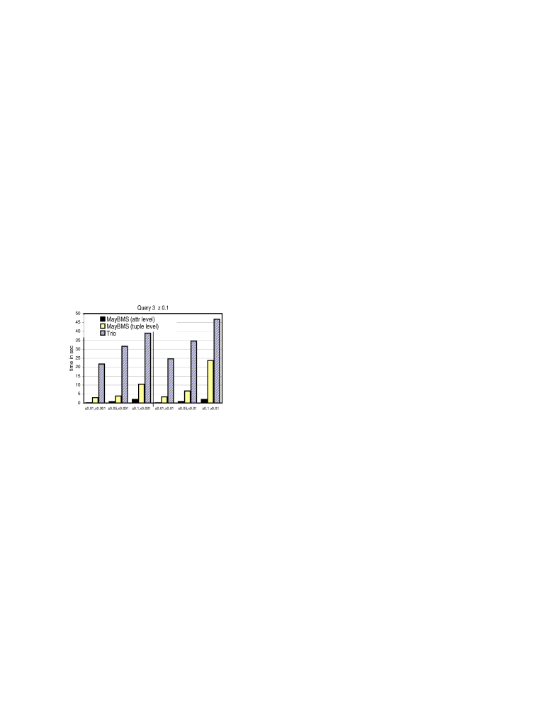
Figure 14: Querying attribute- and tuple-level U-relations in MayBMS and ULDBs in Trio.

Figure 14 compares the evaluation time on attribute- and tuple-level U-relations in MayBMS, and ULDBs for small scenarios of 1% uncertainty, our lowest correlation factor 0.1, and scale up to 0.1. On attribute-level U-relations, the queries perform several times better than on tuple-level U-relations and by an order of magnitude better than ULDBs. This is because attribute-level data allows for late materialization: selections and joins can be performed locally and tuple reconstruction is done only for successful tuples. We witnessed that an increase in any of our parameters would create prohibitively large (exponential in the arity) tuple-level representations. For example, for scale 0.01 and uncertainty 10%, relation lineitem contains more than 15M tuples compared to 80K in each of its vertical partitions.

7 Conclusion and Future Work

This paper introduces U-relational databases, a simple representation system for uncertain data that combines the advantages of existing systems, like ULDBs and WSDs, without sharing their drawbacks. U-relations are exponentially more succinct than both WSDs and ULDBs. Positive relational algebra queries are evaluated purely relationally on U-relations, a property not shared by any other previous succinct representation system. Also, U-relations are a simple formalism which poses a small burden on implementors.

We next briefly report on two current research directions.

Probabilistic U-relations. U-relational databases can be elegantly extended to model probabilistic information by just adding a probability column $P$ to the world table $W$. For each variable $x$, the sum of the values $\pi_{P}(\sigma_{\mathrm{Var}=x})(W)$ must equal one. We can then assign probability to any subset of the world-set, described by a ws-descriptor $\overline{d}$, as the product of probabilities of each variable assignment in $\overline{d}$.

The techniques for evaluating the operations of positive relational algebra presented in this paper are applicable in the probabilistic case without changes. Computing the confidences of the answer tuples is an inherently hard problem [10]. Our current research investigates practical approximation techniques for confidence computation.

Support for new language constructs. Following our recent investigation on uncertainty-aware language constructs beyond relational algebra [5], we identified common physical operators needed to implement many primitives for the creation and grouping of worlds. It appears that normalizing sets of ws-descriptors in the sense of Section 4 plays an important role in evaluating these operations and in confidence computation. We are currently working on secondary-storage algorithms for normalization.

References

- [1] S. Abiteboul, P. Kanellakis, and G. Grahne. “On the representation and querying of sets of possible worlds”. Theor. Comput. Sci., 78(1), 1991.
- [2] P. Andritsos, A. Fuxman, and R. J. Miller. “Clean Answers over Dirty Databases: A Probabilistic Approach”. In Proc. ICDE, 2006.
- [3] L. Antova, T. Jansen, C. Koch, and D. Olteanu. “Fast and Simple Relational Processing of Uncertain Data”. Technical Report INFOSYS-TR-2007-2, Saarland University, 2007.
- [4] L. Antova, C. Koch, and D. Olteanu. “ Worlds and Beyond: Efficient Representation and Processing of Incomplete Information”. In Proc. ICDE, 2007.
- [5] L. Antova, C. Koch, and D. Olteanu. “From Complete to Incomplete Information and Back”. In Proc. SIGMOD, 2007.
- [6] L. Antova, C. Koch, and D. Olteanu. “World-set Decompositions: Expressiveness and Efficient Algorithms”. In Proc. ICDT, 2007.
- [7] D. S. Batory. “On Searching Transposed Files”. ACM Trans. Database Syst., 4(4):531–544, 1979.
- [8] O. Benjelloun, A. D. Sarma, A. Halevy, and J. Widom. “ULDBs: Databases with Uncertainty and Lineage”. In Proc. VLDB, 2006.
- [9] R. Cheng, S. Singh, and S. Prabhakar. “U-DBMS: a database system for managing constantly-evolving data”. In Proc. VLDB, 2005.
- [10] N. Dalvi and D. Suciu. “Efficient query evaluation on probabilistic databases”. In Proc. VLDB, 2004.
- [11] G. Grahne. “Dependency Satisfaction in Databases with Incomplete Information”. In Proc. VLDB, 1984.
- [12] T. Imielinski and W. Lipski. “Incomplete information in relational databases”. Journal of ACM, 31(4), 1984.
- [13] T. Imielinski, S. Naqvi, and K. Vadaparty. “Incomplete objects — a data model for design and planning applications”. In Proc. SIGMOD, 1991.
- [14] P. Sen and A. Deshpande. “Representing and Querying Correlated Tuples in Probabilistic Databases”. In Proc. ICDE, 2007.
- [15] M. Stonebraker, D. J. Abadi, A. Batkin, X. Chen, M. Cherniack, M. Ferreira, E. Lau, A. Lin, S. Madden, E. J. O’Neil, P. E. O’Neil, A. Rasin, N. Tran, and S. B. Zdonik. “C-Store: A Column-oriented DBMS”. In Proc. VLDB, 2005.
- [16] Transaction Processing Performance Council. TPC Benchmark H (Decision Support), revision 2.6.0 edition, 2006. http://www.tpc.org/tpch/spec/tpch2.6.0.pdf.