Trapping of Neutral Rubidium with a Macroscopic Three-Phase Electric Trap

Abstract

We trap neutral ground-state rubidium atoms in a macroscopic trap based on purely electric fields. For this, three electrostatic field configurations are alternated in a periodic manner. The rubidium is precooled in a magneto-optical trap, transferred into a magnetic trap and then translated into the electric trap. The electric trap consists of six rod-shaped electrodes in cubic arrangement, giving ample optical access. Up to $10^{5}$ atoms have been trapped with an initial temperature of around 20 microkelvin in the three-phase electric trap. The observations are in good agreement with detailed numerical simulations.

Trapping is essential in many modern experiments in physics. A trap allows the interaction time of the trapped species with other particles or fields to be greatly extended. Trapping enabled breakthrough experiments with ions, atoms and molecules. Each newly demonstrated trap paved the way for new classes of experiments. Thus far, electric traps for neutral polarizable particles have received relatively little attention. They have first been proposed for excited (Rydberg) atoms WingPRL80 and, later, for ground-state atoms Shimizu92 ; Morinaga94 . Ground-state particles lower their energy in electric fields. Hence these particles are attracted by high fields (“high-field seekers”). Since Maxwell’s equations don’t allow the creation of an electrostatic maximum in free space, time-dependent (pseudo-electrostatic or “AC”) fields are required for trapping, a principle well known from ion traps. Only recently, two-dimensional Junglen04 and three-dimensional Veldhoven05 versions of AC traps have been demonstrated with cold polar molecules having a large and linear Stark shift. For polar molecules, these traps offer the advantage of a deep trapping potential, which can trap both low- and high-field seeking states. Using laser-cooled strontium atoms, the Katori group has demonstrated a chip version of an AC electric trap with the motivation of performing precision spectroscopy for metrology Kishimoto06 .

In this Letter we report on an experiment where laser-cooled rubidium atoms are trapped in a macroscopic AC electric trap. This result opens the perspective of confining cold molecules and atoms in the same spatial region for the purpose of using the optically cooled atoms as a coolant for the molecules. For this, a large volume of several mm³, ample optical access and a relatively deep effective potential depth are essential. The geometry of our trap is in essence the one proposed in Shimizu92 ; Morinaga94 with rectangular driving. Our trap is a three-phase trap, i.e., a full cycle of its operation can be divided in three different phases. The three-phase trap offers cubic symmetry rather than the cylindrical one of three-dimensional two-phase traps Peik99 . Therefore, the average restoring force is isotropic about the trap center Wuerker59 .

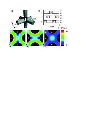
Figure 1: (color online) The AC electric trap. a) the 6 electrodes. b) the switching diagram, indicating that in each full cycle each pair of electrodes is switched on for one third of the time. c)-e) the absolute value of the electric field in the $x-y$ plane in the three consecutive phases of a full driving cycle with electrodes at $\pm 7\,$kV.

Our trap is depicted in Fig. 1. It consists of three pairs of electrodes in a cubic arrangement. Trapping is achieved by alternating the electric field configuration in a cyclic manner with driving frequency $f$. The phase of the driving field is $\phi=2\pi t/T\mod 2\pi$, with $t$ the time and $T=1/f$ the period. At each point of time, only two opposing electrodes are given large voltages of opposite sign; the other four electrodes are grounded. This leads to an electric field of which the absolute value $|E|$ has the shape of a saddle, increasing towards the two charged electrodes and decreasing in the two perpendicular directions. In the following we first focus on the field near the trap center. Assuming that in the first phase of the driving cycle the electrodes in the x direction are charged, the electric field strength can here be approximated in second order in the spatial coordinates by

$$|E|=E_{0}+bx^{2}-\frac{1}{2}b(y^{2}+z^{2})\ \ 0\leq\phi<2\pi/3,$$ (1)

where in our experiment $E_{0}=30.4\,$kV/cm and $b=19.8\$ kV/cm/mm² are coefficients found from the full numerical field calculation Simion with the $x$ electrodes at $\pm 7\,$kV. Atoms experience a quadratic Stark shift in this field: $W_{\rm S}=-\frac{1}{2}\alpha|E|^{2}$, where $\alpha$ is the atom’s static polarizability RbPolarizability . Due to the gradients in $|E|$, the field exerts a force ${\mathbf{F}}=-\nabla W_{\rm S}$ on the atoms. This force pushes the atoms towards the high electric fields near the surfaces of the charged electrodes. This defocusses the atom cloud in the $x$ direction during $0\leq\phi<2\pi/3$. At the same time, the atoms are focussed in the $y$ and $z$ direction. In the second phase of the trap cycle ($2\pi/3\leq\phi<4\pi/3$), the pair of electrodes in the $y$ direction is charged while simultaneously the $x$ and $z$ pair are grounded. Now the $y$ direction is defocussing, whereas the $x$ and $z$ direction are focussing. In the third and last phase ($4\pi/3\leq\phi<6\pi/3$), the focussing and defocussing directions are permutated once more. With the additional approximation that ${\mathbf{F}}=\alpha|E|\nabla|E|\approx\alpha E_{0}\nabla|E|$, the force on an atom at a given point in space averages to zero in a full cycle. However, under the influence of the periodic driving the atom moves and the average force over a full cycle is finite and directed to the trap center. Assuming the drive frequency is high enough, the motion can be be divided in two parts: the cyclic motion locked to the driving field is called the micromotion; the motion under influence of the average force is called the secular motion. For large drive frequencies one can average over the micromotion to find the average restoring force yielding the secular motion. For a driving frequency below a certain cut-off value, the micromotion becomes unstable, the atoms hit the electrodes and are lost.

The equations of motion derived from ${\mathbf{F}}\approx\alpha E_{0}\nabla|E|$ with $|E|$ from Eq. (1) can be solved analytically Shimizu92 ; Morinaga94 . From a stability analysis, analytic expressions for the cut-off frequency are found. For atoms, which have a quadratic Stark shift, the cut-off frequency is linear in the applied voltage. For high $f$, the trap depth decreases with $1/f^{2}$, so the maximum depth is obtained for frequencies just above the cut off, and its position, $f_{\rm peak}$, is also expected to scale linear in the applied voltage.

From previous studies Junglen04 we know that the regions away from the center, where there are no known analytic solutions of the equations of motion, play an important role. Therefore, extensive Monte Carlo simulations were performed to study the performance of the trap in detail. In these simulations, the Newtonian equations of motion are solved for typically $10^{4}$ particles for a single parameter setting. All parameters in the simulation are fixed by the experiment. For the electric field in the simulation, the exact three-dimensional calculation was used Simion .

Our experimental realization of the trap has titanium electrodes mounted on a claw-like ceramic mount. The diameter of the electrode rods is 3 mm, which is also the distance between opposing electrodes. The radius of curvature of the half-spherical endings is 1.5 mm. The electrodes can be charged to $\pm 7\,$kV in a time shorter than a microsecond. The (four) diagonals through the trap offer free sight with a diameter of 1.9 mm. The trap is oriented such as to allow for three optional orthogonal optical paths parallel and perpendicular to the horizontal plane. Along these three axes, the free view is 1.4 mm. Due to the tilted mounting, gravity is pointing in the $(-0.67,-0.67,-0.33)$ direction of the cartesian coordinate system coinciding with the axes of the electrodes.

The electric trap is loaded with laser-cooled ⁸⁵Rb atoms. The atoms are captured from a dispenser in a MOT placed at a horizontal distance of 2 cm from the center of the electric trap. As measured by absorption imaging, $2\times 10^{7}$ atoms are captured here. Before transferring the atoms to a magnetic trap, they are cooled by optical molasses molasses to a temperature of $\approx 15\,\mu$K in 7 ms and optically pumped to the $F=3,m_{F}=3$ Zeeman state. The magnetic trap is generated by two water-cooled coils with 48 windings which are rated to hold 75 A for 3 seconds. The coils are mounted on a translation stage. By moving the coils, the magnetic field minimum and the atoms are translated Lewandowski03 . After bringing the atoms in approximately $0.8\,$s into the center of the electric trap, the magnetic trap is switched off in $25\,\mu$s and the electric trap is switched on $100\,\mu$s later. To determine the initial conditions of the atoms before the start of the electric trap, we kept the atoms at the position of the MOT and measured the cloud to contain $6\times 10^{6}$ atoms and to have a temperature of $62\,\mu$K. In a separate experiment, it was tested that moving the magnetic trap causes no significant heating or losses.

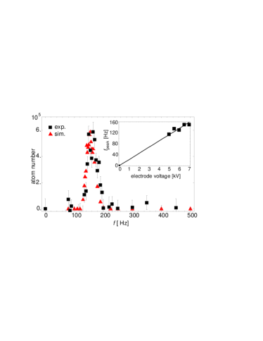
Figure 2: (color online) The frequency dependence of the trapped number of atoms after 50 ms for electrodes at $\pm 7\,$kV. The square symbols are data, the triangles are the result of a Monte Carlo simulation. Noise in the background images can lead to negative values. The simulation result is scaled to fit the height of the data. The inset shows the measured dependence of the frequency of the maximum $f_{\rm peak}$ as a function of the electrode voltage. The expected linear dependence is indicated by the line.

A number of different measurements was performed to characterize the electric trap: the dependence of the number of trapped atoms on time, drive frequency and electrode voltage was studied and is discussed in the following. The number of particles remaining in the electric trap after 50 ms was measured by absorption imaging. The results are depicted in Fig. 2 as a function of the drive frequency. There is a sharp cut off near 120 Hz. Just above the cut off, the maximum number of atoms is trapped. As expected, the frequency of the maximum, $f_{\rm peak}$, scales linearly in the applied voltage (see the insert of Fig. 2). In the limit of high frequencies, the micromotion becomes smaller and faster and the net force towards the trap center vanishes. Therefore, the trap depth, and hence the number of particles, falls off quickly with $f$. The simulation describes the position and the shape of the trapping peak very well. The absolute fraction of trapped atoms is very sensitive to temperature, size and position of the initial atomic cloud. Nevertheless, this fraction obtained from the simulation agrees with the measurement within a factor of two. For trapping times below 50 ms, the atom number as a function of driving frequency shows more complex structures (not shown), both in the simulation and in the experiment, which is attributed to atoms which are released from the magnetic trap into unstable orbits of the electric trap.

The number of remaining atoms as a function of time is plotted in Fig. 3. The atoms escaping the trap from unstable orbits causes the loss which is observed for times shorter than 50 ms. The simulation predicts this rapid initial loss. It also predicts stable trapping after $50-80\,$ms. The observed signal, however, falls off with a time constant of $0.36\,$s. The pressure in the UHV chamber is in the $10^{-10}\,$mbar range during MOT operation, which is too good to explain this loss. However, during operation of the electric trap, significant pressure rises are observed by a remote pressure gauge. Also the lifetime in the magnetic trap just outside the electrodes is observed to go down from almost 2 s to the few 100 ms regime when high voltage is applied. From this and other observations we deduce that gas, probably Rb absorbed on the electrodes, is ejected from the electrodes once they are charged up, locally increasing the pressure and limiting the lifetime of trapped atoms. Therefore, we are confident that the observed decay is due to collisions with hot background atoms released from the electrodes.

The maximum number of trapped atoms depends not only on the drive frequency and time but also on the applied voltages. In the inset in Fig. 3, the number of atoms in the maximum is plotted as a function of the applied voltages. Again, the simulation describes the results well. Below 4 kV, trapping is no longer possible due to the gravitational force exceeding the cycle-averaged electric trapping force.

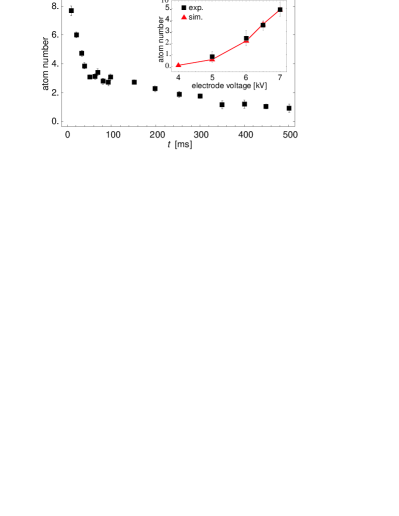
Figure 3: (color online) Remaining number of atoms as a function of time. At $t=0$ the magnetic trap contains $2.7\times 10^{6}$ atoms. The initial rapid decay is caused by atoms which enter the electric trap on non-trapped orbits, either because they are too hot or because their motion has the wrong phase. The decay of the trapped atoms, visible as the long tail with a $1/e$ time of 0.36 s, is attributed to collisions with back-ground gas. The inset shows, for another set of data with other starting conditions, the dependence of the maximum number of trapped atoms after 50 ms electric trapping as a function of the applied voltage. The line is a guide to the eye.

Absorption imaging of the trapped cloud allows additional insight into its dynamics. Images spanning more than a full cycle of the AC trap are depicted in Fig. 4. The atom cloud is ellipsoidal, but the ellipticity varies periodically in time. This is caused by the periodic motion of the individual atoms, making the cloud pulsate. To demonstrate the correspondence between the simulation and the measurements, we calculate the ellipticity of the measured and simulated clouds by projection onto their two major axes. From this the aspect ratio is calculated and plotted in Fig. 4c). The agreement is very good; the remaining differences are attributed to imaging imperfections. Note the difference in the minimum ellipticity at 50.5 and 56 ms, which is predicted by the simulation and caused by a residual vertical oscillation of the cloud under influence of gravity with a longer periodicity.

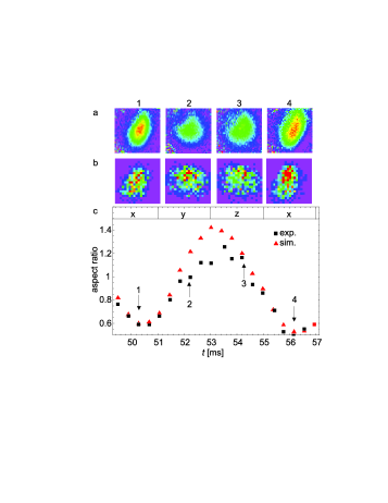
Figure 4: (color online) a) Measured and b) simulated camera pictures of the trapped cloud at the times indicated $1,2,3,4$ in c). Each picture in a) is an average over 10 measurements. The $19.5^{\circ}$ tilt with respect to the vertical corresponds to the tilt angle of the trap mounting. c) Measured (squares) and simulated (triangles) aspect ratio of the elliptic clouds. The boxes with letters $x,y,z,x$ indicate the charged electrodes. Note that the simulation has no free parameters.

As a final characterization of the trap, its depth and the temperature of the trapped cloud should be discussed. From expansion data, temperatures of the trapped cloud can be obtained. However, the expansion of the cloud is dominated by the velocities of the micromotion, which remain constant in the falling frame of reference when the electric fields are switched off. The ellipticity observed in Fig. 4 already indicates that the expansion will be anisotropic. Indeed, different temperatures are measured depending on the phase when the trap is switched off. At a driving frequency of 170 Hz and release from the electric trap after 21 ms, temperatures of $63\,\mu$K and $122\,\mu$K were measured in two orthogonal directions. One could argue, however, that these numbers are not good measures for the trap depth. More relevant is the depth of the effective potential, which in the harmonic limit is obtained by averaging over the micromotion. Here the simulation is again of help: it allows to extract the initial velocity distribution of those atoms which remain trapped in stable orbits. For a cloud of an initial size of 0.3 mm, this distribution corresponds to $20\,\mu$K. We use this number as a definition of the effective trap depth.

There are two natural ways to improve the system. The lifetime could be extended by improving the background pressure during operation of the electric trap. The MOT could be placed further away from the electric trap or even in a separate, differentially pumped, chamber. A second improvement concerns gravity. The simulations show that without gravity, the trap depth is approximately doubled. This implies that significantly more particles could be trapped by compensating for gravity. This can, in principle, be achieved by applying asymmetric voltages on the electrodes, shifting the saddle point of the electric field up, causing a net electric force to outbalance gravity. This is more straightforward when the trap is rotated such that one of the electrode pairs is oriented vertically.

In principle, simultaneous trapping of atoms and molecules in our trap is possible, enabling ultracold collision studies once sufficiently high densities and sufficiently long trapping times are achieved. Simultaneous trapping should work for molecules like H₂O or D₂O which have, firstly, a quadratic Stark shift RiegerPRA06 and, secondly, several thermally populated states with a similar polarizability over mass ratio as ⁸⁵Rb. Other alkalis and higher-order stability islands could also be exploited. Another possibility is to overlay a magnetostatic trap for atoms with a tens of mK deep electrodynamic trap for molecules with a large Stark shift. Since optimal switching frequencies for such molecules are in the kHz range Junglen04 ; Veldhoven05 , these fields will only make a very weak potential for the atoms. Hence, sympathetic cooling of cold molecules by laser-cooled atoms might be possible. Other applications of our setup are trapping of atoms or molecules in Rydberg states and the study of atom-atom interaction at ultralow temperatures by electric fields Marinescu98 or combined electric and magnetic fields Krems05 .

During the final preparation stages of this manuscript, similar results were reported elsewhere Schlunk07 .

We thank S. Nußmann for help with the experiment. We acknowledge financial support by the Deutsche Forschungsgemeinschaft (SPP 1116, cluster of excellence Munich Centre for Advanced Photonics).

References

- (1) W.H. Wing, Phys. Rev. Lett. 45, 631 (1980).
- (2) F. Shimizu and M. Morinaga, Jpn. J. Appl. Phys. 31, L1721 (1992).
- (3) M. Morinaga and F. Shimizu, Las. Phys. 4, 412 (1994).
- (4) T. Junglen, T. Rieger, S.A. Rangwala, P.W.H. Pinkse, and G. Rempe, Phys. Rev. Lett. 92, 223001 (2004).
- (5) J. van Veldhoven, H.L. Bethlem, and G. Meijer, Phys. Rev. Lett. 94, 083001 (2005); H.L. Bethlem, J. van Veldhoven, M. Schnell, and G. Meijer, Phys. Rev. A 74, 063403 (2006).
- (6) T. Kishimoto, H. Hachisu, J. Fujiki, K. Nagato, M. Yasuda, and H. Katori, Phys. Rev. Lett. 96, 123001 (2006).
- (7) E. Peik, Eur. Phys. J. D 6, 179 (1999).
- (8) R.F. Wuerker, H.M. Goldenberg, and R.V. Langmuir, J. Appl. Phys. 30, 441 (1959).
- (9) Calculated with the software package “Simion”.
- (10) For Rb, kHz/(kV/cm)2; CRC Handbook of Chemistry, CRC Press, 85th edition, 2004-2005.
- (11) P.D. Lett, W.D. Phillips, S.L. Rolston, C.E. Tanner, R.N. Watts, and C.I. Westbrook, J. Opt. Soc. Am. B 6, (1989).
- (12) H.J. Lewandowski, D.M. Harber, D.L. Whitaker, and E.A. Cornell, J. Low Temp. Phys. 132, 309 (2003).
- (13) T. Rieger, T. Junglen, S.A. Rangwala, G. Rempe, P.W.H. Pinkse, and J. Bulthuis, Phys. Rev. A 73, 061402(R) (2006).
- (14) M. Marinescu and L. You, Phys. Rev. Lett. 81, 4596 (1998).
- (15) R. Krems, Int. Rev. Phys. Chem. 24, 99 (2005); B. Marcelis, B.J. Verhaar, and S.J.J.M.F. Kokkelmans, private communication.
- (16) S. Schlunk, A. Marian, P. Geng, A.P. Mosk, G. Meijer, and W. Schöllkopf, Phys. Rev. Lett. 98, 223002 (2007).